HAL Id: hal-00008701
https://hal.archives-ouvertes.fr/hal-00008701
Preprint submitted on 15 Sep 2005
HAL is a multi-disciplinary open access
archive for the deposit and dissemination of
sci-entific research documents, whether they are
pub-lished or not. The documents may come from
teaching and research institutions in France or
abroad, or from public or private research centers.
L’archive ouverte pluridisciplinaire HAL, est
destinée au dépôt et à la diffusion de documents
scientifiques de niveau recherche, publiés ou non,
émanant des établissements d’enseignement et de
recherche français ou étrangers, des laboratoires
publics ou privés.
Robust Routing and Cross-Entropy Estimation
Hélène Le Cadre
To cite this version:
ccsd-00008701, version 1 - 15 Sep 2005
ROBUST ROUTING AND
CROSS-ENTROPY ESTIMATION
H´el`ene Le Cadre
[email protected]
ENST, Bretagne
September 9, 2005
1
Introduction
In this article we present a novel way to estimate the amounts of traffic on the Origin-Destination couples (OD couples). This new approach combines together a routing algorithm based on the principle of the shortest path and a recent technique of stochas-tic optimization called Cross-Entropy. The CE method was built at the origin, to tackle problems of raevent simulation. However, its inventor, R. Rubinstein, re-alized soon that the underlying idea should be applied efficiently to combinatorial and multi-extremal optimization problems.
In a final part, we adapt a particular filtering algorithm in order to be able to dynami-cally estimate the evolution of the traffic on the OD couples.
The aim of this report is to highlight rather original ideas, however the choices of the prior distributions and some specific parameters may be quite arbitrary.
2
A brief presentation of the CE method
2.1
Rare-Event Simulation
Let X = (X1, ..., XN), be a random vector taking values in a space called X . Let
{f (.; v)} be a family of parametric densities defined on the space X , with respect to
the Lebesgue measure. For any measurable function H, we can define:
E[H(X)] = Z
Ξ
H(x) f (x; v) dx .
The performance function will be called S : X → R. For a fixed level γ, we are
interessed in the probabilty of the event defined below:
If this probability is very small, for example not more than10−5, the set{S(x) ≥
γ} will be called a rare event.
A straightforward way to estimate l may be to use crude Monte-Carlo simulation: let
(X1, ..., XN) be a sample drawn from the density f (.; u). Then, the estimator,
1 N N X i=1 1{S(x) ≥ γ}
is an unbiased estimator of l. However, if {S(x) ≥ γ} is a rare event, many
indicator functions will remain equal to zero. As a result, we will be forced to simulate huge samples, which is rather costly and difficult to put in application.
Another way to get an estimate of l might be to use importance sampling. We should draw(X1, ..., XN) from a density g , defined on the space X . This density is nothing
else than a mere change of measure. The estimator then becomes:
ˆ l = 1 N N X i=1 1{S(Xi) ≥ γ} f(Xi; u) g(Xi) . (1) The optimal density g, is defined by:
g⋆(x) = 1{S(x) ≥ γ} f(x; u) l . (2) Substituting(2) in (1), we get: 1{S(Xi) ≥ γ} f(Xi; u) g⋆(X i) = l , ∀ i .
But, l is a constant. As a result, the estimator defined in(1) has zero variance.
Nev-ertheless, g⋆depends on the unknown parameter l. The idea is in fact, to choose g in a parametric family of densities{f (.; v)}. The problem is now to determine the optimal
parameter v, such that the distance between g⋆and f(.; v) should be minimized.
A well-known ”distance” between two densities g and h, is the Kullback-Leibler ”dis-tance”: D(g, h) = Eg[ln g(X) h(X)] = Z g(x) ln g(x) dx − Z g(x) ln h(x) dx . (3) Minimizing the Kullback-Leibler distance between g⋆and f(.; v), is equivalent to
solve the following problem:
arg max v Z g⋆(x) ln f (x; v) dx . (4) Substituting(2) in (4), we get: arg max v D(v) = arg maxv Eu[1{S(X) ≤ γ}ln f(X; v)] . (5)
But, in fact we can estimate v⋆, by solving the following stochastic program: arg max v ˆ D(v) = arg max v 1 N N X i=1 [1{S(Xi) ≥ γ}ln f(Xi; v)] . (6)
If ˆD is convex and differentiable in v, we just have to solve the following problem: 1 N N X i=1 [1{S(Xi) ≥ γ}∇vln f(Xi; v)] = 0 . (7)
The solution can often be calculated analytically, which is one of the great advan-tages of this approach.
2.2
Application of the CE to optimization
Usually, in the field of optimization we try to solve problems of the form:
S(x⋆) = γ⋆ = arg max
x∈X S(x) . (8)
The genius of the Cross-Entropy method lies in the fact that it is possible to asso-ciate with each optimization problem of the form(8), a problem of estimation, called associated stochastic problem (ASP). We will start by defining a collection of indicator
functions{1{S(x) ≤ γ}}γ∈ R, on the spaceX . Then, we will define a parametric
fam-ily of densities{f (.; v), v ∈ V} on the space X . Let u ∈ V. We will associate with (8), the following stochastic estimation problem:
l(γ) = Pu(S(X) ≥ γ) =
X
x
1{S(x) ≥ γ} f(x; u) = Eu[1{S(x) ≥ γ}] , (9)
If γ = γ⋆, a natural estimator of the reference parameter v⋆is:
ˆ v⋆ = arg max v 1 N N X i=1 1{S(x) ≥ γ}ln f(Xi; v) , (10)
where the Xi are drawn from the density f(., u). If γ is very close to γ⋆, then
f(.; v⋆) assigns most of its probability mass close to x⋆. In fact, in this case, we will
have to choose u so thatPu(S(X) ≥ γ) is not too small. We can infer that u and γ
are closely linked.
We will use a two level procedure. Indeed, we will construct two sequencesγˆ1, ...,γˆT
andvˆ0,vˆ1, ...,vˆT such thatγˆT is close to γ⋆ andvˆT is such that the density assigns
most of its mass in the state which maximizes the performance. The algorithm follows a two-step strategy:
• Generate a sample (X1, ..., XN) ∼ f (.; vt−1). Compute the (1 − ρ)-quantile
of the performance S, which can be estimated by: ˆ
γt = S[(1−ρ)N ].
• Use the same sample (X1, ..., XN), to solve (6). Call the solution vt.
• If for some t ≥ d, d fixed, ˆ
γt= ... = ˆγt−d,
Stop; otherwise set t= t + 1 and reiterate from Step 2.
3
The Model
The network we study is composed of p nodes and n arcs. At first, we will suppose that there exists an arc between each couple of nodes. Furthermore, we make the difference between the two couples(i, j) and (j, i), ∀ i, j ∈ {1, ..., n}, i 6= j.. Consequently,
n = p2 − p .
Recall that an arc is a directed link. In the rest of this article, we will make the hypoth-esis that the network is directed.
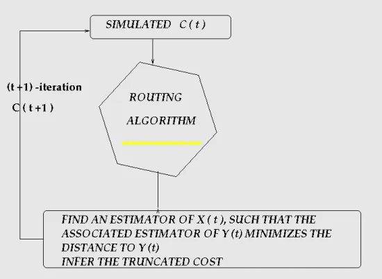
Our work could be separated into two different parts. Firstly, we have to deal with a simulation part. In this section, we will choose an initial vector of the amounts of traffic on the OD couples. Our aim will be to minimize the global sum of the costs, which are associated to each arc of the network. Secondly, we will have to cope with an estimation part. Indeed, we will suppose that the initial costs are equal to those obtained by the simulation part. The idea then, will be to find the estimator ˆX(t) from
which we could infer an arc estimator ˆY(t) minimizing the distance to the vector Y (t),
obtained in the simulation part. This raises the crucial question of the identifiability of the vector X(t). Is there unicity of the associated vector ˆX(t) or, is it only an element
in a vast variety?
3.1
Simulation
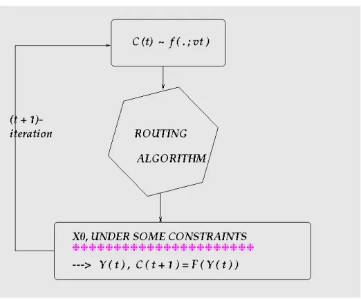
In this part, we associate a cost function to the network, which means that we give a cost to each arc of the network. This cost function is drawn from a parametric families of densities. Which means that we have to determine the optimal parameter of the density function. What’s more, this cost may or, may not be, proportionnal to the amount of traffic on each arc. However, it is more unconventional to suppose that the costs depend on the arc traffic. Let Y(t) be the vector which contains the amount of traffic on each
arc of the network and C(t) the vector which represents the costs associated with each
arc. In the most general case, we have:
C(t) = F (Y (t)) , (11) where F is supposed to be continuous and differentiable.
Figure 1: Simulation.
Then, using these costs, we will use a routing algorithm based on the principle of the shortest path in order to find the shortest paths between each OD couple. A path is represented by the nodes or the arcs which it is made of.
The principle of the routing algorithm we use is rather simple. The first observation to make is that every subpath of a shortest path is necessarily itself a shortest path.
Let ei,jbe the arc linking the nodes i and j. If the path composed of the arcs{ei,j, ej,k, ek,l, ..., ep,q}
is the shortest path linking node i to node q. Then, ei,j must be the shortest path
be-tween i and j. ej,kmust be the shortest path between j and k, and so on...
shortest path must be composed exclusively of basic arcs. The aim of our routing algo-rithm is to substitute to each arc which is not basic, a basic arc. Let di,j = C(t; i, j)
be the distance or weight associated to the arc{i, j}, at the instant t. Let j be the indice
of a node of the network, then:
∀ i , k ∈ Network − {j} , di,k ← min{di,k, di,j+ dj,k} .
The algorithm tests all the couple of nodes(i, k), which are neighbors of j, while j takes each node of the network as its own value.
Algorithm 2. Input: C(t), vector of the costs. • If di,k ≥ di,j+ dj,k, do not change anything.
• If di,k ≤ di,j + dj,k, create an arc linking i to k and associate the weight
di,k = di,j+ dj,k.
Output: the shortest paths between each OD couple.
The algorithm also gives us the shortest distances associated to each OD couple. But, these distances are only rought estimators of the amounts of traffic on each OD couple. Indeed, more than one link, can be shared by different shortest paths linking different OD couples. As a result, the total amount of traffic generated by one OD couple usually represents only a fraction of the total traffic flowing through the arcs which composed the path.
In order to solve this crucial problem, we will associate to the vector which contains the volumes of traffic on the OD couples, called X0(t), an estimator of the volumes of
traffic flowing through the arcs, which we will note Y(t). Indeed, if we use the routing
algorithm, it is quite easy to deduce Y(t) from X0(t). Our goal will be to solve the
following optimization problem:
min n X i=1 |Ci(t)| . (12)
3.2
Estimation
In this part, the performance function is defined by:
S(X(t)) = arg max ˆ X(t) 1 kY (t) − ˆY(t)k2 . (13)
Figure 2: Connection between OD couples and arcs.
The first observation is that S is an implicit function of X(t), e.g. we can’t get any
exact analytical expression of S. Consequently, we will have to resort to use simulation. What’s more, we suppose that the vector X(t) is generated from an exponential
density whose parameter is totally unknown.
X(t) ∼ E(λ), λ ∈ Rn
+ . (14)
We apply the Cross-Entropy method to our problem. At each iteration, we generate a random sample(X(1), ..., X(N )) ∼ E(λ), λ ∈ Rn
+.
Hypothesis: Each component of X(t), which represents the amount of traffic on
an OD couple, will be supposed to be independent of the others.
Practically, each random vector from the sample will be stocked in a big matrix.
X(t) = X1(1) · · · X1(N ) X2(1) · · · X2(N ) .. . ... ... Xn(1) · · · Xn(N ) . (15)
Figure 3: Estimation
The joined densities of the vectors X(j), j= 1, ..., N , are typically of the form: f(X(j), λ) = n Y i=1 λi exp[−λiXi(j)] 1R+(Xi(j)) , = n Y i=1 λi exp[−λiX (j) i ] 1{min(Xi(j)) ≥ 0}. (16)
As a result, we will have to solve the following problem:
1 N N X i=1 1{S(X(i)) ≥ ˆγ t}∇λln f(X (i); λ) = 0 . (17)
After some computations, we get:
λj = PN i=11{S(X(i)) ≥ ˆγ t} [PN i=11{S(X(i)) ≥ ˆγ t}X (i) j ] , ∀ j = 1, ..., n . (18) Remark.
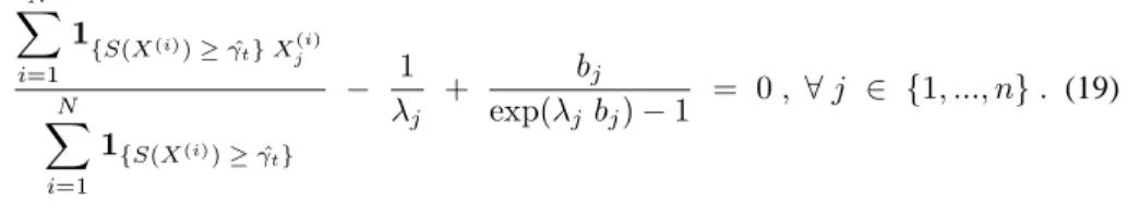
If we generate the random vectors Xi, i= 1, ..., N from a truncated exponential, we
Recall that a truncated exponential is of the form:
f(x; λ, b) = λ exp[−λ x]
1 − exp(−λ b) 1[0,b](x) .
Under this assumption, we have to cope with the following system:
N X i=1 1{S(X(i)) ≥ ˆγ t} X (i) j N X i=1 1{S(X(i)) ≥ ˆγ t} − 1 λj + bj exp(λj bj) − 1 = 0 , ∀ j ∈ {1, ..., n} . (19)
This system is non-linear, that’s why we use the well-known iterative Newton’s method to solve it.
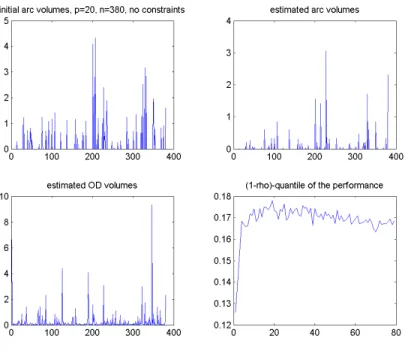
Figure 5: Simulation,20 nodes network, 380 arcs.
4
The problem of Identifiability
We observe that the amount of traffic which flows through each arc of the network is equal to the sum of the amounts of traffic flowing on each OD couple which owns this arc in its shortest path. Remember that, thanks to the routing algorithm, we associate to each OD couple, a unique shortest path. Mathematically, we can express this remark under the following expression:
n
X
j=1
1{ei∈ OD couple number j’s path(t)}Xj(t) = Yi(t) , ∀ i ∈ {1, ..., n}. (20)
More generally, we get:
Y(t) = A(X(t)) X(t) . (21) Indeed, in the most general case, the routing matrix A relies on the volumes of traffic flowing through each arc at the instant t. But, these arc volumes rely themselves on the OD volumes, X(t). As a result, the routing matrix A(t), is a function of X(t).
A is uniquely made of binary elements: 0 and 1. More explicitely, A(X(t); i, j) = 1 iff, the arc numbered i belongs to the shortest path associated to the OD couple
What’s more, the routing algorithm do not use every arc. Consequently, many rows of the routing matrix equal zero. The associated components in the arc vector Y(t) are at
the same time, null.
But, if we suppress the zero rows of A(X(t)) and the zero components of Y (t), this
leads us to solve a rectangular system of equations. This system is under-determined, that’s why we can’t guarantee the existence of a unique solution.
We can conclude that there is no identifiability between the arc volumes Y(t), and
the OD volumes X(t), at a given time. Indeed, if we take a fixed X(t), we get a
unique associated Y(t), since the routing algorithm determines a unique shortest path
between each OD couples. Reciprocally, if we take some fixed arc volumes, Y(t), we
can’t guarantee the unicity of the solutions of(21). That’s why, we can’t assert that the
associated X(t) is perfectly unique.
A good idea to tackle this problem, is to suppose that some of the OD couples do not accept any traffic. That is, that they remain equal to zero. The goal is to reduce the number of positive OD couples so as to get a system whose routing matrix A(t), is
square or not too far.
The first approach is to suppose that some pre-determined OD couples are ex-culded.
To begin, we may partition, a little arbitrarily, the set of the OD couples into two parts. In the first one, lie the OD couples which remain always equal to zero. And, in the second part, we will suppose that there is some traffic flowing through these OD couples.
We need to generate a sample Z. The components of Z are independent of each other and generated from a Bernoulli density whose parameter is pre-determined. Then, if Z(i) = 0, the OD couple number i, do not accept any traffic.
The time required to perform this simulation is of about1 minute.
A second point of vue should be to suppose that we know at the beginning that only
K OD couples, K ≥ n, are positive. So, we need to modify our CE algorithm. We
need to introduce a matrix, Z(t):
Z(t) = Z1(1) · · · Z1(N ) Z2(1) · · · Z2(N ) .. . ... ... Zn(1) · · · Zn(N ) . (22)
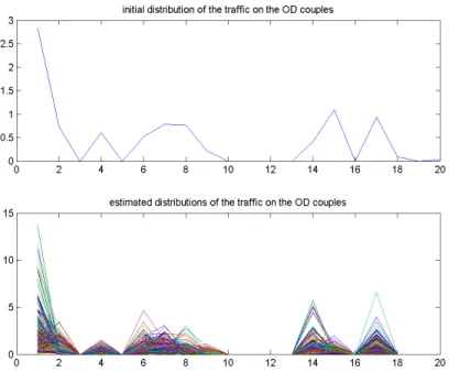
Figure 6: Introduction of constraints on the OD couples: the zero OD couples are pre-determined. Identifiability of X(t) with 23of the OD couples used.
To be more explicit, the ithrow of Z is generated fromB(pi,j(t)), j ∈ {0, 1}, ∀ i ∈
{1, ..., n} . In fact, each row is generated independently from a Bernoulli density
whose parameter is specific, conditional upon the fact thatPn
j=1X (i)
j = K, i ∈
{1, ..., N } . K, is a fixed number. It may be as we have already stated, a certain
prop-portion of OD couples, but it may also take into account some other constraints. The first idea to deal with such a constraint is to generate a random vector X1(i), ..., Xn(i).
Each component are drawn independently from a Bernoulli density. The sample is ac-cepted iff,Pn
j=1X (i)
j = K, i ∈ {1, ..., N } . However, when n becomes higher
than10, it takes a prohibitive time! In fact, the best solution is to generate independant
Bernoulli random variables fromB(p1(t)), B(p2(t)), ..., respectively, until K unities
or n− K zeros are generated. Then, the remaining elements are put equal to zero or
one, respectively. However, the updating formula for the parameters of the Bernoulli densities remain exactly of the form:
pi,1(t) = PN k=1 1{S(X(k)≥ ˆγ t}1{Xi(k)= 1} PN k=1 1{S(X(k)≥ ˆγ t} , ∀ i ∈ {1, ..., n} . (23) In fact, now, X(t) and Z(t) are closely linked. Indeed, if Zi(j) = 0 then, Xi(j) = 0, which means than there is no traffic on the OD couple number i for the jth-sample.
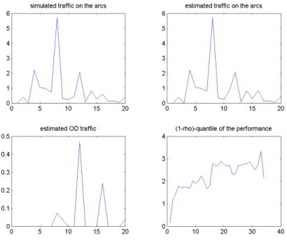
Figure 7: Simulation, the number of zero OD couples is pre-determined, K= 23.
The time required to perform this simulation is of about2 minutes.
5
Dynamic estimation
We have previously determine an estimator of the amounts of traffic flowing through the OD couples at the specific instant t. We should ask ourselves whether it is possible to determine the trajectories associated to the vector X(t). Particle filtering appear to us to be an interesting approach.
5.1
Presentation of Particle filtering
Particle filtering is a well-known technique based on sequential Monte-Carlo approach. It is a technique for implementing a recursive bayesian filter by Monte-Carlo simula-tions. The key ideea is to represent the required posterior density function by a set of random samples with associated weights and to compute estimates based on these
Figure 8: Identifiability of X(t), K =23. samples and weights.
We will generate a random measure{Ci
0:k, wki}i=1,...,M that characterises the
pos-terior pdf p(C0:k | ˆX1:k). {C0:ki , i = 0, ..., M } is a set of vectors with
associ-ated weights {wi
k, i = 1, ..., M } (the weights are themselves vectors of weights).
C0:k = {Cj, j = 0, ..., t} is the set of all states up to time t. The weights are
nor-malised such that,
M
X
i=1
wki,j = 1, ∀ j ∈ {1, ..., n}.
Then, the posterior density at t can be approximated as:
p(C0:k| ˆX1:k) ≈ M
X
i=1
wikδ(C0:k− C0:ki ) . (24)
The weights are chosen using the principle of Importance Sampling. Let Ci ∼
q(.), i = 1, ..., M be samples generated from a proposal q(.), called Importance
sam-pling density. By successive approximations, it is shown in [7] that the weights are
recursively obtained by the following formula:
wik ∝ wk−1i
p( ˆXk|Cki)p(Cki|Ck−1i )
q(Ci
k|Ck−1i , ˆXk)
It can be shown that as M → ∞, the approximation (24) approaches the true
posterior density p(Ck | ˆX1:k).
However, there is a major drawback to use particle filtering techniques. Indeed, a common problem is the degeneracy problem. After a few iterations, all but one particle will have negligable weight. It has been shown that the variance of the importance weights can only increase over time, and thus it is impossible to avoid the degeneracy phenomenon. This degeneracy implies that a large computational effort is devoted to updating particles whose contribution to the approximation to p(Ck| ˆX1:k) is almost
zero.
Consequently, we have to use resampling mechanisms. The basic idea behind resam-pling is to eliminate particles which have small weights and to concentrate on particles with large weights.
5.2
State model and observation equation
The traffic flow will be modelled as a stochastic hybrid system with discrete states. The observation equation is rather simple to get. Indeed, we have:
ˆ
Xk = Ξ(C(k)) . (26)
Where,Ξ is a quite complex function which represent the whole algorithm.
The difficulty now, is to build a state model. Suppose the flow can be decomposed in small entities (for example packets). We note:{Ql′,k|l′ ∈ {arcs of the network}, i →
l′}, the number of packets going out of the arc i, during the time interval [t k, tk+1[.
{Ql,k|l ∈ {arcs of the network}, l → i}, is the number of packets arriving on the arc
i on[tk, tk+1[.
The conservation of the flow lets us write:
Yi(k + 1) = Yi(k) + X {arcs l|l→i} Ql,k − X {arcs l′|i→l′} Ql′,k . (27) In fact,
Qi,k = min(Si,k; Ri,k+1) . (28)
Si,kis called sending function. It expresses how many among the Yi(k) packets in
the arc i at k are at a distance less than a fixed boundary called β. Suppose the interac-tion between the packets is negligible and their locainterac-tion is uniformly distributed over the arc. Si,kis then a random binomial variable with Yi(k) drawings, with probability
of success arc i lengthβ , or an approximation, since we don’t know exactly the length of the arc number i.
The receiving function is defined by: Ri,k+1 = X {arcs l|i→l} [Ymax l (k) + Ql,k+1 − Yl(k)] . (29)
The sending function is calculated at first by forward recursion, and we substitute
Qi,k= Si,kin(27). With this first guess of the amount of traffic in arc i, at time tk+1,
a first guess of the receiving function can be computed, recursively. Finally, we get:
Ci(k + 1) = F (Yi(k + 1)) = Ψ(Yi(k), W (k + 1)) , ∀ i ∈ {1, ..., n}. (30)
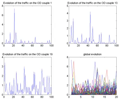
Figure 10: Spatial evolution of the distribution of the traffic at four different instants.
6
Conclusion
We could observe that the performance of the CE method is directly proportionnal to the ratio:
|set of nodes|
|set of OD couples| (31)
For rather small networks, eg. networks composed of at most30 nodes, the CE
method works pretty good and suprisingly fastly. What’s more, it is possible to add some constraints which could guarantee the identifiability of the vector containing the amounts of traffic on the OD couples. At the end of the estimation part, we get estima-tors of OD volumes and implicitly, of the routing matrix. In fact, this application is a great proof of the simplicity and versatility of the CE method.
However, some points remain difficult to tackle. For example, when the ratio becomes
larger than 19, the CE method performs rather poorly. Furthermore, R. Rubinstein
recommand that the sample size of the CE algorithm should be of the form:
N = κ n, 5 ≤ κ ≤ 10 .
Suppose for example, that that we have to deal with a network of50 nodes. Then, at
each step of the algorithm we will have to generate a sample of2450 ∗ 20000 vectors.
Which is completly impossible due to the limited capacities of our computers. But, it is certainly possible to improve the algorithm so as to adapt dynamically the sample size
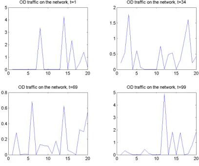
Figure 11: Spatial distribution of the traffic at four instants.
to solve this problem. Nevertheless, the question remains open. Fortunately, in every network, some specific constraints need to be taken into account. These constraints aim at decreasing the number of unknown parameters. The idea to impose that some OD couples remain equal to zero is an approach, but there are many others. For example, we may want to maximize the global entropy, or other common criteria.
Particle Filtering is an efficient and subtle technique to dynamically predict the evolu-tion of the distribuevolu-tion of the traffic on the OD couples for rather small networks. The approaches we use are rather simple to put in application. Nevertheless, they rely on many small parameters which are quite difficult to optimize. Furthermore, the size of the network is still a problem and may be the next challenge of this reflexion.
7
References
[1] RUBINSTEIN Reuven Y., KROESE Dirk P., The Cross-Entropy Method, Springer, 2004.
[2] HU T.C., SHING M.T., Combinatorial Algorithms, Dover Publications, second
edi-tion,2002.
[3] SCHRJVER A., Theory of Linear and Integer Programming, John Wiley, 2000. [4] RARDIN R. L., Optimization in Operations Research, Prentice Hall, 1998. [5] DOUCET A., MASKELL S., GORDON N., Particle Filters for Sequential Bayesian
Inference, Tutorial ISIF,2002.
[6] MIHAYLOVA L., BOEL R., A Particle Filter for Freeway Traffic Estimation. [7] ARULAMPALAM S., MASKELL S., GORDON N., CLAPP T., A Tutorial on
Par-ticle Filters for On-line Non-linear/Non-Gaussian Bayesian Tracking, IEEE,2001.
[8] CAMPILLO F., LE GLAND F., Filtrage Particulaire: quelques exemples ”avec les