HAL Id: hal-01426623
https://hal.archives-ouvertes.fr/hal-01426623
Submitted on 4 Jan 2017
HAL is a multi-disciplinary open access
archive for the deposit and dissemination of
sci-entific research documents, whether they are
pub-lished or not. The documents may come from
teaching and research institutions in France or
abroad, or from public or private research centers.
L’archive ouverte pluridisciplinaire HAL, est
destinée au dépôt et à la diffusion de documents
scientifiques de niveau recherche, publiés ou non,
émanant des établissements d’enseignement et de
recherche français ou étrangers, des laboratoires
publics ou privés.
Study of Dipole Antennas’ Characteristic Modes
Through the Antenna Current Green’s Function and the
Singularity Expansion Method
Francois Sarrazin, Mikki Said, Yahia Antar, Philippe Pouliguen, Ala Sharaiha
To cite this version:
Francois Sarrazin, Mikki Said, Yahia Antar, Philippe Pouliguen, Ala Sharaiha. Study of Dipole
An-tennas’ Characteristic Modes Through the Antenna Current Green’s Function and the Singularity
Expansion Method. European Conference on Antennas and Propagation (EuCAP), Apr 2015,
Lis-bonne, Portugal. �hal-01426623�
Study of Dipole Antennas’ Characteristic Modes
Through the Antenna Current Green’s Function and
the Singularity Expansion Method
Francois Sarrazin
13, Said Mikki
1, Yahia Antar
1, Philippe Pouliguen
2, Ala Sharaiha
31 Royal Military College of Canada, Kingston, Canada, [email protected] 2 Direction Generale de l’Armement, Bagneux, France, [email protected]
3 Institute of Electronics and Telecommunications of Rennes, University of Rennes 1, France, [email protected]
Abstract—This paper deals with modelling the Antenna Current Green’s Function (ACGF) using the Singularity Expansion Method (SEM). The ACGF is the exact transfer function of an antenna in the spatial domain and is able to deal with both near and far fields. In order to study the spectral content of the ACGF, the authors suggest here applying the SEM on the ACGF to extract its poles (characteristic modes). This work focuses on poles selection and the modeling accuracy.
Index Terms—Antenna current Green’s function, matrix pencil, poles, singularity expansion method, spatial domain.
I. INTRODUCTION
The Antenna Transfer Function (ATF) is widely used in the time and frequency domains to describe the antenna behavior. Recently, the authors in [1] [2] developed a totally new approach by defining the exact ATF in the three-dimensional spatial domain. This new formalism is based on the Antenna Current Green’s Function (ACGF). The ACGF is the special current distribution along the antenna when excited by a spatial delta-source. This can be obtained either from full-wave analysis or using current measurement. Once the ACGF
( )
, 'F r r is known, one is able to compute the current J r
( )
received by the antenna for any excitation field E r , either
( )
′ near or far-field, by using( )
( ) ( )
, 'S ′ ds′
=
∫
⋅J r F r r E r (1)
where S is the antenna surface. In order to study the spectral structure of the ACGF in the case of wire antenna systems, the authors in [2] suggest applying the Singularity Expansion Method (SEM) to the ACGF to avoid the Fourier integral. The ACGF can then be modelled as
( )
1 , n N s n n F R e = ′ =∑
r r r (2)where s is the nth pole, n R is the complex residue associated n to the nth pole and N is the number of poles of the model.
II. DIPOLE ANTENNA STUDY
We consider here a 2λ-long dipole with λ defined at 10 GHz. Its radius is equal to 0.00001λ. The ACGF simulated using a Method of Moment code is presented in Fig. 1.
Fig. 1. Simulated ACGF of the 2λ-long dipole.
In order to extract the poles and the residues from this ACGF, the Matrix Pencil Method (MPM) [3] is applied. This method has already been used in the antenna domain [4] but with the more classical time domain approach.
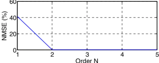
The main degree of freedom of the SEM algorithm is the choice of the order N appearing in (2). Indeed, since the number of poles needed to accurately model the signal is not known a priori, this parameter has to be chosen very carefully. One way to determine the right value is to compute the Normalized Mean Square Error (NMSE) of the reconstructed signal for different N values. This is done for 1 ≤ N ≤ 5 in Fig. 2.
Fig. 2. NMSE of the reconstructed ACGF as a function of the order N.
-1 -0.5 0 0.5 1 -1 -0.5 0 0.5 1 Position/λ AC G F mag real imag 1 2 3 4 5 0 20 40 60 Order N N M SE ( % )
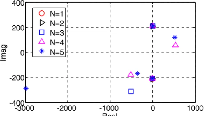
We can see that for N = 1, the NMSE is very high, meaning that one pole is not enough to model the ACGF. Then, for N ≥ 2, the NMSE is very close to zero, i.e. minor than 0.03 %. From this analysis, it seems that two poles are enough to accurately model this ACGF. The poles extracted for these different N values are presented in the complex plane in Fig. 3.
Fig. 3. Poles extracted from the 2λ-long dipole’s ACGF for various values of the order N.
For any N ≥ 2, two poles are extracted in the same way, i.e. imaginary parts close to 200 in magnitude and real parts close to zero. Some other poles are also extracted and vary from one value of N to another. Thus, this means that two poles are consistent regarding N while the other extracted seem irrelevant because changing for each different N. The residues associated to these poles are presented in the complex plane in Fig. 4.
Fig. 4. Residues linked to the poles extracted from the 2λ-long dipole’s ACGF for various values of the order N.
The residues related to the two main stable poles are quite stable as well regarding N. They obviously may change a bit because of the presence of extra poles but in general tend to stay within the same order of magnitude. Finally, the residues linked to the poles that vary with N are lower in magnitude. From all these results, we can say that two poles are necessary and enough to accurately model the ACGF of this dipole antenna.
III. RECEIVED CURRENT COMPUTATION USING ACGF In this part, we present a validation of the ACGF formalism as well as an accuracy study of the impact of the SEM modelling. Let us consider a λ/2-long dipole as presented in Fig. 5.
Fig. 5. Dipole antenna represented in a 3D space.
The ACGF of this dipole is first computed using a full-wave analysis. Then, it is excited by a plane full-wave coming from different directions and the received current is both simulated and computed using the ACGF formalism and (1). The current is also computed using the ACGF approximated by the SEM process (two poles). These three computed currents are presented as a function of θ in Fig. 6. We can see that the three curves are overlapped. This validates the ACGF formalism as well as the accuracy of the SEM modelling.
Fig. 6. Dipole antenna represented in a 3D space. REFERENCES
[1] Mikki, Said M. and Antar, Yahia M. M., “The Antenna Current Green's Function Formalism—Part I”, IEEE Transaction on Antennas and
Propagation, vol. 61, no. 9, pp 4493-4504, Sep 2013.
[2] Mikki, Said M. and Antar, Yahia M. M., “The Antenna Current Green's Function Formalism—Part II”, IEEE Transaction on Antennas and
Propagation, vol. 61, no. 9, pp 4505-4519, Sep 2013.
[3] T.K. Sarkar and O. Pereira, “Using the Matrix Pencil method to estimate the parameters of a sum of complex exponentials,” IEEE Antennas and
Propagation Magazine, vol. 37, pp 45-55, Feb. 1995.
[4] F. Sarrazin, J. Chauveau, P. Pouliguen, P. Potier and A. Sharaiha, “Accuracy of singularity expansion method in time and frequency domains to characterize antennas in presence of noise,” IEEE
Transactions on Antennas and Propagation, vol. 62, no 3, pp.
1261-1269, 2014. -3000 -2000 -1000 0 1000 -400 -200 0 200 400 Real Im a g N=1 N=2 N=3 N=4 N=5 -0.6 -0.4 -0.2 0 0.2 0.4 -0.1 -0.08 -0.06 -0.04 -0.02 0 0.02 Real Im a g N=1 N=2 N=3 N=4 N=5 0 20 40 60 80 100 0 0.05 0.1 0.15 Angle θ R e c e ive d cu rr e n t, A Wipld ACGF ACGF-SEM