Titre:
Title:
Calibration of thermal response test (TRT) units with a virtual
borehole
Auteurs:
Authors:
Alexia Corcoran, Parham Eslami-Nejad, Michel Bernier et Messaoud
Badache
Date: 2019
Type:
Article de revue / Journal articleRéférence:
Citation
:
Corcoran, A., Eslami-Nejad, P., Bernier, M. & Badache, M. (2019). Calibration of thermal response test (TRT) units with a virtual borehole. Geothermics, 79, p. 105-113. doi:10.1016/j.geothermics.2018.12.013
Document en libre accès dans PolyPublie
Open Access document in PolyPublieURL de PolyPublie:
PolyPublie URL: https://publications.polymtl.ca/3962/
Version: Version finale avant publication / Accepted versionRévisé par les pairs / Refereed Conditions d’utilisation:
Terms of Use: CC BY-NC-ND
Document publié chez l’éditeur officiel
Document issued by the official publisher Titre de la revue:
Journal Title: Geothermics (vol. 79) Maison d’édition:
Publisher: Elsevier URL officiel:
Official URL: https://doi.org/10.1016/j.geothermics.2018.12.013 Mention légale:
Legal notice:
Ce fichier a été téléchargé à partir de PolyPublie, le dépôt institutionnel de Polytechnique Montréal
This file has been downloaded from PolyPublie, the institutional repository of Polytechnique Montréal
1
Calibration of thermal response test (TRT) units
with a virtual borehole
by
Alexia Corcoran
Département de génie mécanique
Polytechnique Montréal
Intern at CanmetENERGY
Parham Eslami-Nejad
1CanmetENERGY Natural Resources Canada
Michel Bernier
Département de génie mécanique
Polytechnique Montréal
Messaoud Badache
CanmetENERGY Natural Resources Canada
Accepted manuscript
1 Corresponding author
2
Calibration of thermal response test (TRT) units
with a virtual borehole
Abstract
This paper presents the development of a virtual borehole (VB) used to calibrate the ground thermal conductivity obtained from thermal response test (TRT) units. The VB is composed of an aboveground plate heat exchanger and chiller unit carefully controlled to mimic the thermal behavior of the ground by reproducing the time evolution of the mean fluid temperature for a user-selected ground thermal conductivity. During calibration, TRT units are connected to the VB just like if they were connected to a real borehole.
The various components of the VB are described including the characterization of the heat exchanger, the implementation of a resistance-capacitance (RC) borehole model, and the required control algorithm. The VB concept is successfully tested by comparing the results obtained on a real borehole to those given by the VB for given conditions. An uncertainty analysis reveals that the ground thermal conductivity set by the VB is accurate to within ± 2.5%.
The usefulness of the VB is then demonstrated by calibrating a commercially available TRT unit for two ground thermal conductivities, 1.0 and 3.0 W m-1 K-1. Results of this calibration indicate that the TRT unit
evaluates ground thermal conductivities of 1.02 and 3.18 W m-1 K-1, respectively.
3
1.
Introduction
One of the barriers to the widespread use of ground-coupled heat pump (GCHP) system is the relatively high initial cost of the ground heat exchangers. An accurate measurement of the ground thermal conductivity reduces possible over-sizing of the bore field and therefore contributes to the development of GCHP designs that are financially competitive. The ground thermal conductivity is typically measured using a so-called thermal response test (TRT)units(Sanner et al., 2005). Other alternative methods have also been reported for in-situ thermal conductivity measurements (ASHRAE, 2007; Gehlin and Hellström, 2003; Rohner et al., 2005 and Zhang et al., 2014).
For standard tests, TRT packaged units are typically transported on site and connected to a borehole to evaluate the ground thermal conductivity. The test consists of measuring the time evolution of the mean temperature of a fluid flowing at a constant rate in the borehole while subjected to a constant heat injection rate. Guidelines for the test procedure are given by ASHRAE (2007)and Gehlin and Spitler (2003). Detailed descriptions of TRT units are found in a number of studies including those of Zhang et al., (2014); Raymond et al., (2011) and Gehlin (1998). Several TRT tests have been analysed and reported in Esen and Inalli (2009), Raymond et al. (2016), Sharqawy et al. (2009), Wu et al. (2016), and Zhou et al. (2017), to name only a few.
1.1.
TRT results interpretation
The first experimental method for determining the ground thermal conductivity and the thermal resistance between the heat transfer fluid and the borehole wall was suggested in 1983 by Mogensen (Mogensen, 1983). Since then, different mathematical models have been developed to represent boreholes in the context of TRTs. These models use either analytical or numerical approaches. The simplest and most widely used model is based on the infinite line source (ILS) analytical solution. This model assumes a constant heat injection rate into an infinite and homogeneous medium from a line along the
4 vertical axis of the borehole (Carslaw and Jaeger, 1959). A simple mathematical development (see Gehlin, 2003 or Witte, 2016) leads to an equation for the mean fluid temperature, 𝑇𝑓:
𝑇𝑓(𝑡) = 𝑄 4𝜋𝑘𝐿[𝐸1( 𝑟𝑏2 4𝛼𝑡)] + 𝑄 𝐿∙ 𝑅𝑏+ 𝑇𝑔 (1)
In this equation, 𝑘 and 𝛼 are, respectively, the ground thermal conductivity (in W m-1 K-1) and thermal
diffusivity (in m2/s), 𝑡 is the time (in s), 𝑇
𝑔 is the initial ground temperature (in °C), 𝑄 is the heat injection
rate (in W), 𝐿 is the borehole length (in m), 𝑟𝑏 is the borehole radius (in m), 𝑅𝑏 is the equivalent borehole
thermal resistance (in m K W-1) and E
1 is the exponential integral. The latter can be approximated as follows
for large values of αt/r2:
𝐸1(𝑟2
4𝛼𝑡) ≈ ln ( 4𝛼𝑡
𝑟2) − 𝛾 (2)
where 𝛾, Euler's constant, takes the value of 0.5772. This approximation leads to maximum errors of 2.5% and 10% when αt/r2 is greater than 20 and 5, respectively. The time evolution of the mean fluid
temperature in the borehole can then be written as:
𝑇𝑓(𝑡) = 𝑄 4𝜋𝑘𝐿[ln ( 4𝛼𝑡 𝑟𝑏2) − 𝛾] + 𝑄 𝐿∙ 𝑅𝑏+ 𝑇𝑔 (3)
With a constant heat injection rate 𝑄, equation (3) can be simplified to:
𝑇𝑓(𝑡) = 𝑚 ∙ ln 𝑡 + 𝑏 (4)
Where the ground thermal conductivity can then be expressed as a function of the slope 𝑚 as follows:
𝑘 = 𝑄
4𝜋𝐿𝑚 (5)
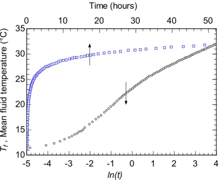
Figure 1 shows a typical time evolution of the mean fluid temperature in a borehole during an actual TRT (Beier et al., 2011). The data are plotted as a function of time (top axis) and as a function of the natural
5 logarithm of time (bottom axis). The figure shows two distinct behaviours. During the first 10 hours (𝑙𝑛(𝑡)< 2.3), the system is in a transient state where fluid and grout thermal capacities affect the mean fluid temperature. During the following hours, the system enters a quasi-steady state where transient effects in the borehole are negligible. In this region, the increase in mean fluid temperature translates into a straight line when plotted as a function of the natural logarithm of time as shown on Figure 1. The equation and the slope of this line are given by equations (3) and (5), respectively.
Fig. 1. Typical time evolution of the mean fluid temperature during a TRT.
The ILS model used for these two equations is simple, but it has shortcomings. First, the one-dimensional assumption of radial heat flow does not take into account axial heat transfer occurring near borehole extremities (Rainieri et al., 2011). Also, heat transfer inside the borehole and groundwater movement are not considered in the ILS model (Esen and Inalli, 2009 and Signorelli et al., 2007). Finally, the ILS model, as defined in equations (3) to (5), does not take into account variations in heat injection rate that can occur during TRTs (Signorelli et al., 2007). Despite these limitations, the ILS model is a robust tool still used today, as reported by Esen and Inalli (2009) and Sharqawy et al., (2009).
-5 -4 -3 -2 -1 0 1 2 3 4 10 15 20 25 30 350 10 20 30 40 50 ln(t) Tf , M ea n flu id te m pe ra tu re (° C ) Time (hours)
6 Another analytical method often used is the infinite cylinder source (ICS). This model applies the heat transfer rate at the borehole wall and thus allows a better representation of the borehole geometry than the ILS (Rainieri et al., 2011). Kavanaugh and Rafferty suggested an iterative method coupled with the ICS model to estimate the ground thermal conductivity and its thermal diffusivity (Kavanaugh and Rafferty, 1997). More recently, Fujii et al., (2009) used the ICS model and measured the axial variation in temperature with a fiber optic technology.
One, two and three-dimensional numerical models are more complex than analytical methods, but they take into account the presence of pipes and grout and also support variations in the heat injection rate (Spitler and Gehlin, 2015). These models are often coupled with a parameter estimation approach, which consists in adjusting ground thermal properties and borehole characteristics until the error between the numerical model and the experimental data obtained by a TRT is minimized (Spitler and Gehlin, 2015). For example, Bozzoli et al., (2011) developed a three-dimensional model coupled with a two-step parameter estimation procedure to determine simultaneously the ground thermal conductivity and volumetric thermal capacity. Marcotte and Pasquier (2008) built a three-dimensional borehole model that led to a new definition of the mean fluid temperature and a better estimate of the effective borehole thermal resistance.
1.2.
Review of TRT tests
In addition to developing mathematical models and parameter estimation approaches, several TRT studies have focused on improving procedures of analyzing TRT results. For example, Borinaga-Treviño et al., (2013) analyzed the inconsistency of the measured thermal conductivity when different grouts are used. Raymond et al., (2011) showed that the methodology used in standard pumping tests performed in hydrogeology can be adopted in thermal response tests.
7 Javed et al., (2011) used nine closely spaced boreholes to check random errors between tests and borehole completion methods. They concluded that the measured ground thermal conductivity has noticeable random variations. The ground thermal conductivity values for the nine boreholes lie within ±7% of the mean value.
A number of researchers have also studied the uncertainty associated with thermal response tests. Sensor errors, insufficient test duration, variable surface conditions, fluctuations of the heat injection rate, and impact of ground water are the most important factors influencing the results of a TRT.
Witte (2013) completed a thorough error analysis of TRT tests. He noted that the difference between the real value of the thermal conductivity and the estimated value is a complex combination of sensor measurement error, parameter errors (such as borehole length or fluid density), propagation of the individual errors and the error on the model itself.
Gustafsson (2006) performed a multi-injection rate thermal response test to investigate the convective currents in groundwater filled borehole heat exchangers. Witte (2013) and Chiasson and O’Connell (2011) proposed further developments in the analysis procedures of TRTs under the presence of groundwater flow.
The duration of a thermal response test has also been the subject of several investigations. Signorelli et al., (2007) studied the start and end times of thermal response tests as well as the influence of groundwater movement and borehole depth. Beier and Smith (2003) developed a graphical method to evaluate the minimum time required to estimate the ground thermal conductivity within 10% of its long-term estimation. An alternative method to delong-termine the minimum test duration is presented by Raymond (2011). Bujok et al., (2014) investigated the effect of test duration on the precision of the ground thermal conductivity and borehole resistance. Signorelli et al., (2007) compared the results obtained from a 3-D
8 finite element numerical model with those of a simple analytical line source solution and examined the test duration sensitivity.
In summary, all studies agreed that the test duration of TRT must be sufficiently long to provide a valid estimation for ground thermal conductivity. However, the minimum duration of a TRT is still under close research scrutiny and subject of on-going debate. For example Gehlin (1998) recommended a 60-hour test; Austin et al., (2000) suggested a 50-hour test , while according to ASHRAE, tests should last from 36 to 48 hours (ASHRAE, 2007). Pasquier (2018) obtained good estimates of the ground thermal conductivity using the time derivative of fluid temperature to interpret the first hours (3 hours) of a TRT.
Climatic conditions affect the connecting pipes between test equipment and sometimes the upper part of the GHE in the ground (Zhang et al., 2014). If possible, TRTs should be performed at an ambient temperature close to the fluid temperature (Ouzzane et al., 2016). Bandos et al., (2011) and Roth et al., (2004) presented correction methods to account for heat losses to the ambient.
The heat injection rate is typically assumed constant when performing a TRT test. However, it is rarely the case, since the supplied electricity voltage may vary over the course of the test. Spitler and Gehlin (2015) proposed to use active control of the heat input to maintain a relatively uniform heat input.
Ultimately, one must be able to examine the effect of different factors from the models and analytical procedures to various test conditions. Beier et al., (2011)generated a reference dataset for a two-pipe (one U-tube) 18 m long borehole installed indoors in a large sandbox under controlled conditions. Independent measurements of the sand thermal conductivity were carried out. This reference database could possibly be useful to test TRT units. However, the reduced borehole length might not be sufficient to generate a significant temperature difference with a reasonable power input. Similarly, Salim-Shirazi and Bernier (2014) built a small-scale sand tank with known thermal conductivity but it is too small to reproduce real installations.
9 Even though inter-TRT-unit comparisons have been made (Sanner et al., 2005), it is clear from this literature survey that no attempt has been made to calibrate TRT units under various ground thermal conductivities. In addition, there is no “reference” ground with known characteristics. This paper proposes a new approach, based on the concept of an aboveground virtual borehole. The primary objective of this new device is to calibrate TRT units for different user-selected ground thermal conductivities.
In the first part of the paper, the various components of the VB are described including the characterization of the plate heat exchanger and the implementation of a resistance-capacitance (RC) borehole model with its associated controlled algorithm. The VB is then tested by comparing the results obtained on a TRT carried out on an actual geothermal borehole to those given by the VB. Finally, the VB is set to reproduce ground thermal conductivities of 1.0 and 3.0 W m-1 K-1 to calibrate a commercially available TRT unit.
2.
Methodology
2.1.
Description of the virtual borehole concept
The virtual borehole is composed of aboveground equipment carefully controlled to mimic the thermal behavior of the ground by reproducing the time evolution of the mean fluid temperature in a borehole for a user-selected ground thermal conductivity.
10
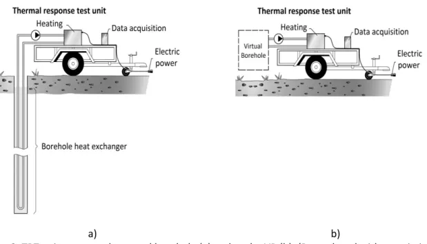
a) b)
Fig. 2. TRT unit connected to a real borehole (a) and to the VB (b). (Reproduced with permission, Gehlin and Hellström, 2003, Illustrator: Claes-Göran Andersson).
As shown in Figures 3 and 4, the VB consists of a plate heat exchanger, a cold water loop cooled by a chiller and a number of measuring instruments (see Table 1). The hot water loop is connected to the TRT unit under evaluation whereas the cold water loop represents the ground heat extraction process.
Fig. 3. Schematic representation of the virtual borehole.
TRT unit to
evaluate
Plate heat
exchanger
Chiller
F
Flowmeter
Thermopile
FFlowmeter
Thermopile
TRTin
TRTout
TCout
TCin
RTD RTD RTD RTDVirtual borehole
11
Fig. 4. Virtual borehole test bench (numbers correspond to instruments described in Table 1).
2.2.
Main variables and governing equations
As shown in Figure 3, four temperatures, 𝑇𝑅𝑇𝑖𝑛, 𝑇𝑅𝑇𝑜𝑢𝑡, 𝑇𝐶𝑖𝑛 and 𝑇𝐶𝑜𝑢𝑡, are measured on the test bench.
They represent temperatures at the inlet and outlet of the plate heat exchanger on the hot (TRT loop) and cold sides (chiller loop), respectively. The mean fluid temperatures on the TRT and chiller loops, 𝑇𝑅𝑇𝑚 and 𝑇𝐶𝑚 , are given by:
𝑇𝑅𝑇𝑚 = 𝑇𝑅𝑇𝑖𝑛+𝑇𝑅𝑇𝑜𝑢𝑡
2 (6)
𝑇𝐶𝑚 = 𝑇𝐶𝑖𝑛+𝑇𝐶𝑜𝑢𝑡
2 (7)
The chiller outlet temperature, 𝑇𝐶𝑖𝑛, is controlled based on the mean temperature of the hot water loop, 𝑇𝑅𝑇𝑚, and the efficiency of the plate heat exchanger (PHE). Since the PHE is well insulated, the heat extracted from the hot water loop, 𝑄𝑇𝑅𝑇, is assumed to be equal to the heat injected into the cold water
loop, 𝑄𝑐ℎ𝑖𝑙𝑙𝑒𝑟.
𝑄𝑇𝑅𝑇= 𝑄𝐶ℎ𝑖𝑙𝑙𝑒𝑟 = 𝑄 (8)
An energy balance on the hot and cold water loops leads to:
12 𝑄𝑇𝑅𝑇= 𝑚̇𝑇𝑅𝑇∙ 𝑐𝑝,𝑇𝑅𝑇∙ (𝑇𝑅𝑇𝑖𝑛− 𝑇𝑅𝑇𝑜𝑢𝑡) (9)
𝑄𝐶ℎ𝑖𝑙𝑙𝑒𝑟 = 𝑚̇𝐶ℎ𝑖𝑙𝑙𝑒𝑟∙ 𝑐𝑝,𝐶ℎ𝑖𝑙𝑙𝑒𝑟∙ (𝑇𝐶𝑜𝑢𝑡− 𝑇𝐶𝑖𝑛) (10)
Where 𝑚̇ and 𝑐𝑝 represent the water mass flowrate and specific heat capacity in either the hot (TRT) or
cold (chiller) loops, respectively. The heat exchanger efficiency, 𝜀, is defined as follows:
𝜀 = 𝑄
𝑄𝑚𝑎𝑥 (11)
Where 𝑄𝑚𝑎𝑥 is the maximum possible heat transfer:
𝑄𝑚𝑎𝑥= min (𝑚̇𝑇𝑅𝑇∙ 𝑐𝑝,𝑇𝑅𝑇 , 𝑚̇𝐶ℎ𝑖𝑙𝑙𝑒𝑟∙ 𝑐𝑝,𝐶ℎ𝑖𝑙𝑙𝑒𝑟) ∙ (𝑇𝑅𝑇𝑖𝑛− 𝑇𝐶𝑖𝑛) (12)
The PHE efficiency has been determined experimentally and results are presented in Appendix A.
A model is needed to generate the time evolution of 𝑇𝑅𝑇𝑚 for given borehole and ground characteristics. This is accomplished using a hybrid approach where the transient behavior inside the borehole is modeled using a resistance-capacitance (RC) model while the analytical solution of the infinite cylinder source is used to model ground heat transfer outside of the borehole (Godefroy, 2014 and Godefroy and Bernier, 2014). The two-dimensional RC model is used with a one minute time step and ten axial nodes in the TRNSYS environment and it has been successfully validated against experimental data (Godefroy et al., 2016). It should be noted that other borehole models could be used with the proposed VB concept. In fact, preliminary work indicated that even the 1D infinite line source (without borehole capacity effects) could be used satisfactorily. Higher order models (e.g. 3D models with heterogonous ground conditions) could also be used to calculate the time evolution of 𝑇𝑅𝑇𝑚.
Once the time evolution of 𝑇𝑅𝑇𝑚 is obtained using the RC model, 𝑇𝑅𝑇𝑖𝑛 can be calculated using equations (6) and (9). Then, assuming that 𝑄 and the mass flow rates in the loops are constant, the time evolution of 𝑇𝐶𝑖𝑛 can be obtained as follows:
13
𝑇𝐶𝑖𝑛= 𝑇𝑅𝑇𝑖𝑛− 𝑄
𝜀∙min (𝑚̇𝑇𝑅𝑇∙𝑐𝑝,𝑇𝑅𝑇 ,𝑚̇𝐶ℎ𝑖𝑙𝑒𝑟∙𝑐𝑝,𝐶ℎ𝑖𝑙𝑙𝑒𝑟)
(13)
Alternatively, it would also be possible to control the amount of heat transferred in the PHE by varying the flow rate on the chiller side and keeping 𝑇𝐶𝑖𝑛 constant or by using a hybrid scenario. In this scenario,
𝑇𝐶𝑖𝑛 is varied while the flow rate is kept constant in the beginning of the test and then 𝑇𝐶𝑖𝑛 is kept
constant while the flow rate is varied for the rest of the test. The advantages of these two other control scenarios were examined by Eslami-Nejad et al. (2018).
The control scenario used here is to vary 𝑇𝐶𝑖𝑛 while keeping the flow rate constant throughout the test.
Equations (6) to (13) are used to calculate the time evolution of 𝑇𝐶𝑖𝑛 to be imposed on the cold water loop based on the time evolution of 𝑇𝑅𝑇𝑚 given by the RC model for a given ground thermal conductivity.
2.3.
Virtual borehole operation
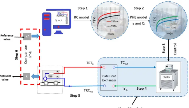
The complete operating sequence of the VB is presented in Figure 5. In step 1, the RC model is used to obtain 𝑇𝑅𝑇𝑚 as a function of time for a given set of borehole and ground characteristics, heat injection
rate and mass flow rate. The reference ground thermal conductivity, 𝑘∗, to be simulated is set in this step. Then, in step 2, the time evolution of 𝑇𝐶𝑖𝑛 is calculated according to the PHE efficiency, the mass flow rate of the cold water loop and the desired time evolution of 𝑇𝑅𝑇𝑚.
In step 3, the temperature is set in the cold water loop by controlling the chiller water outlet temperature to follow precisely the pre-calculated values of 𝑇𝐶𝑖𝑛. This is accomplished using a temperature control software within the chiller unit which allows to prescribe a set of 100 discrete values to represent the time evolution of 𝑇𝐶𝑖𝑛.
When the TRT unit and the chiller are in operation, the TRT loop reproduces the desired time evolution of the mean temperature in the hot water loop (𝑇𝑅𝑇𝑚) via the PHE (Step 4). In step 5, the TRT unit analyses the values of 𝑇𝑅𝑇𝑖𝑛 and 𝑇𝑅𝑇𝑜𝑢𝑡 to obtain a measured value of the ground thermal conductivity. Finally,
14 in step 6, the reference and measured value of thermal conductivity are compared to assess the validity of TRT results.
Fig. 5. Virtual borehole operation.
2.4.
Instrumentation and tests carried out on the virtual borehole
Devices and measuring instruments used on the virtual borehole test bench are listed in Table 1. As shown in Figure 3, four RTD probes measure the inlet and outlet temperatures of the PHE and two thermopiles (used in VB commissioning and the PHE characterization) measure the temperature difference across each water loop. Flow rates on both loops are measured using Coriolis mass flowmeters. The cold water loop has a 3-way valve to allow for flow control instead of temperature control in the cold water loop. However, this option was not used in the tests presented in this paper.
15
Table 1
Devices and measuring instruments used on the VB test bench
Element
Corresponding number on
Fig.4
Function Technical specification Uncertainty
TRT unit
Heat injection and water pumping in the hot water
loop
4 kW heating capacity
-
Chiller
Heat extraction and water pumping in the cold water
loop
5 kW cooling capacity
at 0 °C -
Plate heat
exchanger
Heat transfer between
the two water loops 0.74 m2 -
RTD
Temperaturemeasurement Pt100 ±0.1 °C
Thermopile
Differential temperaturemeasurement - ±0.007 °C
Flowmeter
Mass flow measurement Coriolis flowmeter ±0.2%In this paper, tests carried out on the VB fall into two categories: i) validation of the VB concept ii) and calibration of a TRT unit for two different thermal conductivities (1.0 and 3.0 W m-1 K-1). The parameters
used for these three tests are given in Table 2.
The pre-test procedure include the following steps:
1. Water is circulated in both circuits for a certain period before starting the test.
2. TCin is set to the undisturbed ground temperature while the heating elements of the TRT unit is
off.
3. The mass flow rates in the two circuits (𝑚̇𝑐, 𝑚̇𝑇𝑅𝑇) are adjusted to the values used in the
16
Table 2
Parameters used for the VB tests
VB Concept validation TRT unit calibration
Test 1 Test 2
Injected heat (W) 4000 4000 4000
Borehole length (m) 61.55 80 80
Mass flowrate (kg/s) 0.257 0.200 0.200
Borehole diameter (m) 0.089 0.089 0.089
Pipe outer diameter (m) 0.0267 0.0267 0.0267
Pipe inner diameter (m) 0.0218 0.0218 0.0218
Shank spacing (m) 0.015 0.0137 0.0137
Ground thermal conductivity (W m-1 K-1) 2.65 1.0 3.0
Ground thermal capacity (kJ m-3 K-1) 2415 2415 2415 Grout thermal conductivity (W m-1 K-1) 0.79 1.73 1.73
Grout thermal capacity (kJ m-3 K-1) 1500 1500 1500 Pipe thermal conductivity (W m-1 K-1) 0.43 0.43 0.43
Undisturbed ground temperature (°C) 9.4 10 10
Heat exchanger efficiency (-) 0.58 0.62 0.60
3.
Results and discussion
3.1.
Virtual borehole concept validation
The first test is used to show that the VB can reproduce the thermal behavior of a real geothermal borehole. The procedure described earlier (section 2.2) is carried out to reproduce the time evolution of the mean fluid temperature measured during an actual TRT (RNCan, 2009).
The known parameters of the geothermal borehole, i.e. the inner and outer pipe diameters, pipe thermal conductivity, borehole diameter, undisturbed ground temperature, fluid mass flowrate and ground thermal properties are used as inputs into the RC model. The heat injection rate, 𝑄, used in this verification is not the same as the one used during the TRT performed in 2009 (RNCan, 2009); the borehole length in the RC model is thus adjusted so that the ratio 𝑄/𝐿 is the same as the one used during the actual test. Unknown parameters from the 2009 test, such as shank spacing, grout thermal conductivity and
17 capacitance have been adjusted in the RC model so that the time evolution of the mean fluid temperature corresponds to the one obtained during the TRT carried out in 2009.
As indicated above, the RC model coupled with the PHE model generates the time evolution of the chiller outlet water temperature (𝑻𝑪𝒊𝒏) that is needed to reproduce the desired time evolution of the mean hot
water loop temperature on the VB. A test is then launched on the VB by imposing this time evolution of 𝑻𝑪𝒊𝒏 to the chiller and by using the same flowrate (0.257 kg/s) in the hot water loop as the one used during the TRT carried out in 2009 (RNCan, 2009).
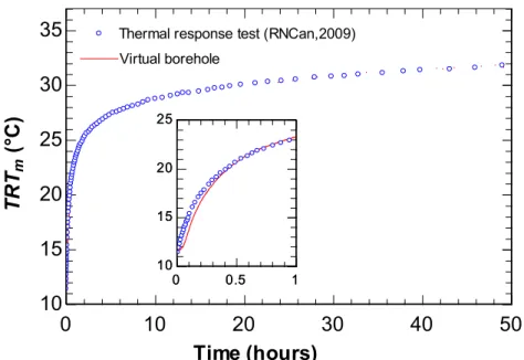
Figure 6 shows the time evolution of the mean fluid temperature during the original TRT compared to the one obtained during the test carried out on the virtual borehole. During the first 20 minutes, the mean deviation between the two curves is 0.9°C and this difference drops to an average of 0.1°C for the remaining 49.67 hours of the test. Thus, the agreement between the two curves is excellent especially after the initial transient period. This test shows that the VB test bench and its associated equipment can reproduce the ground thermal behavior during an actual TRT.
Fig. 6. Mean heat transfer fluid temperature obtained from an actual TRT (RNCan, 2009) and from the
virtual borehole. 0 0.5 1 10 15 20 25
0
10
20
30
40
50
10
15
20
25
30
35
0 0.5 1 10 15 20 25Time (hours)
TR
T
m(°
C
)
Virtual borehole Virtual boreholeThermal response test (RNCan,2009) Thermal response test (RNCan,2009)
18
3.2.
Calibration test on a TRT unit
In this section, two values of ground thermal conductivities, 1.0 W m-1 K-1 and 3.0 W m-1 K-1, are reproduced
by the VB and used to calibrate a commercially available TRT unit. Parameters for both tests (Table 2) are identical with the exception of the ground thermal conductivity and the PHE efficiency. The latter is not the same for both tests since it is calculated according to the temperature range of 𝑇𝐶𝑖𝑛 during the test, which differs according to the ground thermal conductivity to be simulated (see Appendix A). A heat injection rate of 4 kW is used in the RC model simulations since this is the power used by TRT unit under calibration.
The time evolutions of the mean fluid temperatures and of the chiller outlet water temperature (𝑇𝐶𝑖𝑛) are obtained from the RC model and entered as 100 discrete values in the chiller control algorithm. Then, the flow rates are set to 0.200 kg/s in both loops and heat injection from the TRT unit is initiated. Finally, as shown in Table 3, both tests performed by the TRT unit comply with ASHRAE recommendations (ASHRAE, 2007).
Table 3
Compliance of the VB tests with ASHRAE recommendations for TRT (ASHRAE, 2007).
Tests on the VB ASHRAE recommandations 𝑘 = 1.0 W m-1 K-1 𝑘 = 3.0 W m-1 K-1
Time Data acquisition interval
(s) 2 2 ≤ 600
Heat transfer fluid temperature
Temperature difference
(°C) 4.74 4.74 3.3 to 6.7
Heat injection
Standard deviation from the average power
level (%)
1.5 1.5 ≤ 1.5
Peak deviation from the average power level
(%)
7.7 7.9 ≤ 10
Heat injection rate
19 Figures 7 and 8 show the time evolutions of the measured 𝑇𝑅𝑇𝑚 on the VB and the corresponding value
predicted by the RC model for the two ground thermal conductivities.
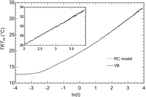
Fig. 7. Comparison between the measured values of 𝑇𝑅𝑇𝑚 and the ones predicted by the RC model
for 𝑘 = 1.0 W m-1 K-1.
Fig. 8. Comparison between the measured values of 𝑇𝑅𝑇𝑚 and the ones predicted by the RC model for 𝑘 = 3.0 W m-1 K-1. 2 2.5 3 3.5 26 28 30 32 34 -4 -3 -2 -1 0 1 2 3 4 10 15 20 25 30 35 2 2.5 3 3.5 26 28 30 32 34 ln(t) TR Tm (° C ) VB VB RC model RC model 2 2.5 3 3.5 20 21 22 23 24 -6 -5 -4 -3 -2 -1 0 1 2 3 4 12 14 16 18 20 22 24 2 2.5 3 3.5 20 21 22 23 24 ln(t) TR Tm (° C ) RC model RC model VB VB
20 As shown in these Figures, the time evolution of 𝑇𝑅𝑇𝑚 obtained on the virtual borehole is very similar to that given by the RC model. For 𝑘 = 1.0 W.m-1.K-1, the maximum deviation between the experimental curve
and the RC curve is 0.3°C and the mean deviation is 0.09°C. The maximum deviation occurs within the first minute of the test and is caused by the hot water loop temperature that is initially not exactly the same as the one calculated by the RC model. After a few minutes, the temperature of the hot water loop approaches the one predicted by the RC model and the gap between the curves decreases. For 𝑘 = 3.0 W.m-1.K-1, the maximum deviation between the curves is 0.4°C and the mean deviation is
0.07°C. In this case, the maximum deviation occurs 6 minutes after the start of the test. It is exactly at this time that the rate of change in the chiller outlet temperature is the highest. Thus, the chiller reaches the desired output temperature with a delay. Based on these results, the VB is thus able to successfully reproduce the ground thermal behavior predicted by the RC model for ground thermal conductivities of 1.0 W.m-1.K-1 and 3.0 W.m-1.K-1.
The TRT unit connected to the virtual borehole has its own set of measurements and it records temperature, flow, current and voltage. The data recorded in the TRT unit’s acquisition system is exported to an analysis software within the TRT unit. The initial transient period, assumed to be 20 hours in this case, is excluded from the analysis. Then, the infinite line source method is used by the TRT software to calculate the ground thermal conductivity resulting from the data obtained by the TRT unit.
Table 4
Summary of results obtained on the calibration of a TRT unit with the VB
VB TRT unit
Ground thermal
conductivity set in the VB Uncertainty1
Ground thermal conductivity calculated by the TRT unit Difference between VB and TRT unit 1.00 W.m-1.K-1 ±2.7% 1.02 W.m-1.K-1 2% 3.00 W.m-1.K-1 ±2.7% 3.18 W.m-1.K-1 6% 1 discussed in section 3.3
21 For the two tests performed using the virtual borehole, the analysis software calculated thermal conductivities of 1.02 and 3.18 W.m-1.K-1, respectively. This corresponds to differences of 2% and 6%,
respectively, when compared to the values set by the VB. Table 4 summarised these results.
3.3.
Uncertainty analysis
The ground thermal conductivity uncertainty simulated by the virtual borehole is assessed in this section. Two different approaches are used: the first one determines the absolute uncertainty for a given test and the second one estimates the maximum test uncertainty.
The first approach consists in modifying the ground thermal conductivity in the RC model until the root mean square error between the 𝑇𝑅𝑇𝑚 time evolution obtained on the VB during the test and the one prescribed by the RC model is minimized. The difference between the ground thermal conductivity which minimizes the root mean square error and the thermal conductivity which was initially simulated represents the absolute uncertainty for the test performed. This absolute uncertainty is specific to one ground thermal conductivity and to one test. Using this approach, an uncertainty of ±0.005 W m-1 K-1 is
found for both calibration tests. This uncertainty corresponds to relative uncertainties of ±0.5% and ±0.2% for the 1.0 W.m-1.K-1 and 3.0 W.m-1.K-1 tests, respectively.
The second approach consists in applying the classic uncertainty propagation method to the infinite line source (ILS) equation to determine the maximum uncertainty that can be encountered during a test for a given thermal conductivity. The ILS method is used here as a proxy to determine the uncertainty. The ILS equation can be expressed as:
𝑘 = 𝑄 4𝜋𝐿𝑚= 𝜀∙𝑄𝑚𝑎𝑥 4𝜋𝐿𝑚 = 𝜀∙min (𝑚̇𝑇𝑅𝑇∙𝑐𝑝,𝑇𝑅𝑇 ,𝑚̇𝐶ℎ𝑖𝑙𝑙𝑒𝑟∙𝑐𝑝,𝐶ℎ𝑖𝑙𝑙𝑒𝑟)∙(𝑇𝑅𝑇𝑖𝑛−𝑇𝐶𝑖𝑛) 4𝜋𝐿𝑚
(14)
Uncertainties on the thermal capacity of water (cp) and on the length of the simulated geothermal
22 It can be shown that the relative uncertainty on 𝑘 is given by:
𝛿𝑘 𝑘 = √( 𝛿𝜀 𝜀) 2 + (𝛿𝑚̇ 𝑚̇) 2 + (𝛿𝑇𝐶𝑖𝑛 𝑇𝐶𝑖𝑛) 2 + 3 (𝛿𝑇𝑅𝑇𝑖𝑛 𝑇𝑅𝑇𝑖𝑛) 2 + 2 (𝛿𝑇𝑅𝑇𝑜𝑢𝑡 𝑇𝑅𝑇𝑜𝑢𝑡) 2
(15)
where the symbol 𝛿 is used to represent uncertainties on the measured quantities.
The uncertainty on the mass flow rate corresponds to that stated by the manufacturer. Finally, the uncertainties used for 𝛿𝑇𝐶𝑖𝑛, 𝛿𝑇𝑅𝑇𝑖𝑛 and 𝛿𝑇𝑅𝑇𝑜𝑢𝑡 are based on calibration results of the RTD probes (see
Table 1) on the VB test bench. The chiller stability must be added to the uncertainty on 𝑇𝐶𝑖𝑛, since it is imposed by the chiller. Using equation (15), the maximum uncertainties is ±2.7%.
With results of these two uncertainty evaluation methods, the uncertainty on the values of 𝑘 given by the VB is conservatively set at ±2.7%.
4.
Conclusion and future work
This paper presents the development of a virtual borehole (VB) used to verify the ground thermal conductivity obtained from thermal response test (TRT) units. The VB consists of a plate heat exchanger, a water loop cooled by a chiller and a control algorithm. The TRT under evaluation is simply connected to the VB as it would be for a real geothermal borehole.
The temperature evolution produced in the cold water loop is interpreted by the TRT units as if it were to a real borehole in a ground of a certain thermal conductivity. To change the thermal conductivity under which TRT units are evaluated, one only needs to change the time evolution of the temperature in the cold water loop. A two-dimensional resistance-capacitance (RC) numerical model coupled with a PHE model determines this temperature evolution. An uncertainty analysis reveals that the ground thermal conductivity set by the VB is accurate to within ±2.7% when the RC model is used. One of the main assumption of the RC model is the use of homogeneous ground conditions. More work is needed with
23 higher order models that could, for example, predict the time evolution of 𝑇𝐶𝑖𝑛 for heterogeneous ground
conditions. Such models could be used in a parametric analysis to determine the limits of the VB in emulating real ground conditions.
Nonetheless, the usefulness of the VB is demonstrated by calibrating a commercially available TRT unit for two homogenous ground conditions with thermal conductivities of 1.0 and 3.0 W m-1 K-1, respectively.
Results of this calibration indicate that the TRT unit evaluates these ground thermal conductivities with errors of 2.0 and 6.0%, respectively. Thus, it appears that the TRT unit may have a problem evaluating high ground thermal conductivities, as the error is higher than the uncertainty of the VB (2.7%).
As shown in this paper, the VB concept is a viable option to calibrate TRT units. However, some additional tests over a broader range of experimental conditions are required. In particular, the plate heat exchanger needs to be characterise over the complete range of flow rates and temperatures that are likely to be used during TRTs. It would also be advantageous to include phenomena that occur during actual thermal response tests, such as power outages. The VB should also be useful in round robin testing of TRT units as it can replicate the same virtual ground conditions.
Acknowledgements
The authors would like to acknowledge the funding received by the Office of Energy Research and Development (OERD) of Canada through the ecoENERGY Innovation Initiative for test bench construction and supporting the research. Furthermore, the Natural Sciences and Engineering Research Council of Canada also provided funding through a discovery grant awarded to one of the authors. Finally, the authors would like to acknowledge Dr. Mohamed Ouzzane for his scientific and technical advice during the development of the concept and the test bench design and construction.
24
References
ASHRAE, 2007. ASHRAE Handbook. Heating, Ventilating, and Air-conditioning Applications. American Society of Heating Refrigerating and Air-Conditioning Engineers.
Austin, W.A., Yavuzturk, C., Spitler, J.D., 2000. Development of an in-situ system and analysis procedure for measuring ground thermal properties/Discussion. ASHRAE Trans. 106, 365.
Bandos, T. V, Montero, Á., Fernández de Córdoba, P., Urchueguía, J.F., 2011. Improving parameter estimates obtained from thermal response tests: Effect of ambient air temperature variations. Geothermics 40, 136–143. doi:http://dx.doi.org/10.1016/j.geothermics.2011.02.003
Beier, R.A., Smith, M.D., 2003. Symposium papers-kc-03-03: Minimum Duration of In-Situ Tests on Vertical Boreholes. ASHRAE Trans. Soc. Heat. Refrig. Airconditioning Engin 109, 475–486.
Beier, R.A., Smith, M.D., Spitler, J.D., 2011. Geothermics Reference data sets for vertical borehole ground heat exchanger models and thermal response test analysis. Geothermics 40, 79–85. doi:10.1016/j.geothermics.2010.12.007
Borinaga-Treviño, R., Pascual-Muñoz, P., Castro-Fresno, D., Blanco-Fernandez, E., 2013. Borehole thermal response and thermal resistance of four different grouting materials measured with a TRT. Appl. Therm. Eng. 53, 13–20. doi:10.1016/j.applthermaleng.2012.12.036
Bozzoli, F., Pagliarini, G., Rainieri, S., Schiavi, L., 2011. Estimation of soil and grout thermal properties through a TSPEP applied to TRT (thermal response test) data. Energy 36, 839–846.
Bujok, P., Grycz, D., Klempa, M., Kunz, A., Porzer, M., Voj, P., 2014. Assessment of the in fluence of shortening the duration of TRT ( thermal response test ) on the precision of measured values. Energy 64, 120–129. doi:10.1016/j.energy.2013.11.079
Carslaw, H.S., Jaeger, J.C., 1959. Conduction of heat in solids. Oxford Clarendon Press. 1959, 2nd ed. Chiasson, A., O’Connell, A., 2011. New analytical solution for sizing vertical borehole ground heat
exchangers in environments with significant groundwater flow: Parameter estimation from thermal response test data. HVAC&R Res. 17, 1000–1011. doi:10.1080/10789669.2011.609926
Esen, H., Inalli, M., 2009. In-situ thermal response test for ground source heat pump system in Elazıg . Energy Build 41, 395–401. doi:10.1016/j.enbuild.2008.11.004
Eslami-Nejad, P., Badache, M., Corcoran, A., Bernier, M., 2018. A virtual borehole for thermal response test unit calibration: test facility and concept development. Proceedings of the IGSHPA Research Track 2018. Stockholm, Sweden. pp. 198-206.
Fujii, H., Okubo, H., Nishi, K., Itoi, R., Ohyama, K., Shibata, K., 2009. An improved thermal response test for U-tube ground heat exchanger based on optical fiber thermometers. Geothermics 38, 399–406. doi:http://dx.doi.org/10.1016/j.geothermics.2009.06.002
Gehlin, S. , Hellström, G. 2003. Influence on thermal response test by groundwater flow in vertical fractures in hard rock. Renewable energy 28(14), 2221-2238..
Gehlin, S., 1998. Thermal Response Test: method development and evaluation. Thesis, Luleå University of Technology, ISSN 1402-1544 ; 2002:39.
Gehlin, S., Spitler, J.D., 2003. Thermal response test for BTES applications-state of the art 2001. In: 9th International Conference on Thermal Energy Storage Warsaw, Poland, pp, 381–387.
Godefroy, V. 2014. Élaboration et validation d'une suite évolutive de modèles d'échangeurs géothermiques verticaux. M.A.Sc thesis, École Polytechnique de Montréal. https://publications.polymtl.ca/1481/
Godefroy, V., Bernier, M., 2014. A simple model to account for thermal capacity in boreholes, in: 11th IEA Heat Pump Conference 2014.
Godefroy, V., Lecomte, C., Bernier, M., Douglas, M.,Armstrong, M., 2016. Experimental validation of a thermal resistance and capacity model for geothermal boreholes. ASHRAE winter conference, Orlando, Florida, January 2016. Paper OR-16-C047.
25 Gustafsson, A.M., 2006. Thermal response test: numerical simulations and analyses. Thesis, Luleå
University of Technology, ISSN 1402-1757 ; 2006:14
Javed, S., Spitler, J.D., Fahlén, P., 2011. An experimental investigation of the accuracy of thermal response tests used to measure ground thermal properties. ASHRAE Trans. 117, 13–21.
Kavanaugh, S.P., Rafferty, K., 1997. Ground-source heat pumps: design of geothermal systems for commercial and institutional buildings. ASHRAE Applications Handbook, Atlanta, GA, US.
Marcotte, D., Pasquier, P., 2008. On the estimation of thermal resistance in borehole thermal conductivity test. Renewable Energy 33, 2407–2415. doi:10.1016/j.renene.2008.01.021
Mogensen, P., 1983. Fluid to duct wall heat transfer in duct system heat storages. Document-Swedish Council for Building Research 16, 652-657.
Ouzzane, M., Badache, M., Eslami-Nejad, P., Aidoun, Z, 2016. Recent Advances in Shallow Ground Thermal Energy: Modeling and Developments. Lambert Academic Publishing 152.
ISBN-13:978-3-659-81860-8.
Pasquier, P. 2018. Interpretation of the first hours of a thermal response test using the time derivative of the temperature. Applied Energy, 213, 56-75. https://doi.org/10.1016/j.apenergy.2018.01.022 Rainieri, S., Bozzoli, F., Pagliarini, G., 2011. Modeling approaches applied to the thermal response test : A
critical review of the literature. HVAC&R Research 17, 977–990. doi:10.1080/10789669.2011.610282 Raymond, J., Therrien, R., Gosselin, L., Lefebvre, R., 2011. A Review of Thermal Response Test Analysis
Using Pumping Test Concepts. Groundwater 49, 932–945. doi:10.1111/j.1745-6584.2010.00791 Raymond, J., Lamarche, L., Malo, M., 2016. Extending thermal response test assessments with inverse
numerical modeling of temperature profiles measured in ground heat exchangers. Renewable Energy 99, 614–621. doi:http://dx.doi.org/10.1016/j.renene.2016.07.005
RNCan, 2009. Évaluation de la conductivité du sol de CanmetENERGY-Varennes. Internal TRT report, Varennes.
Rohner, E., Rybach, L., Schärli, U., 2005. A new, small, wireless instrument to determine ground thermal conductivity in-situ for borehole heat exchanger design, in: Proceedings World Geothermal Congress. Roth, P., Georgiev, A., Busso, A., Barraza, E., 2004. First in situ determination of ground and borehole thermal properties in Latin America. Renewable Energy 29, 1947–1963. doi:10.1016/j.renene.2004.02.014
Salim Shirazi, A., Bernier, M., 2014. A small-scale experimental apparatus to study heat transfer in the vicinity of geothermal boreholes. HVAC&R Res. 20, 819–827. doi:10.1080/10789669.2014.939553 Sanner, B., Hellström, G., Spitler, J., Gehlin, S., 2005. Thermal response test—current status and
world-wide application, in: Proceedings World Geothermal Congress. International Geothermal Association.
Sharqawy, M.H., Mokheimer, E.M., Habib, M.A., Badr, H.M., Said, S.A., Al-Shayea, N.A., 2009. Energy, exergy and uncertainty analyses of the thermal response test for a ground heat exchanger. Int. J. Energy Res. 33, 582–592. doi:10.1002/er.1496
Signorelli, S., Bassetti, S., Pahud, D., Kohl, T., 2007. Numerical evaluation of thermal response tests. Geothermics 36, 141–166. doi:10.1016/j.geothermics.2006.10.006
Spitler, J.D., Gehlin, S.E.A., 2015. Thermal response testing for ground source heat pump systems — An historical review. Renew. Sustain. Energy Rev. 50, 1125–1137. doi:10.1016/j.rser.2015.05.061 Witte, H., 2007. Advances in geothermal response testing. Therm. Energy Storage Sustain. Energy Consum.
177–192.
Witte, H., 2013. Error analysis of thermal response tests. Appl. Energy 109, 302–311. doi:10.1016/j.apenergy.2012.11.060
Witte, H., 2016. Advances in Ground-Source Heat Pump Systems- Chapter 4: In situ estimation of ground thermal properties. Edited by S. Rees. Woodhead (Elsevier) Publishing. ISBN: 978-0-08-100311-4 Wu, X., Wang, Z., Jin, G., Yang, X., Zhang, Z., Bi, W., 2016. Development and experimental study on testing
26 platform for rock-soil thermal response tester. Renew. Energy 87, 765–771. doi:http://dx.doi.org/10.1016/j.renene.2015.10.057
Zhang, C., Guo, Z., Liu, Y., Cong, X., Peng, D., 2014. A review on thermal response test of ground-coupled
heat pump systems. Renew. Sustain. Energy Rev. 40, 851–867.
doi:http://dx.doi.org/10.1016/j.rser.2014.08.018
Zhou, Y., Zhao, L., Wang, S., 2017. Determination and analysis of parameters for an in-situ thermal response test. Energy Build. 149, 151–159. doi:https://doi.org/10.1016/j.enbuild.2017.05.048
27
Appendix A
Plate heat exchanger characterization
A series of experiments were undertaken to determine the plate heat exchanger efficiency as a function of the inlet temperatures and flow rates. The heat exchanger efficiency is defined as follows:
𝜀 =
𝑄 𝑄𝑚𝑎𝑥=
𝑄
min (𝑚̇𝑇𝑅𝑇∙𝑐𝑝,𝑇𝑅𝑇 ,𝑚̇𝐶ℎ𝑖𝑙𝑙𝑒𝑟∙𝑐𝑝,𝐶ℎ𝑖𝑙𝑙𝑒𝑟)∙(𝑇𝑅𝑇𝑖𝑛−𝑇𝐶𝑖𝑛) (A-1)
The efficiency becomes a function only of the heat exchanger inlet temperatures 𝑇𝑅𝑇𝑖𝑛 and 𝑇𝐶𝑖𝑛 with the
following assumptions: i) 𝑄 is constant; ii) 𝑚̇𝑇𝑅𝑇 and 𝑚̇𝐶ℎ𝑖𝑙𝑙𝑒𝑟 are equal and constant; iii) 𝑐𝑝,𝑇𝑅𝑇=
𝑐𝑝,𝐶ℎ𝑖𝑙𝑙𝑒𝑟 = 4.18 kJ kg-1 K-1.
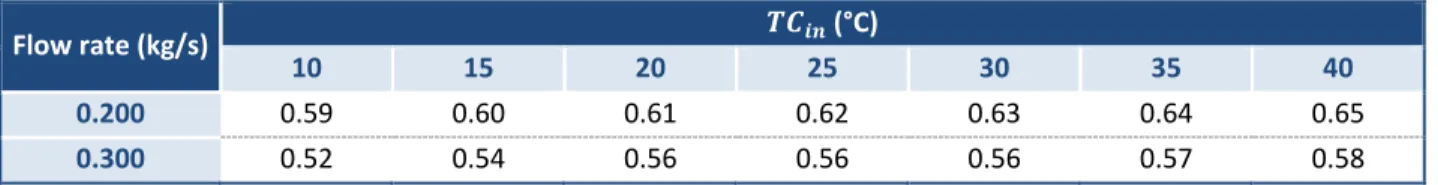
The characterization of the heat exchanger is carried under steady-state conditions for two flow rates (0.200 kg/s and 0.300 kg/s) for values of 𝑇𝐶𝑖𝑛 varying from 10°C to 40°C in 5°C increments and 4 kW heat
injection rate.
Table A-1: Plate heat exchanger efficiency as a function of 𝑻𝑪𝒊𝒏 and flow rate
Flow rate (kg/s) 𝑻𝑪𝒊𝒏 (°C)
10 15 20 25 30 35 40
0.200 0.59 0.60 0.61 0.62 0.63 0.64 0.65
0.300 0.52 0.54 0.56 0.56 0.56 0.57 0.58
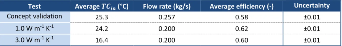
Results presented in Table A-1 show that the efficiency increases linearly with 𝑇𝐶𝑖𝑛 for a given flowrate. However, as shown in Figures 7 and 8, the use of an average and constant efficiency value in the RC model for the entire test is more than adequate to reproduce successfully the desired thermal behavior in the hot water loop. The average efficiency is calculated from the performance map presented in Table A-2 using linear interpolation according to the flow rate and mean chiller outlet water temperature (𝑇𝐶𝑖𝑛) prevailing during the entire test. The average efficiency value is not the same for the three tests carried
28 out in this paper since the average value of 𝑇𝐶𝑖𝑛 varies according to the simulated ground thermal
conductivity. Table A-2 presents these values of 𝑇𝐶𝑖𝑛 as well the flow rates for the three tests performed
and the resulting average PHE efficiency. Finally, the absolute uncertainty on the efficiency has been estimated at ±0.01 by calculating the maximum uncertainty occurring during the characterization of the PHE according to the uncertainties of the various measuring instruments used.
Table A-2: Average PHE efficiency used for the tests performed on the VB
Test Average 𝑻𝑪𝒊𝒏 (°C) Flow rate (kg/s) Average efficiency (-) Uncertainty
Concept validation 25.3 0.257 0.58 ±0.01
1.0 W m-1 K-1 24.2 0.200 0.62 ±0.01