CURE RATE MODELS
MAHROO VAHIDPOUR
DÉPARTEMENT DE MATHÉMATIQUES ET DE GÉNIE INDUSTRIEL ÉCOLE POLYTECHNIQUE DE MONTRÉAL
MÉMOIRE PRÉSENTÉ EN VUE DE L’OBTENTION DU DIPLÔME DE MAÎTRISE ÈS SCIENCES APPLIQUÉES
(MATHÉMATIQUES APPLIQUÉES) DÉCEMBRE 2016
c
ÉCOLE POLYTECHNIQUE DE MONTRÉAL
Ce mémoire intitulé :
CURE RATE MODELS
présenté par : VAHIDPOUR Mahroo
en vue de l’obtention du diplôme de : Maîtrise ès sciences appliquées a été dûment accepté par le jury d’examen constitué de :
M. LEFEBVRE Mario, Ph. D., président
M. ADJENGUE Luc-Désiré, Ph. D., membre et directeur de recherche
M. ASGHARIAN-DASTENAEI Masoud, Ph. D., membre et codirecteur de recherche Mme ATHERTON Juli , Ph. D., membre
DEDICATION
To my lovely family, you are always in my heart. . .
ACKNOWLEDGMENTS
It has been a period of intense learning during my research for masters, not only in the scientific arena, but also on a personal level. Writing this thesis has had a big impact on my training. I would like to reflect on the people who have supported and helped me throughout this period.
First, I would like to thank my thesis advisers Prof. Luc Adjengue from Mathematics and In-dustrial Engineering Department at Polythechnique University, and Prof. Masoud Asgharian from faculty of Mathematics and Statistics Department at McGill University. My supervisors consistently allowed this thesis to be my own work, but steered me in the correct direction whenever they thought I needed it.
Besides my advisers, I would particularly like to thank Prof. Vahid Partovi Nia for dedication of his time to revise this thesis and give me many critical advices. He supported me greatly and was always willing to help. I would also, here by give my many thanks to the rest of my thesis committee Prof. Mario Lefebvre from Mathematics and Industrial Engineering Department at Polythechnique University and Prof. Juli Atherton from Mathematics and Statistics Department at UQAM who were involved in the validation survey of this thesis. Without their passionate participation and input, the validation survey could not have been successfully conducted.
My sincere thanks also goes to Mr. Eric Jobin and Mr. Jean-Francois Ross From Pratt and Whitney Canada for offering me the internship opportunities in their groups and leading me working on diverse exciting statistical projects.
Finally, I must express my very profound gratitude to my parents for providing me with unfailing support and continuous encouragement throughout my years of study and through the process of writing this thesis. This accomplishment would not have been possible without their support. Thank you all.
RÉSUMÉ
Les modèles de survie avec taux de guérison ont une vaste gamme d’applications dans de nombreux domaines tels que la médecine et la santé publique, en particulier dans des études sur le cancer. Dans ces études, les chercheurs sont intéressés par le temps d’attente jusqu’à l’apparition d’un événement d’intérêt, ainsi qu’à la proportion des cas où cet événement ne survient jamais, qualifiée dans ce contexte de taux de guérison. D’une manière générale, il existe deux types de modèles pour l’estimation du taux de guérison. Le premier type est le modèle de mélange avec taux de guérison. Ce type de modèles suppose que l’ensemble de la population se compose de deux groupes d’individus : les individus susceptibles de subir l’événement d’intérêt et les individus non susceptibles de subir l’événement d’intérêt, ou immunisés. Le deuxième modèle est un modèle de non-mélange avec taux de guérison qui se base, par exemple, sur le nombre de cellules cancéreuses qui restent après le traitement. Ce mémoire conçoit et présente une revue des modèles de survie avec taux de guérison depuis les premières études jusqu’aux articles récents. Puisqu’il n’y a pas d’étude exhaustive des modèles de taux de guérison, ma mission se limitera au regroupement de tous les modèles dans une notation unique et cohérente.
Les modèles de taux de guérison font partie de l’analyse de survie et incluent les cas de censure. Par conséquent, pour une analyse convenable des modèles de taux de guérison, une bonne connaissance de l’analyse de survie est nécessaire. Ainsi, au chapitre 2, les définitions relatives aux sujets censurés et tronqués sont données. En outre, les concepts et formulations de l’analyse de survie de base sont expliqués. Des modèles de survie courants, paramétriques, non paramétriques et semi-paramétriques sont également expliqués. Les chapitres 3 et 4 forment la partie principale de ce mémoire ; ils portent essentiellement sur l’explication des modèles de taux de guérison. Au chapitre 3, des tests préliminaires pour l’existence d’un taux de guérison sont expliqués. Les premiers travaux dans les modèles de mélange avec taux de guérison et certains modèles paramétriques et non paramétriques avec taux de guérison y sont discutés. L’un des modèles de non-mélange avec taux de guérison et deux modèles de mélange semi-paramétriques qui ont été adaptés des travaux plus récents dans les modèles avec taux de guérison sont expliqués au chapitre 4.
Au chapitre 5, une étude de simulation a été effectuée pour chaque modèle introduit précédem-ment afin d’en tester la précision. Les méthodes des études de simulation sont les mêmes que celles utilisées dans les articles originaux. Au chapitre 6, les modèles avancés avec taux de guérison sont mis en œuvre pour des bases de données de transplantation de moelle osseuse et
les résultats sont discutés. Le chapitre 7 présente la conclusion de l’étude ainsi qu’un aperçu d’une future recherche.
ABSTRACT
Cure rate models have a broad range of application in many fields, such as medicine, public health, and especially in cancer studies. Researchers in these studies are interested in waiting time until occurrence of the event of interest, as well as the proportion of instances where the event never occurs, known in this case as the cure fraction. In general, there are two types of models for estimation of the cure fraction. The first one is the mixture cure rate model. This type of models assumes that the whole population is composed of two groups of subjects, susceptible subjects and insusceptible (or cured) subjects. The second model is non-mixture cure model, based on number of cancer cells which remain after treatment. This thesis devises and presents a review for cure rate models form early studies to recent articles. Since there is not a comprehensive review on cure rate models, my mission was to put all models together in a single and coherent notation.
Cure rate models are a part of survival analysis and involve censored subjects. Therefore, analyses cure rate models a sufficient knowledge in survival analysis is required. In Chap-ter 2, the definitions of censored and truncated subjects are given. In addition, the basic concepts and formulations of survival analysis are explained. Some common parametric and non-parametric, and semi-parametric survival models are explained as well.
Chapter 3 and Chapter 4 are the main body of this dissertation, and focus on explain-ing cure rate models. In Chapter 3, some preliminary tests for existence of cured fraction are described. Early works in mixture cure rate models and some parametric and non-parametric cure models are discussed. In Chapter 4 non-mixture cure rate models and two semi-parametric mixture cure rate models which are adopted from more recent works in cure models are explained.
An extensive simulation study has been done for each model type and is discussed in Chapter 5. Simulation setup is the same as in original article and we were able to reproduce their re-sults. In Chapter 6, advanced cure models are implemented for bone marrow transplantation dataset. Chapter 7 presents the conclusion of the study and an overview of future research.
TABLE OF CONTENTS
DEDICATION . . . iii
ACKNOWLEDGMENTS . . . iv
RÉSUMÉ . . . v
ABSTRACT . . . vii
TABLE OF CONTENTS . . . viii
LIST OF TABLES . . . xi
LIST OF FIGURES . . . xii
LISTE OF APPENDICES . . . xiii
CHAPTER 1 INTRODUCTION . . . 1
CHAPTER 2 SURVIVAL MODELS . . . 5
2.1 Introduction . . . 5
2.2 Censoring types and truncation . . . 5
2.2.1 Right censoring . . . 6
2.2.2 Left censoring . . . 7
2.2.3 Interval censoring . . . 7
2.2.4 Truncation . . . 7
2.3 Analysis of survival data . . . 7
2.3.1 Likelihood construction . . . 9
2.4 Survival models . . . 11
2.4.1 Nonparametric survival models . . . 11
2.4.2 Parametric survival models . . . 12
2.4.3 Semiparametric survival models . . . 14
CHAPTER 3 CURE RATE MODELS: CLASSICAL APPROACH . . . 18
3.1 Introduction . . . 18
3.2 Preliminaries . . . 18
3.2.2 Is the follow-up time long enough? . . . 21
3.3 Mixture cure rate models . . . 23
3.3.1 History . . . 23
3.3.2 Formulation of mixture models . . . 24
3.3.3 Likelihood function for mixture models . . . 26
3.4 Parametric mixture models . . . 26
3.4.1 Weibull and conditional logistic mixture model . . . 26
3.5 Nonparametric mixture models . . . 27
3.5.1 Proportional hazard mixture model . . . 28
CHAPTER 4 CURE RATE MODELS: MODERN APPROACH . . . 32
4.1 Introduction . . . 32
4.2 Semiparametric models . . . 32
4.2.1 Cure rate quantile regression mixture model . . . 32
4.2.2 Two groups trial with semiparametric method . . . 37
4.3 Non-mixture models . . . 41
4.3.1 Semi-Parametric non-mixture models . . . 42
CHAPTER 5 SIMULATION . . . 46
5.1 Introduction . . . 46
5.1.1 Cure rate quantile regression model . . . 46
5.1.2 Two groups mixture model . . . 48
5.2 Non-mixture models . . . 48
CHAPTER 6 APPLICATION . . . 51
6.1 Data summary . . . 51
6.2 Survival models . . . 52
6.2.1 Cox proportional hazard model . . . 52
6.3 Cure rate models . . . 54
6.3.1 Preliminary tests . . . 54
6.3.2 Mixture models . . . 55
6.3.3 Non-mixture model . . . 57
CHAPTER 7 CONCLUSION . . . 60
7.1 Synthesis of cure rate models . . . 60
7.2 Summary of simulation results and future work . . . 61
LIST OF TABLES
Table 2.1 Censoring schemes and the likelihood Function. . . 10
Table 5.1 Gamma estimation in cure rate quantile regression. . . 47
Table 5.2 Estimation of quantile coefficients in simulation study. . . 47
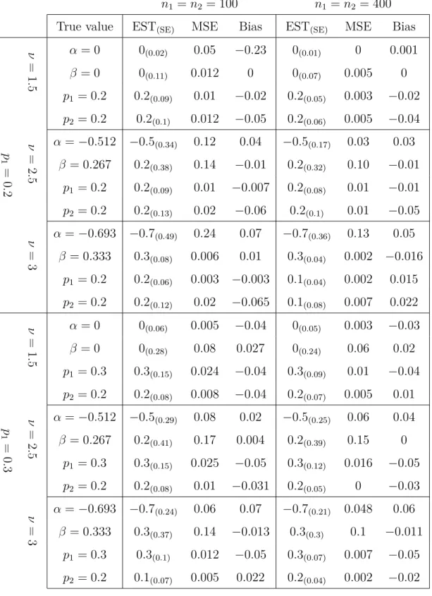
Table 5.4 Parameter estimation for non-mixture cure models. . . 49
Table 5.3 Parameter estimation for two groups mixture cure rate model. . . 50
Table 6.1 Cox proportional hazard model for bone marrow stransplant data. . . 55
Table 6.2 Cox proportional hazard cure rate model group ALL. . . . 56
Table 6.3 Cox proportional hazard cure model group AML high risk. . . . 56
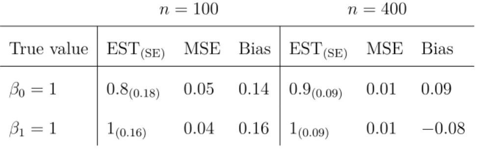
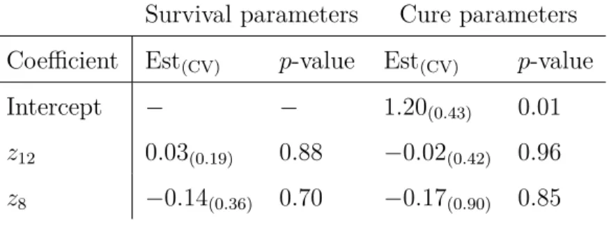
Table 6.4 Estimation of β0 in fitting cure rate quantile regression on BMT data. 57 Table 6.5 Estimation of β1 in fitting cure rate quantile regression on BMT data. 58 Table 6.6 Estimation of β2 in fitting cure rate quantile regression on BMT data. 58 Table 6.7 BMT data fitted by semiparametric two groups model. . . 58
LIST OF FIGURES
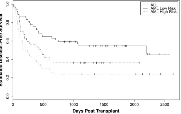
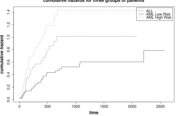
Figure 1.1 The concept diagram of cure rate models. . . 3 Figure 2.1 Censoring and truncation illustration. . . 8 Figure 3.1 Kaplan-Meier estimator. . . 19 Figure 6.1 Kaplan-Meier estimate for each group of patients in BMT dataset. . . 53 Figure 6.2 Cumulative hazard estimate for each group of patients in BMT dataset. 54
LISTE OF APPENDICES
APPENDIX A R IMPLEMENTATION OF MIXTURE QUANTILE REGRESSION. 65 APPENDIX B R IMPLEMENTATION OF TWO GROUPS MIXTURE MODEL. . 72 APPENDIX C R IMPLEMENTATION OF NON-MIXTURE MODEL. . . 75
CHAPTER 1 INTRODUCTION
In many scientific studies, researchers are interested in waiting time until occurrence of an event of interest. For instance, in many clinical trials, the study involves following patients for a period of time and monitoring patient’s survival to assess the efficacy of new treatment regimes. The event of interest in such studies could be death, hearth attack, relapse from remission, or adverse reaction. If the event of interest is the heart attack, the waiting time would be the time (in years or months) until the heart attack occurs. In survival analysis, such event times are often the outcome of interest. Another example is in reliability studies, where, for example, the repair history of manufactured items might be examined. The ques-tion of interest is how long it takes for a manufactured item to be returned by the customer for repair. The outcome variable in such studies is the length of time that a manufactured item functions properly.
When the outcome variable is the waiting time until occurrence of an event the data are called time-to-event data. A particular feature of time-to-event data is censorship. Censor-ing happens when information about the outcome variable is incomplete. Consider a clinical trial where the event times of some patients are missing due to loss-to-follow-up. It is clear that ignoring such incomplete data can lead to incorrect inference. This is an example of right censoring, one of the most common type of censoring among various censoring mech-anisms. Censoring is divided into different types, which are discussed in more details in Chapter 2. Incomplete information is studied in the context of survival analysis. Survival analysis focuses on analyzing time-to-event data and often includes censored observations.
In addition to covering censored individuals in survival models, the response variable is al-ways a positive real number, convenient for time-to-event data. Unlike ordinary statistical models, for example regression models, survival models have two components for response variable: one is the time-to-event and another is an indicator for each individual, whether or not that individual is censored. An essential assumption in survival data analysis is that every individual in the study will eventually experience the event of interest if they are fol-lowed long enough. However, the event of interest may not occur for some individuals, even after a very long period of follow-up time. The question is, what should been done for these cases?
Consider the heart attack example, where some of the patients do not die or relapse by the end of the study. Many people experience a heart attack, but recover from this attack and have a normal life for a long while before dying due to other causes is matter of interest. How can we describe this fraction of patients? There are many follow-up studies that include such cases where the standard survival models cannot accurately describe the behaviour of all individuals. This flaw in modelling data with survival methods leads us to look for other models to fit on time-to-event data with long term survivors. The fraction of individuals who do not meet the event of interest even after a long period of follow-up is called cured fraction. In the heart attack example, cured fraction consists of those patients who survived by the end of the study and did not show any further sign of heart conduction. In the manufacturing example, those items that did not fail nor malfunction during the examination comprise the cured fraction. Thus, cured fraction is used to refer to any fraction of individuals who never meet the event of interest, regardless of the nature of the study.
Since in real experiments there is always time restriction to follow-up the individuals, usu-ally cured fraction appears in the dataset with censorship at the end point of the study period. Cure rate models focus on modelling cured proportion who survived long enough to be considered as the cured individuals. Additionally, cure rate models concentrate on the probability of survival up to a certain time for those individuals who are not assumed as cured. To model cured fraction we need to modify or extend existing survival models in which those could include another set of parameters to explain nonzero limiting survival probability. Most of the present cure models are modified survival models that include the probability of being cured. There is the possibility of inferring the effect of covariates on cured fraction by assuming a link function to connect the covariates to the probability of being cured. Further discussion about this link function will be given in Chapter 3.
Although cure rate models have a shorter history compared to survival models, they have been an area of active research in statistics since the early 50’s. Cure rate models can be divided into two main categories, mixture cure rate models and nonmixture cure rate models. The most widely-used cure rate model is the mixture cure model which is also known as the standard cure rate model. This model was first introduced by Boag (1949). He introduced the traditional definition of cured fraction for the patients who have a specific illness, by five-years survival rate. Although the definition of cured fraction has changed and improved over the years, many authors developed and improved the original mixture model further. Berkson and Gage (1952) divided the population into two groups: susceptible individuals to the event of interest and insusceptible individuals. They suggested that a group of treated
Figure 1.1 The concept diagram of cure rate models.
patients is considered to be cured if they have approximately the same survival distribu-tion as the general populadistribu-tion who have never had the disease of interest. Farewell (1982) used mixture model as a combination of logistic model and Weibull distribution to model the toxicant and stress level for laboratory animals. KUK and CHEN (1992) proposed a semi-parametric mixture cure model consisting of the logistic model for the probability of occurrence of the event of interest, and the proportional hazard model to predict time-to-event of interest. Maller and Zhou (1996) have collected a comprehensive account of mix-ture cure rate models with various survival functions. Goldman (1984), Taylor (1995), and Peng and Dear (2000), among others, have also investigated parametric, semi-parametric, and non-parametric mixture cure rate models. More recently, Wu and Yin (2013) suggested quantile regression methods and martingale estimation equation for a better assessment of covariate effects on quantiles of event of interest.
The non-mixture cure model is another method for modelling time-to-event data with a cure fraction. Non-mixture cure rate models were first introduced by Yakovlev et al. (1993) and then discussed by Ming-Hui Chen (1999), Ibrahim et al. (2001), Chen et al. (2002), and Tsodikov et al. (2003). These models were based on the underlying biological mechanism and the assumption that the number of cancer cells that remain active and may grow after cancer treatment follows a Poisson distribution. Most of the current investigations on the non-mixture cure models are in the Bayesian context due to its special form. Moreover, these two modelling methods, mixture and non-mixture cure rate models, are related, and have meaningful connection together. The non-mixture cure rate models can be transformed into
the mixture cure rate models, if the cured fraction is determined. In the future chapters we will discuss these two models comprehensively.
We present some recent studies to demonstrate the progress in this area over the past decades. The layout of this dissertation is as follow, see Figure 1.1. Chapter 2 introduces basic concepts and primary definitions in survival analysis. In Chapter 3, we introduce statistical inferences to test the presence of cured fraction in a sample of censored time-to-event data. We also explain some selected early cure rate models from mixture. In Chapter 4 three of the more recent mixture and non-mixture cure rate models are discussed. In Chapter 5 we carry out several simulation studies for the models introduced in Chapter 4. In Chapter 6 we apply all three different approaches to a real dataset. The chosen dataset is bone marrow transplant dataset used to illustrate survival analysis methods in Klein and Moeschberger (1997). Further discussion about the dataset is given in Chapter 6. In chapter 7 a conclusion of the study and an overview of future research have been presented.
CHAPTER 2 SURVIVAL MODELS
2.1 Introduction
Application of survival analysis abounds in medical and biological studies, among others. In a considerably large portion of studies conducted in such areas, the outcome of interest is time to an event. These types of dataset arise when some subjects are followed during the study period under controlled conditions, to see whether the specific event of interest happens or not. This event could be death or recurrence of a tumor, or discharge from a hospital, or cessation of breastfeeding. This is why survival data are also being referred to as time-to-event, or failure time data.
Survival, failure time or time-to-event data comprise an initiating event, say event of a dis-ease, followed by a terminating event, say death. In most studies where the aim is to collect such data, there are missing or partial information about either the initiating or the termi-nating event or both. In retrospective studies, for instance, ascertainment of the initiating event may not be possible with the desired accuracy. In prospective studies, the terminating event may not be observed for some subjects. In cross-sectional sampling with follow-up studies both cases can happen. In this later type of studies a further complication known as biased sampling where the collected data do not form a representative sample from the target population, may also happen. Such complications fall into two general categories: censoring and truncation. Censoring is generally reserved for situation where only partial information on some subjects under study is available, while truncation refers to cases where some sub-jects in the population have no chance to be recruited to the study. There are different types of censoring and truncation for survival data. We explain different types of censoring and truncation with more details in the next section.
2.2 Censoring types and truncation
Censoring and truncation are two common features of time to event data. There are vari-ous categories of censoring and truncation like right censoring, left censoring, and interval censoring. The same versions exist for truncation, i.e. right truncation, left truncation and interval truncation. Each category leads to a different likelihood function which will be the basis for making statistical inference.
2.2.1 Right censoring
Right censoring, in general, means that the actual event time happens after the observation is seized on a subject. Right censoring is perhaps the most common type of censoring and has been extensively studied in the literature. There are several types of right censoring. Below we describe the most common types of right censoring.
Type I right censoring: This type of censoring happens when the event occurs after some prespecified time. In other words, there is a fixed follow-up time on each subject. In this case, the study begins at a specific time and ends after passing a predetermined period of time. The individuals could enter into the study once at the beginning of the study or they could enter one by one with a random distance from the start point of the study. In the later case, we can shift each individual’s starting time to 0, in order to have a convenient representation for data. Those individuals who experience the event of interest before the end of the study period are uncensored, others are considered to be censored. A typical animal study or clinical trials are examples of this kind of data.
Type II right censoring: The type II right censoring happens when the starting time of the study is predetermined but the ending time depends on the time when the first r individuals, where r is some prespecified integer, experience the event of interest. Obviously r should be an integer less than or equal to the total number of individuals recruited for the study. An example of this kind of censoring can be seen in testing of equipment life; where produced items are put on test at the same time, and the test is terminated when r of the items fail.
Random right censoring: This type of censoring occurs when there are some other factors except the event of interest which could remove some of the individuals from a trial during the study period. Those factors are named competing events, and the individuals who have been removed from the study are considered to be random right censored. In this case, the event time and censoring time are often assumed to be independent of each other. In many studies, the censoring scheme is a combination of type I censoring and random right censoring.
2.2.2 Left censoring
Left censoring occurs when the event of interest happens some time before the beginning of the study, the failure times are left censored.
An example of this kind of censoring is when we collect data by distributing a questionnaire among students in a college to ask them about their first time they used marijuana if they have used any. In this case, one of the answers could be that “ I used it but I do not know when was the first time. ” This answer is an example of having left censoring. This type of censoring commonly happens in retrospective studies.
2.2.3 Interval censoring
A more general kind of censoring happens when the event time is only known to have oc-curred within an interval. Interval censoring happens when the individuals, involved in a study, have a periodic follow-up.
2.2.4 Truncation
The difference between truncation and censoring is that we could have some censored indi-viduals with partial information about their event time, while truncation is a feature that limits our observation to only a part of the target population; subjects whose event time meet some criteria. The criteria can be, for example, surviving beyond some age.
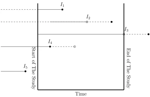
Like censoring, we have random and fixed left or right truncation, and interval truncation. Fixed left (right) truncation occurs when only subjects whose event time is greater (smaller) than a fixed age can be observed. In random left (right) truncation, the fixed age is replaced by another positive random variable. For interval truncation, the event of interest should happen within some prespecified interval for a subject to be observable. It is then clear that fixed left and right truncations are special cases of interval truncation, where one side of the interval is ∞ or −∞, for left and right truncation respectively. Figure 2.1 illustrates some types of censoring and truncation.
2.3 Analysis of survival data
In this section we introduce some basic concepts in survival analysis.
non-St ar t of T he St ud y Time E nd of T he St ud y I1 I2 I3 I4 I5
Figure 2.1 Dashed line for each individual is the time the individual is not observed. Straight lines are the time that each individual is observed. Empty circles are the censoring time, and solid circles are the time that event of interest happened. I1 is a complete observation,
I2 is random right censoring, and I3 is type I right censored individuals. I4 is random left
truncation, and I5 is an individual who are not observed because of truncation.
negative values. In survival analysis, instead of the cumulative distribution function of T , i.e. F (t) = P (T ≤ t), we mostly use survival function, which is the probability of an indi-vidual surviving beyond time t. Survival function is denoted by S(t) = P (T > t). Another fundamental concept in survival analysis is the hazard rate function (or risk function). This function represents the instantaneous density of failure, i.e. the chance for an individual who has survived until time t, to experience the event of interest in the next instant in time. Mathematically the hazard rate function is defined by
h(t) = lim
∆t→0
P(t ≤ T < t + ∆t|T ≥ t)
∆t .
There is, of course, one-to-one correspondence between F , S(t) = (1 − F (t)) and h(t). Below we present these relationships.
S(t) = P (T ≥ t) =Z ∞
F(t) = 1 − S(t) (2.2) f(t) = −dS(t) dt (2.3) h(t) = f(t) S(t) = −dlog{S(t)} dt (2.4)
All the above formulas can be proved easily. You can refer to Klein and Moeschberger (1997). In addition to all these definitions, another quantity is the cumulative hazard function H(t), defined by:
H(t) =Z t
0 h(x)dx = − ln{S(t)}. (2.5)
Thus, we can have the following formula for continuous lifetime variable:
S(t) = exp{−H(t)} = exp{−Z t
0 h(x)dx} (2.6)
One aim of survival analysis is to fit a model, for any of the above three functions, on a dataset. There are several ways to fit a model to data. Constructing the likelihood function is one of the useful methods which helps us to fit parametric or non-parametric models on a dataset. In the next section we illustrate how to construct the likelihood function for survival datasets.
2.3.1 Likelihood construction
While constructing the likelihood function, it is necessary to take in to account censored and truncated individuals. Whether an observation is censored, truncated, or an exact lifetime, it will have a different effect on the likelihood estimation.
When the event has happened for an individual, the probability of occurrence of the event at the time of happening is taken into account. Therefore, the probability density function at the time of occurrence of the event of interest is integrated into the likelihood function. When a right-censored observation exists, the probability of the individual survived past the censoring time is taken into account in the likelihood function. This probability can be approximated by the survival function evaluated at the censoring time. When a left-censored observation occurs, it means the event has already taken place, and corresponding cumulative density function evaluated at the censoring time contributes in the likelihood function. For an interval-censored observation, it is known that event occurred inside an interval, and
hence the probability of the event occurred during this interval (this can be calculated by using either S(t) or F (t)) is added to the likelihood function. Confront with truncated data means we should use a conditional probability function, because observed individuals are those individuals who experience the event of interest within a certain time interval. For example, having right-truncated data means the information, required for likelihood function, is provided by chance of experiencing the event of interest at certain time conditional on not surviving before the end of follow-up.
The likelihood function, L(θ), for a data set is constructed by taking the product of each individual component. For example, consider a dataset that consists of the observed lifetimes and right-censored observations. The likelihood for this data set in the case of independent censoring and truncations is:
L(θ) ∝ Y i∈D fθ(xi) Y i∈R Sθ(xi), (2.7)
where D and R represent the set of observed lifetimes and right-censoring times respectively, and xi is the observed lifetime for ith individual, and θ is the statistical parameters.
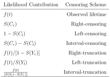
The following table shows the information components that we can use for every censoring scheme to construct likelihood function, see Klein and Moeschberger (1997).
Table 2.1 Censoring schemes and the Likelihood Function. Yl and Yr are the left and right
boundaries of follow-up time for truncated data. Cr and Cl are right and left censoring times
for censored individuals.
Likelihood Contribution Censoring Scheme
f(t) Observed lifetime S(Cr) Right-censoring 1 − S(Cl) Left-censoring S(Cr) − S(Cl) Interval-censoring f(t)/[1 − S(Yr)] Right-truncation f(t)/S(Yl) Left-truncation f (t)
2.4 Survival models
Analysing survival data requires to estimate the basic functions related to the data, like survival function or hazard rate function. This estimation is possible through parametric, nonparametric or semiparametric methods. Here, we introduce these methods briefly. Different types of censoring lead to the different likelihood function. To avoid complexity and redundant discussion, the concept of censored observation is limited to the right cen-sored observations in this study. The other types of censoring have equivalent models and inferences. During the current study, it has been considered that dataset includes typical right censored individuals who are identified by the pair (xi, δi), in which xi is the observed
time, and δi is a Bernoulli indicator with value 1 for uncensored individuals and value 0 for
censored individuals.
2.4.1 Nonparametric survival models
To draw an inference about the distribution of some time to event variable, based on a sample of right-censored dataset, Kaplan and Meier estimator (KME) is a replacement for empir-ical distribution function for ordinary data. KME is a nonparametric estimation method; Klein and Moeschberger (1997).
Kaplan-Meier estimator
Suppose Yi provides the number of individuals who are at risk at time xi. In other words, Yi
is the number of individuals who are alive and have not yet been censored up to time xi or
have observed time equal to xi. Again, assume Ei is the number of individuals who
experi-ence the event of interest at time xi. Therefore, the conditional probability that an individual
who survives just prior to time xi experiences the event of interest at time xi is equal to Ei/Yi.
The Product-Limit estimator proposed by Kaplan and Meier, in order to non-parametrically estimate the proportion of the population whose lifetimes surpass time t, is defined by
ˆ S(t) = Y xi≤t {1 − Ei Yi }. (2.8)
is not well defined when t is greater than the largest observed survival time. The variance of KME is estimated by
ˆ V { ˆS(t)} = ˆS(t)2 X xi≤t Ei Yi(Yi− Ei) . (2.9)
2.4.2 Parametric survival models
Parametric survival models have been used widely to analyze survival data. Parametric sur-vival models fit a parametric sursur-vival function to a dataset. Then it is necessary to learn more about the standard parametric survival functions, and other related functions that have been introduced in Section 2.3.
In this section, we present briefly three parametric functions in survival analysis which have frequently been used in analyzing such data. Exponential, Weibull, and lognormal are three parametric functions we will discuss among all other models such as gamma, loglogistic, nor-mal, exponential power law, and so on.
Exponential
This model suggests the density function for survival data with exponential distribution. Using equations (2.1) to (2.6), we can easily obtain other related functions of exponential survival model.
f(t) = λ exp(−λt), λ >0, t ≥ 0 (2.10)
S(t) = exp(−λt), (2.11)
h(t) = λ. (2.12)
Because of the well-known feature of exponential distribution which is lack of memory or memoryless property, we cannot fit this model for many real types of survival data. Because this property provides E(T ) = 1/λ, that means, the mean residual life time is constant which does not apply for many types of real data. We can see that exponential hazard function is also constant, which adds another restriction in applying this model for real survival datasets.
Weibull
Weibull distribution is being used commonly in survival analysis. With Weibull distribution, we can bypass the restrictions of using exponential distribution, and have more freedom in fit-ting different kinds of real datasets. The exponential distribution is a special case of Weibull distribution. The related functions and parameters with this survival model are given below:
f(t) = αλtα−1exp(−λtα), α, λ >0, t ≥0 (2.13)
S(t) = exp(−λtα), (2.14)
h(t) = αλt(α−1), (2.15)
where α is the shape parameter and λ is the scale parameter. This model has more flexibility to fit on real survival datasets. Because the hazard function of Weibull survival model can take any form of increasing, decreasing or constant for different values of α, and λ.
Lognormal
A random variable T is said to follow the lognormal distribution if its logarithm (Y = ln T ) follows the normal distribution. This distribution has been widely used for time to event datasets because of its relation to the normal distribution. We can specify this model by two parameters, the location (µ), and the scale (σ) of Y . The following equations describe the parameters of this model explicitly:
f(t) = exp[−1/2{ ln(t)−µ σ } 2] t(2π)1/2σ , σ >0, t ≥ 0 (2.16) S(t) = 1 − Φ{ln(t) − µ σ }, (2.17)
where Φ(x) is the cumulative distribution function of a standard normal variable. The hazard ratio function can be obtained by the f (t)
S(t) formula.
This survival model is very popular in applied survival analysis, because of its link to the normal distribution function which is very powerful in modeling natural phenomenon.
Accelerated failure time (AFT) model
So far, all the survival models that we have introduced are univariate survival models. But, In many cases, we are interested in figuring out how some factors can affect the surviving time. The factors are usually called covariates in the statistical literature. In other words, the event time, T > 0 could be associated with a vector of explanatory covariates, z⊤= (z
1, z2, ..., zp).
The z⊤ may include quantitative or qualitative covariates or time-dependent covariates. In
this case, we are interested in ascertaining the relationship between time to failure variable T , and the covariates z⊤. This would be the case when we want to compare survival functions
for more than one treatment, or controlling of the confounders.
One approach to the modeling of covariate effects is to use classical linear regression. In this approach, the natural logarithm of the time to event variable is denoted Y = ln(T ). This transformation is used in order to convert positive variables to observations on the entire real line. The linear model for Y is:
Y = β0+ z⊤β+ ε, (2.18)
where β is a vector of regression coefficients, β0 is a constant, and ε is a random error.
Each error distribution yields a specific model for survival time. For example, if the error distribution is the standard normal distribution, the survival time has lognormal regression model. If the error distribution is the logistic distribution, survival time has the log-logistic model, and the extreme value error distribution gives Weibull regression model. To know more about error distributions, the reader can refer to Klein and Moeschberger (1997). This method of modelling is called accelerated failure time model. We can find coefficients and unknown parameters of the specific parametric model that we are using, by constructing and maximizing a likelihood function.
2.4.3 Semiparametric survival models
Semiparametric models combine a parametric model for some components of the model and keep nonparametric estimation for other components. The following sections describe some of the semi-parametric methods in survival analysis.
Modeling with hazard rate function
Although the modelling of the time to failure provides a very useful framework for a consider-able number of cases in the real application, its use is restricted by the error distributions that one considers. Conditional hazard rate as a function of the covariates is the major method for modelling the effects of covariates on survival data. Two popular models are used for this reason, one is the multiplicative hazard model, and the other one is the additive hazard rate model. The following paragraphs describe these two approaches briefly.
Multiplicative hazard rate models: Consider for instance that we want to compare the survival function of cancer patients on two different treatments. One form of a regression model for the hazard function that could be used in such a model is:
h(t, z, β) = h0(t)r(z, β), (2.19)
in which the h0(t) could have any arbitrary parametric form or it can be any nonnegative
function of t, and r(z, β) is a nonnegative function of covariates which does not depend on t. This model could contain both parametric and nonparametric factors. These factors must be chosen so that h(t, z, β) > 0. The function h0(t) is called the baseline hazard function,
the hazard function for the subjects with covariates set to zero. It is equal to the hazard function when r(z, β) = 1. The ratio of model (2.19), for two individuals with covariate values denoted by z1, and z2, is:
HR(t, z1,z2) = h(t, z1, β) h(t, z2, β) = h0(t)r(z1, β) h0(t)r(z2, β) = r(z1, β) r(z2, β) . (2.20)
It can be seen that the hazard ratio (HR) depends only on the function r(z, β). The impor-tant part of estimation for this regression model is to determine a parametric form for r(z, β).
Cox (1972), one of the leaders in survival analysis, proposes the model (2.20). He suggested the function ez⊤β as a replacement for function r(z, β). In this case the hazard ratio (HR) is
equal to:
HR(t, z1,z2) = e(z1−z2)
⊤β
If we use the equation (2.6), the survival function for this model has the following form:
S(t, z, β) = e−H(t,z,β). (2.22)
To obtain H(t, z, β), which is the cumulative hazard function at time t for a subject with co-variate z, we can use the following method. Here, we assume the survival time is continuous. For more information refer to Cox (1972).
H(t, z, β) =Z t
0 h(u, z, β)du = r(z, β) Z t
0 h0(u)du = r(z, β)H0(t), (2.23)
in which H0(t) is called the cumulative baseline risk. Thus it follows that
S(t, z, β) = [e−H0(t)]r(z,β)= {S
0(t)}r(z,β), (2.24)
where, S0(t) = e−H0(t) is the base line survival function. So, under the Cox model the survival
function is equal to
S(t, z, β) = {S0(t)}exp(z
⊤β)
. (2.25)
Cox proportional hazard model (CPH) is useful when we want to compare two or more groups of survival data, because by applying equation (2.20), there is no need to specify the base line hazard function in the analysis of such datasets.
Additive hazard rate models: Consider we have an event time T whose distribution depends on a vector of possibly time-dependent covariates, z⊤(t) = (z
1(t), ..., zp(t)). We
assume that the hazard rate at time t, for each individual, is a linear combination of the zk(t)′s: h(t|z(t)) = β0(t) + p X k=1 βk(t)zk(t), (2.26)
The p regression functions can be positive or negative, but the values are constrained because h(t|z(t)) must be positive. Estimation for additive models is typically made by nonparamet-ric (weighted) least-squares methods; see Klein and Moeschberger (1997) for more details.
Linear transformation models
A generalization of semi-parametric models proposed above is the linear transformation model which has the form:
where z is a vector of covariates and ε is a random error with distribution function F , and β is a vector of coefficients. Another equivalent form of the linear transformation model is defined by:
g{S(t|z)} = h(t) + z⊤β, (2.28)
in which h(t) is a completely unspecified strictly increasing function, and g(t) is a known decreasing function such that g−1(t) = {1 − F (t)}. By specifying the distribution of ε, F (t),
or specifying g(t) we can precisely determine the transformation model of equation (2.27). If we consider F to be the extreme value distribution, F (x) = 1−exp{− exp(x)}, then equation (2.27) has the form of proportional hazard model, since g(x) = log(− log(x)), and equation (2.28) will convert to:
log[− log{S(t|z)}] = h(t) + z⊤β, (2.29)
which (this form) is equivalent to equation (2.25), the CPH model. The advantage of lin-ear transformation model is its generality, since F could be any distribution function. The reader can find the estimating equations of β in Cheng et al. (1995). The consistency and asymptotic normality of the estimate of β has been proven in this article.
CHAPTER 3 CURE RATE MODELS: CLASSICAL APPROACH
3.1 Introduction
Cure rate models are a special case of survival models where a portion of subjects in the population never experience the event of interest. Such subjects are called immune or cured. There are two platforms for cure models i) the mixture cure rate models, also known as standard cure rate models, which have been widely used for modelling survival data with a cured fraction. ii) the non-mixture cure rate models which have attracted less attention so far.
The survival time of cured individuals might be censored at the end of the follow-up study. Hence, if the follow-up time is long enough, there might be cured individuals in the dataset. In general, however, cured individuals comprise a subset of censored individuals. The chal-lenging aspect of fitting cure models on survival data is that the presence of cured fraction in the sample is not obvious. It is recommended to test the existence of an immune fraction in the sample before fitting cure models, and also test whether the follow-up is long enough or not. In this chapter some preliminary tests are first introduced. We then present parametric and non-parametric mixture cure models.
3.2 Preliminaries
One main reference for the materials in this section is Maller and Zhou (1996).
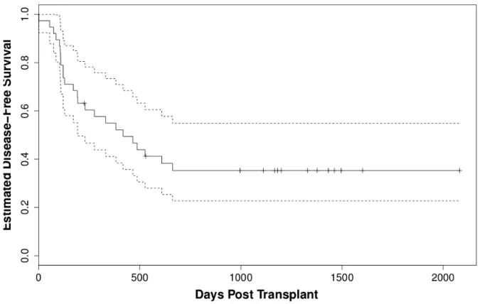
Farewell (1986) illustrates some restrictions that one confronts when applying cure models, in particular, the mixture models. One restriction is that one needs strong scientific evidence for the existence of two or more substructures in the population when applying mixture models on a dataset. It is reasonable to think that cure models in a clinical setting are sensible only if the data are based on a long-term follow-up study. The use of such models therefore requires careful attention. Visually, the presence of cured fraction in the dataset can be seen when the Kaplan-Meier survival curve reach a plateau, see in Figure 3.1. A test statistics to verify the presence of a cured fraction is proposed below.
Let T with cumulative distribution function F , and C with cumulative distribution function G, respectively, represent the failure and censoring time. Suppose δ is the censoring indicator,
Figure 3.1 Kaplan-Meier estimator for group 1 of patients in bone marrow transplant data. Doted lines are a confidence interval.
i.e. δ = 1 if T ≤ C, and 0 otherwise. Then the observations are D = {(xi, δi), i = 1, 2 . . . , n}
where xi = min(ti, ci), i = 1, 2, . . . , n and n is the sample size.
In general a cumulative distribution function A is a proper distribution function if 1. A(∞) = limt→∞A(t) = 1,
2. A(−∞) = 0.
The distribution function A(t) is improper if one of the above conditions does not apply. In mixture cure rate formulations G(t), the distribution function of censoring times, is required to be proper, but F (t), the distribution function of the event times, is not required to be a proper cumulative distribution function; Maller and Zhou (1996, p. 31).
Suppose
p= P (T < ∞) = F (∞) = lim
t→∞F(t). (3.1)
The probability p is the proportion of individuals in the population who eventually experience the failure, or the event of interest, if the follow-up time is long enough. This probability p which is always less than or equal to 1, sometimes can be strictly less than 1. Therefore, the immune fraction of population is 1 − p, i.e. the proportion of individuals in the population
who never experience the event of interest. From equation (3.1) it can be seen that F (t) could be an improper distribution function.
Let
τA= inf{t ≥ 0 : A(t) = 1}; (3.2)
The τAis called the right extreme of the distribution A(t). If the function F (t) is an improper
distribution function τF is ∞, since F (t) ≤ F (∞) < 1, for all t.
In Section 3.2.1, we highlight some questions that should be addressed prior to analysing time-to-event data.
3.2.1 Determination of cured fraction
Assume that τG < τF. This assumption is crucial for identifiability in nonparametric and
semi-parametric settings, but can be relaxed in parametric settings.
From equation (3.1) it is concluded that immune subjects are present in the population if and only if
p= F (∞) < 1.
Since, if F (∞) = 1 there is no immune fraction. Given that it is impossible to calculate F (∞) when F (t) is unknown, we consider F (τG) as the base for developing a test of hypothesis, as
it is suggested in Maller and Zhou (1996, p. 36).
We therefore consider H01: F (τG) = 1 to test for the presence of immune fraction. If H01 is
accepted, there is no evidence of having an immune fraction. If H01 is rejected, we test for
having a long enough follow-up.
To obtain a value for τG, it is needed to know the distribution of the censoring time, G. In
most practical applications, however, G is unknown as well. Therefore, the largest observed time in the sample is used instead of τG. Suppose x(n) is the largest observation, censored or
uncensored, in the sample, and ˆFn{x(n)} is the value of Kaplan-Meier estimator at x(n). A
nonparametric estimator of p is
ˆ
pn= ˆFn{x(n)}. (3.3)
It has been proved that ˆFn{x(n)} is a consistent estimator for F (τG) under a mild continuity
condition and τG ≤ τF; see Maller and Zhou (1996, chap. 3). Since ˆFn{x(n)} is an estimate
for F (τG), if ˆpn= 1, H01 is accepted and there is no immune fraction in the population. To
Reject H01 if ˆpn < cα, (3.4)
where cαis the αthpercentile of the distribution of ˆpnunder H01. To obtain the value of cα, the
distribution of ˆpnis needed, and in general this distribution is unknown; see Maller and Zhou
(1996) 1 who performed simulations to estimate the value of c
α, when α is equal to 1%, 5%,
10%, or 20%.
3.2.2 Is the follow-up time long enough?
Observations in a sample may consist of two different groups, the cured individuals (we some-times refer to them as insusceptible or immune individuals), and the uncured (we somesome-times refer to them as susceptible or nonimmune). Note that susceptible individuals could be either censored or not censored, i.e. those individuals whose event time is observed during the study period are not censored.
Suppose
F∗(t) = F(t) F(∞).
The function F∗(t) is the proper distribution function of susceptible individuals, i.e.
F∗(∞) = F(∞) p = 1.
Analogously, τF∗ is the extreme value of the survival times of susceptible individuals.
When τF ≤ τG, we may observe the largest possible event time up to the maximum possible.
In contrast, when τF > τG, it means censoring is so heavy and we may not be able to observe
all event times.Therefore, τF ≤ τG can be used to examine whether the follow-up time is
enough. Note that for susceptible individuals if ti ≤ ci then the failure time for individual
ith is observed. It is straightforward that τ
F∗ < τF. In Maller and Zhou (1996) τF∗ ≤ τG is considered as the reference for enough follow-up time. For more details see Maller and Zhou (1996, p. 33).
Therefore the desired hypothesis test for sufficient follow-up time is H02 : τF∗ ≤ τG Hc 02 : τF∗ > τG. (3.5)
This means only the magnitude of τG − τF∗ needs to be estimated, the distance between largest possible censored time and largest possible failure time of susceptible individuals. Assume x(n) is the largest observed survival time; and t(n) is the largest uncensored failure
time, it has been proved that
x(n)− t(n)→ τG− τF∗ if τG ≤ τF∗ 0 if τG > τF∗, almost surely as n → ∞ (Maller and Zhou (1996)).
Consequently, long enough follow-up time is the result of two conditions:
i) whether the presence of immune fraction is accepted in the sample, i.e. H01 is rejected.
ii) if x(n)− t(n) is large enough.
Then one can accept that the follow-up is sufficient. However, since the distribution of x(n)− t(n) is unknown, a simpler quantity should be found to perform this hypothesis test.
To this end Maller and Zhou (1996) defined
qn =
Nn
n =
Number of uncensored xi in the interval (2t(n)− x(n), t(n)]
Number of sample individuals (3.6)
to test this hypothesis.
Large values of qnsuggest rejecting Hc02or equivalently accepting H02. This means the
follow-up time is long enough. However, how large qn must be to accept H02 is still unclear, since
the distribution of qn(and Nn) is unknown. Again the simulation results of Maller and Zhou
(1996) can be used to evaluate the percentiles of distribution of qn. If the value of qn
3.3 Mixture cure rate models
Most of the early works in cure rate models are based on parametric mixture models. In this section we aim to explain one of the earliest work in mixture cure rate models. Some other parametric, nonparametric, and semi-parametric methods are discussed in sections 3.4, 3.5, and Chapter 4. We start with a simple parametric version of mixture cure rate model, using the exponential distribution function for the survival time.
3.3.1 History
The paper by Berkson and Gage (1952) is our main reference in this section. The idea of mixture cure rate models originates from comparison between survival curves of two groups of subjects. One group is the patients under a specific treatment, and the other is a sample from a control group. Consider logarithm of survival times in drawing two survival curves and draw them on one figure. The ratio of survival times of two groups can be found by vertical difference between the two curves. It has been shown that the two curves approxi-mately become parallel after passing some time. It means the instantaneous failure rate for the two curves is equal, and failure rate for group of patients who are under the treatment becomes equal to failure rate for the controlled group, at some point. Cured fraction is the proportion of patients who are subject to normal failure rate in the controlled group. This definition of cured fraction first appeared in Berkson and Gage (1952).
Berkson and Gage (1952) divide the population in two hypothetical groups, one group is just subject to normal failure rate which is called cured fraction. The other group is subject to normal failure rate and a specific failure rate which could be the failure rate for a disease under the study. These two failure rates are represented by q0, for normal failure rate, and
qca, for the specific failure rate of the disease. These two failure rates act independently and
simultaneously. Assume the two groups act separately, then the probability of survival for the cured fraction is l0 =Qni=1(1 − q0), and the probability of survival for uncured fraction is
l0lca, in which lca =Qni=1(1 − qca).
Berkson and Gage (1952) made another assumption to simplify their modelling. They con-sidered the rate of death caused by the specific disease to be a constant (say β), i.e. the hazard function for uncured population is β. So the survival probability for the uncured population should decrease exponentially and be time-varying, implying that lca(t) = e−βt.
time t for total population is
Probability of survival up to time t = pl0+ (1 − p)l0e−βt. (3.7)
The unknown parameters in equation (3.7) are p and β. Dividing both sides of equation (3.7) by l0 we have
Probability of survival up to time t l0
= p + (1 − p)e−βt. (3.8)
The equation (3.8) can be interpreted as the probability of survival in the whole population. This interpretation is valid only if the population is free of death by any other causes, except the disease of interest. Parameters p and β are estimated by least squares method using one of the numerical minimization routines. For complete details of minimization methods see Berkson and Gage (1952).
Berkson and Gage (1952) did not consider any censorship for the data during the experi-ment. Cured individuals are those who survive by the end of the experiment, and uncured individuals are those who are faced with the event of interest during the follow-up.
3.3.2 Formulation of mixture models
In survival analysis, observations usually consist of the following random variables.
Random variable X = min{T, C}, where T is the failure time, and C is censoring time, and Bernoulli variable δ = 0 if the individual is censored, and is equal to 1 otherwise. Also, some covariates may be added to these variables. We often assume that T and C are independent.
Subjects can be divided in another category which divides individuals between susceptible (uncured) and insusceptible (cured) individuals. A Bernoulli random variable η is an indi-cator for susceptibility of each individual. This variable η takes value 1 if the individual is susceptible and 0 otherwise. Of course, η is not observed; essentially, there is no information from a study, but it has been used as a latent variable in the model formulation. To distin-guish properly the difference between variables η and δ, consider η as the true event status and δ as the observed failure status; essentially, {δi = 1, i = 1, . . . , n} ⊂ {ηi = 1, i = 1, . . . , n},
where i denotes an individual and n is sample size. The latent variable η enable us to divide event time in two categories: those individuals who meet the event, and those who never
meet the event of interest. Following the decomposition for event (failure) time:
T = ηT∗+ (1 − η)∞. (3.9)
Equation (3.9) illustrates that failure time T is decomposed by T∗, the survival time of
susceptible individuals, and survival time of insusceptible individuals which conventionally is considered to be ∞ and never happens. By introducing η the true survival time, T = ∞ becomes reasonable. We introduced before F∗(t) as the proper cumulative distribution for
survival time; thus,
P(T ≤ t|η = 1) = F∗(t), (3.10)
P(T ≤ t|η = 0) = 0. (3.11)
The density and survival functions of cured individuals are set to zero and one, respectively, for all finite values of t because cured (insusceptible) individuals will never experience the failure. Thus,
F(t) = P (T ≤ t) = P (T ≤ t|η = 1)P (η = 1) + P (T ≤ t|η = 0)P (η = 0) (3.12) = pF∗(t) + 0 = pF∗(t). (3.13)
The last equality holds since P {η = 1} = p. The overall formulation of a mixture cure rate model is derived from the above equation. Briefly, the mixture cure rate models have the form
F(t) = pF∗(t), (3.14)
or equivalently,
S(t) = (1 − p) + pS∗(t). (3.15)
The functions S(t) and S∗(t) are improper and proper cumulative survival functions of T .
Consequently, f∗(t) is a proper density function of T .
In the previous part, equation (3.7) is equivalent to the mixture formulation of equation (3.15), if T has exponential distribution with parameter β.
3.3.3 Likelihood function for mixture models
The general likelihood function for mixture rate cure model is
L(θ, p) = n Y i=1 {pfθ∗(t)}δi{pS∗ θ(t) + (1 − p)}1−δi, (3.16)
where θ is a vector of statistical parameters, and the functions S∗
θ(t) and fθ∗(t) are identified
with these parameters. To simplify notation we stop writing index θ repeatedly unless for emphasizing and remembering this.
This likelihood is derived from the fact that the probability of experiencing the event for those individuals who are not censored at time t is pf∗
θ(t), and the probability of staying
alive up to time t for those individuals who have been censored at time t is pS∗
θ(t) + (1 − p).
The specification of S∗
θ(t), or equivalently fθ∗(t), can be parametric or nonparametric, which
leads to parametric and nonparametric mixture models.
3.4 Parametric mixture models
Parametric mixture cure rate models are obtained by simply considering a parametric model for S∗
θ(t) in equation (3.15). The most frequently used parametric models for Sθ∗(t) are
Weibull, logistic, and exponential.
3.4.1 Weibull and conditional logistic mixture model
The susceptibility variable, η, has been defined by ?. He divides individuals into two cohorts, one cohort is those individuals who face by the event of interest during the follow-up, η = 1, and another is those individuals who survive by the end of experiment, and these could have either η = 0 or η = 1.
The term π(γ⊤w) has been used here as the cured fraction, p in equation (3.15) to
empha-size the dependency of cured fraction on some covariates, w. Obviously γ is the vector of related covariate coefficients to be estimated. To connect the cure fraction with the vector of covariates, a link function is needed. Logistic regression is an option for link function as follows:
P(η = 1|w) = π(γ⊤w) = exp(γ
⊤w)
1 + exp(γ⊤w). (3.17)
Also, to emphasize the possibility of a connection between survival time of individuals and some covariates like vector z, the mixture model formulation which is introduced by equation (3.15) can be reformulated with the following notation:
S(t|w, z) = 1 − π(γ⊤w) + π(γ⊤w)S∗(t|z). (3.18)
In the above equation for time to event variable, T , two different parametric models have been assumed, one for individuals who are susceptible and the other one for those who are not susceptible. Consider the probability of survival for susceptible individuals (η = 1), with covariate vector z, is obtained by Weibull distribution, Farewell (1982). The Weibull distri-bution function is defined in (2.13), where λ = exp(−β⊤z) is replaced with scale parameters,
and vector β represents unknown regression coefficients. Note that the parameter λ differs for each individual because of covariate the vector z.
We refer to the combination of (3.17) and Weibull distribution function as Weibull mixture cure rate model.
Assume that no individual with η = 0 experience failure during the follow-up. The unknown parameters are estimated using maximum likelihood. The probability of failure at time t for an individual is P (η = 1|z)f(t|η = 1, z). If the individual has been followed completely during the study, the probability of survival by the time t becomes
{1 − P (η = 1|z)} + P (η = 1|z)Z ∞
t f
∗(s|η = 1, z)ds. (3.19)
The likelihood function has the form of equation (3.16), where S∗(t) = R∞
t f∗(s|η = 1, z)ds,
and f∗(t) is replaced by Weibull distribution function. The cured fraction, p, also is
re-placed by parametric model of equation (3.17). An iterative method, like Newton-Raphson, is adopted to maximize the log likelihood function, numerically.
3.5 Nonparametric mixture models
In this section a nonparametric estimation is assumed for F∗, the cumulative distribution
of the survival times for susceptible individuals. The first nonparametric model that crosses the mind to fit on survival data is Kaplan-Meier estimator. In statistical modelling context usually the aim is to examine the effects of multiple covariates on the response variable. In
cure rate models, one of the goals is to investigate how other factors can affect the cured fraction and the survival time of susceptible patients. Cox proportional hazard (CPH) model is a well-known survival model to investigate the effect of covariates on survival time. The following section aims to explain a nonparametric approach for mixture cure rate models, using CPH model.
3.5.1 Proportional hazard mixture model
The material of this section is acquired from Peng and Dear (2000). To study a general nonparametric mixture model, the CPH model can be a good choice for connecting failure time to some covariates. Because CPH model is specifically appropriate for survival data and relaxes the normality assumption. The EM algorithm is another tool that has been used for estimating parameters in this method Dempster et al. (1977).
Again, suppose that z and w are two covariate vectors related to each individual, in which the distribution of T∗, and cured fraction, respectively, may depend on them.
For susceptibility indicator a model similar to equation (3.17) can be considered, and S∗(t|z)
is replaced with survival CPH function to model the effects of covariate z on the failure distribution of susceptible individuals. The CPH model takes the following form:
h∗(t|z) = h∗0(t) exp(z⊤β), (3.20) in which h∗(t) is hazard function, and h∗
0(t) is the baseline hazard function and can be any
ar-bitrary specified hazard function but not a function of z. This leads to S∗(t|Z) = S∗
0(t)exp(β
⊤
z)
as a model for survival function of susceptible individuals, where S∗
0(t) = exp{− Rt
0h∗0(s)ds}.
EM algorithm can be used to estimate γ in (3.17), and β in (3.20).
EM algorithm is an iterative method for finding locally maximum likelihood and for estimat-ing parameters in a model. This algorithm has been applied usually when it is assumed there are some unmeasured parameters in the dataset. These unmeasured parameters is sometimes called missing values. This method consists of two steps, the E-step and the M-step. In the E-step the aim is to find expectation of complete log-likelihood (as a function of missing value) conditional on the observed values and estimated parameters in the previous itera-tion, and in the M-step the goal is to find a new estimation for the parameters of the model by maximization of the expectation of complete log-likelihood. For complete details of EM