Magnetospherically reflected chorus waves revealed by ray tracing with CLUSTER data

(1)

HAL Id: hal-00329252

https://hal.archives-ouvertes.fr/hal-00329252

Submitted on 1 Jan 2003

HAL is a multi-disciplinary open access

archive for the deposit and dissemination of

sci-entific research documents, whether they are

pub-lished or not. The documents may come from

teaching and research institutions in France or

abroad, or from public or private research centers.

L’archive ouverte pluridisciplinaire HAL, est

destinée au dépôt et à la diffusion de documents

scientifiques de niveau recherche, publiés ou non,

émanant des établissements d’enseignement et de

recherche français ou étrangers, des laboratoires

publics ou privés.

ray tracing with CLUSTER data

Michel Parrot, O. Santolik, N. Cornilleau-Wehrlin, M. Maksimovic, C. Harvey

To cite this version:

Michel Parrot, O. Santolik, N. Cornilleau-Wehrlin, M. Maksimovic, C. Harvey. Magnetospherically

reflected chorus waves revealed by ray tracing with CLUSTER data. Annales Geophysicae, European

Geosciences Union, 2003, 21 (5), pp.1111-1120. �hal-00329252�

(2)

Annales Geophysicae (2003) 21: 1111–1120 c European Geosciences Union 2003

Annales

Geophysicae

Magnetospherically reflected chorus waves revealed by ray tracing

with CLUSTER data

M. Parrot1, O. Santol´ık2, N. Cornilleau-Wehrlin3, M. Maksimovic4, and C. Harvey5

1_{LPCE/CNRS, 3A Avenue de la Recherche, ORLEANS, 45071 France}

2_{Charles University, V. Holesovickach, Praha, 18000 Czech Republic}

3_{CETP/UVSQ, 10/12 Avenue de L’Europe, Velizy, 78140 France}

4_{LESIA, place Jules Janssen, Meudon, 92195 France}

5_{CESR, 9 Av. Colonel Roche, Toulouse, 31029 France}

Received: 29 October 2002 – Revised: 20 February 2003 – Accepted: 4 March 2003

Abstract. This paper is related to the propagation character-istics of a chorus emission recorded simultaneously by the 4 satellites of the CLUSTER mission on 29 October 2001 be-tween 01:00 and 05:00 UT. During this day, the spacecraft (SC) 1, 2, and 4 are relatively close to each other but SC3 has been delayed by half an hour. We use the data recorded aboard CLUSTER by the STAFF spectrum analyser. This instrument provides the cross spectral matrix of three mag-netic and two electric field components. Dedicated software processes this spectral matrix in order to determine the wave normal directions relative to the Earth’s magnetic field. This calculation is done for the 4 satellites at different times and different frequencies and allows us to check the directions of these waves. Measurements around the magnetic equa-tor show that the parallel component of the Poynting vecequa-tor changes its sign when the satellites cross the equator region. It indicates that the chorus waves propagate away from this region which is considered as the source area of these emis-sions. This is valid for the most intense waves observed on the magnetic and electric power spectrograms. But it is also observed on SC1, SC2, and SC4 that lower intensity waves propagate toward the equator simultaneously with the SC3 intense chorus waves propagating away from the equator. Both waves are at the same frequency. Using the wave nor-mal directions of these waves, a ray tracing study shows that the waves observed by SC1, SC2, and SC4 cross the equato-rial plane at the same location as the waves observed by SC3. SC3 which is 30 minutes late observes the waves that origi-nate first from the equator; meanwhile, SC1, SC2, and SC4 observe the same waves that have suffered a Lower Hybrid Resonance (LHR) reflection at low altitudes (based on the ray tracing analysis) and now return to the equator at a dif-ferent location with a lower intensity. Similar phenomenon is observed when all SC are on the other side of the equator. The intensity ratio between magnetic waves coming directly from the equator and waves returning to the equator is

be-Correspondence to: M. Parrot

(mparrot@cnrs-orleans.fr)

tween 0.005 and 0.01, which is in agreement with previously published theoretical calculation of the growth rates with the particle distribution seen by GEOS.

Key words. Magnetospheric physics (plasma waves and in-stabilities) – Ionosphere (wave propagation) – Radio science (magnetospheric physics)

1 Introduction

Chorus waves are one of the most intense emissions observed in the outer magnetosphere. They are detected near the equa-torial plane and they are characterised by a sequence of dis-crete elements (rising and falling tones) with a time separa-tion between 0.1 and 1 s. They have been extensively studied in the past (see the review by Sazhin and Hayakawa (1992) and the references herein). They are generated by the injec-tion of substorm electrons (Tsurutani and Smith, 1974; Tsu-rutani et al., 1979; Meredith et al., 2001) through the loss cone instability (Kennel and Petschek, 1966). It has been indirectly shown (Dunkel and Helliwell, 1969; Burtis and Helliwell, 1969; Burton and Holzer, 1974; Tsurutani and Smith, 1977) that the chorus emissions are generated near the magnetic equator. More recently, this was confirmed by Nagano et al. (1996) using GEOTAIL data and by LeDocq et al. (1998) with POLAR data. Parrot et al. (2003) have shown that in fact, during moderate magnetic activity, the source of the emissions is located at the magnetic equator when this equator is determined by the minimum of the in situ measured magnetic field (the SC velocity being paral-lel to this magnetic field). Around the magnetic equator, the frequency spectrum of chorus often shows that chorus have two distinct bands above and below one-half the electron gy-rofrequency (Tsurutani and Smith, 1974). Up to now all ob-servations have failed to find reflected chorus components returning to the equator. LeDocq et al. (1998) indicates that there is little evidence of reflected waves returning along the same field lines. Burton and Holzer (1974) and Goldstein and

(3)

Tsurutani (1984) claim that the chorus emissions must en-counter strong Landau damping as they propagate to high lat-itudes. The purpose of this paper is to analyse a chorus event where reflected components are observed using the wave ex-periment STAFF (Spatio-Temporal Analysis of Field Fluctu-ations) of the 4 CLUSTER satellites. STAFF will be shortly described in Sect. 2. Section 3 will present the dedicated software PRASSADCO (PRopagation Analysis of STAFF-SA Data with COherency tests) used to determine propaga-tion characteristics of the observed chorus waves, and the ray tracing program used to emulate the back and forth trajecto-ries of the waves in the magnetosphere. The chorus event simultaneously recorded by the four CLUSTER satellites is described in Sect. 4 with the results of the ray tracing analy-sis. Discussions and conclusion are given in Sect. 5.

2 The wave experiment

The STAFF experiment (Cornilleau-Wehrlin et al., 1997, 2000, 2003) is a part of the Wave Experiment Consortium (WEC) (Pedersen et al., 1997) on board the four CLUS-TER satellites. STAFF consists of three orthogonal magnetic search coils linked to a processing unit. Two sensors lie in the spin plane and the third one is parallel to the SC spin axis. The processing unit has two parts: STAFF-SC which records waveforms of the three components of the magnetic field up to 10 Hz (180 Hz in the burst mode), and STAFF-SA which computes the spectral matrix of five components of the electromagnetic field up to 4 kHz. The two electric compo-nents are from the Electric Field and Wave experiment EFW (Gustafsson et al., 2001). The SA (Spectrum Analyser) part will be used in the following. It produces 5 × 5 spectral ma-trix with 27 frequencies distributed logarithmically between 8 Hz and 4 kHz. This frequency range is divided into three frequency sub-bands: A (8–64 Hz), B (64–512 Hz), and C (512–4000 Hz) with different time intervals of Fourier anal-ysis (for example, for one second of data, 64 spectra are av-eraged in the band C, 8 in the band B, and only one spectrum is considered in band A). After averaging, the time resolution of the spectral matrix varies between 125 ms and 4 s.

3 The data processing software

PRASSADCO is a computer program designed to analyse multicomponent measurements of electromagnetic waves. It implements a number of methods used to estimate polarisa-tion and propagapolarisa-tion parameters, such as the degree of polar-isation, sense of elliptic polarisation and axes of polarisation ellipse, the wave vector direction, the Poynting vector, and the refractive index (Santol´ık and Parrot, 1998, 1999; San-tol´ık, 2001). The main purpose of PRASSADCO is to facili-tate scientific analysis of the spectral matrix obtained by the STAFF-SA instruments on board the four satellites. The in-puts of this software are the CLUSTER data CD-ROMs pro-vided by ESA, the CSDS (CLUSTER Science Data System) Prime Parameters (PP) of FGM (Flux Gate Magnetometer)

for the local magnetic field (Balogh et al., 1997), and the CSDS Summary Parameters of auxiliary data (Daly, 2002). The results can be represented in different visual and numer-ical formats. The calculation of the wave normal directions relative to the Earth’s magnetic field is done for the 4 satel-lites at different times and different frequencies according to the event we are looking at.

All these wave normal directions (two angles) obtained at a given frequency during the considered time interval are the inputs of a ray tracing program used to trace back all rays to the source. We use the three-dimensional procedure of Cerisier (1970) which was more recently used by Cairo and Lefeuvre (1986) and Muto and Hayakawa (1987). The ray tracing software uses a dipolar approximation of the mag-netic field and a diffusive equilibrium model for ion and elec-tron densities. The model is roughly calibrated at the satellite altitude by plasma parameters obtained by the WHISPER ex-periment (D´ecr´eau et al., 2001). Ray plots are represented in 3-D using a GSM (Geocentric Solar Magnetospheric) sys-tem.

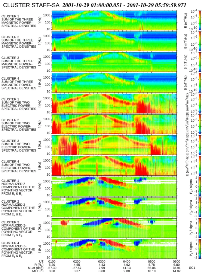
4 Detailed analysis of the event recorded by CLUSTER Figure 1 represents data recorded by the 4 spacecraft on 29 October 2001 between 01:00 and 06:00 UT. This event oc-curs during a period of moderate magnetic activity (DST is equal to −65 nT at 03:00 UT) just after a disturbed pe-riod. The first four panels show the magnetic power-spectral densities, for SC1, SC2, SC3, and SC4, respectively. The second four panels show the electric power-spectral densi-ties, for SC1, SC2, SC3, and SC4, respectively. The plot-ted spectrograms are obtained from the arithmetic average of the power-spectral densities of the three magnetic compo-nents in the first four panels, and of the two electric com-ponents in the second four panels (the power-spectral den-sities themselves being already averaged (see Sect. 2)). A banded electromagnetic emission of chorus type is seen be-tween 100 Hz and 4 kHz, with the maximum frequency being obtained when the satellite is near the magnetic equator. It has been shown by Dunkel and Helliwell (1969) and Burtis and Helliwell (1969) that the chorus emission frequency is related to the equatorial cyclotron frequency of the magnetic field line passing through the observing point. This explains why, in Fig. 1, the frequency of the chorus bands decreases on each side of the equator. In this event, chorus are ob-served below one-half the electron gyrofrequency. Besides the chorus emissions, on the one hand, turbulent electrostatic noise at low frequencies are observed in the auroral zones and close to the equator, and on the other hand, auroral hiss between 700 Hz and 4 kHz are observed in the auroral zones. But these three emissions are not related to our study and they will not be considered here. The thin vertical white lines in the electric spectrograms are due to changes in the WEC experiment mode which temporarily inhibit the observation of natural waves during WHISPER sounding (D´ecr´eau et al., 1997).

(4)

M. Parrot et al.: Magnetospherically reflected chorus waves 1113 UT: 0100 0200 0300 0400 0500 0600 R (RE): 5.20 4.55 MLat (deg): -57.39 -27.67 MLT (h): 8.38 8.37 CLUSTER 1

SUM OF THE THREE MAGNETIC POWER-SPECTRAL DENSITIES CLUSTER 2

SUM OF THE TWO ELECTRIC POWER-SPECTRAL DENSITIES CLUSTER 2

SUM OF THE TWO ELECTRIC POWER-SPECTRAL DENSITIES CLUSTER 1 NORMALIZED Z-COMPONENT OF THE POYNTING VECTOR FROM E1 & E2 CLUSTER 2 NORMALIZED Z-COMPONENT OF THE POYNTING VECTOR FROM E1 & E2 CLUSTER 3 NORMALIZED Z-COMPONENT OF THE POYNTING VECTOR FROM E1 & E2 CLUSTER 4 NORMALIZED Z-COMPONENT OF THE POYNTING VECTOR FROM E1 & E2 4.43 7.99 8.60 4.92 41.13 9.08 5.78 66.06 10.19

CLUSTER STAFF-SA

2001-10-29 01:00:00.051 - 2001-10-29 05:59:59.971

6.80 78.91 14.02 10-10 10-8 10-6 10-4 B (nT 2/Hz) 10 100 1000 f (Hz) 10-10 10-8 10-6 10-4 B (nT 2/Hz) 10 100 1000 f (Hz) 10-10 10-8 10-6 10-4 B (nT 2/Hz) 10 100 1000 f (Hz) 10-10 10-8 10-6 10-4 B (nT 2/Hz) 10 100 1000 f (Hz) 10-9 10-7 10-5 10-3 E (mV 2/m 2/Hz) 10 100 1000 f (Hz) 10-9 10-7 10-5 10-3 E (mV 2/m 2/Hz) 10 100 1000 f (Hz) 10-9 10-7 10-5 10-3 E (mV 2/m 2/Hz) 10 100 1000 f (Hz) 10-9 10-7 10-5 10-3 E (mV 2/m 2/Hz) 10 100 1000 f (Hz) -2 -1 0 1 2 PZ / sigma 10 100 1000 f (Hz) -2 -1 0 1 2 PZ / sigma 10 100 1000 f (Hz) -2 -1 0 1 2 PZ / sigma 10 100 1000 f (Hz) -2 -1 0 1 2 PZ / sigma 10 100 1000 f (Hz) SC1

Fig. 1. Data recorded by the STAFF-SA experiment on 29 October 2001 between 01:00 and 06:00 UT. From the top to the bottom, the panels represent the magnetic power-spectral density, the electric power-spectral density, and the direction of the z-component of the Poynting vector, for each SC, respectively. The intensities of the spectrograms and the reliability of the sense of the Poynting vector (see Parrot et al., 2003) are given by the colour-coded scales on the right. The geophysical parameters at the bottom are related to SC1.

(5)

UT: 0220 0230 0240 0250 0300 0310 0320 0330 0340 0350 R (RE): MLat (deg): MLT (h): CLUSTER 1 POLAR ANGLE THETA (Means, 1972) CLUSTER 2 POLAR ANGLE THETA (Means, 1972) CLUSTER 3 POLAR ANGLE THETA (Means, 1972) CLUSTER 4 POLAR ANGLE THETA (Means, 1972) CLUSTER 1 AZIMUTHAL ANGLE PHI (Means, 1972) CLUSTER 2 AZIMUTHAL ANGLE PHI (Means, 1972) CLUSTER 3 AZIMUTHAL ANGLE PHI (Means, 1972) CLUSTER 4 AZIMUTHAL ANGLE PHI (Means, 1972) CLUSTER 1 NORMALIZED Z-COMPONENT OF THE POYNTING VECTOR FROM E1 & E2 CLUSTER 2 NORMALIZED Z-COMPONENT OF THE POYNTING VECTOR FROM E1 & E2 CLUSTER 3 NORMALIZED Z-COMPONENT OF THE POYNTING VECTOR FROM E1 & E2 CLUSTER 4 NORMALIZED Z-COMPONENT OF THE POYNTING VECTOR FROM E1 & E2 4.56 4.46 4.39 4.33 4.28 -35.33 -29.62 -23.68 -17.55 -11.27 8.28 8.31 8.35 8.40 8.45 4.26 4.26 4.27 -4.88 1.55 7.97 8.51 8.57 8.64

CLUSTER STAFF-SA

2001-10-29 02:20:00.352 - 2001-10-29 03:49:59.658

0 20 40 60 80 Theta (deg) 10 100 1000 f (Hz) 0 20 40 60 80 Theta (deg) 10 100 1000 f (Hz) 0 20 40 60 80 Theta (deg) 10 100 1000 f (Hz) 0 20 40 60 80 Theta (deg) 10 100 1000 f (Hz) -180 -90 0 90 180 Phi (deg) 10 100 1000 f (Hz) -180 -90 0 90 180 Phi (deg) 10 100 1000 f (Hz) -180 -90 0 90 180 Phi (deg) 10 100 1000 f (Hz) -180 -90 0 90 180 Phi (deg) 10 100 1000 f (Hz) -2 -1 0 1 2 PZ / sigma 10 100 1000 f (Hz) -2 -1 0 1 2 PZ / sigma 10 100 1000 f (Hz) -2 -1 0 1 2 PZ / sigma 10 100 1000 f (Hz) -2 -1 0 1 2 PZ / sigma 10 100 1000 f (Hz) ₁ ₂ ₃ ₄ SC3

Fig. 2. Zoom of the event of Fig. 1 between 02:20 and 03:50 UT. From the top to the bottom, the panels represent the polar angle θ and the azimuthal angle φ of the wave normal direction, and the direction of the z-component of the Poynting vector, for each SC, respectively. The values for the angles and the reliability of the sense of the Poynting vector are given by the colour-coded scales on the right. The geophysical parameters at the bottom are related to SC3. The vertical black lines delimit the four time intervals of detailed analysis.

(6)

M. Parrot et al.: Magnetospherically reflected chorus waves 1115

Fig. 3. The top panel represents the projection of the SC orbits in the ecliptic plane, whereas the bottom panel shows the correspond-ing azimuthal angle (longitude) as a function of time in the interval 02:19:30–03:48:30 UT. The curves are colour-coded according to each SC.

The four last panels present propagation characteristics of these emissions in frequency-time plots similar to spectro-grams with intensities colour-coded according to the scale on the right. These panels give an estimation of the sign of the parallel component of the Poynting vector relative to the

Earth’s magnetic field B0(Santol´ık et al., 2001; Parrot et al.,

2003). Geophysical parameters at the bottom of Fig. 1 are related to SC1. In the Poynting vector panels, a blue colour indicates that the wave vector is in the opposite direction of

the Earth’s magnetic field B0, i.e. directed towards the south,

whereas the red colour is related to wave vectors in the

direc-tion of B0, i.e. directed towards the north. This assumption

is valid for observations at low- and mid-latitudes, which is the case in this event where the magnetic latitude is always

less than 43◦. It is observed on all SC for the main intense

chorus emissions that the colour changes close to the equator, which indicates that the chorus waves propagate away from

CLUSTER STAFF-SA 2001-10-29 02:23:59.088 - 2001-10-29 02:35:00.880 CLUSTER 1 CLUSTER 2 CLUSTER 3 CLUSTER 4 10-10 10-9 10-8 10-7 10-6 10-5 10-4 B (nT 2/Hz) 10 100 1000 f (Hz) 10-7 10-6 10-5 10-4 10-3 E (mV 2/m 2/Hz)

Fig. 4. Power spectral densities of the magnetic (top) and electric (bottom) components during the time interval 02:24–02:35 UT. The curves are colour-coded according to each SC. The peaks at 70 and 140 Hz are interferences.

the equator. In these four last panels, it is also observed at the same time below the main emissions for each satellite, emissions at lower frequencies, which for most of the time propagate in an opposite direction. These emissions are di-rected toward the equator, and it is postulated that they are related to the main intense one. This will be demonstrated in the next paragraph using ray tracing techniques.

Figure 2 represents a zoom of Fig. 1 from 02:20 until 03:50 UT, a time interval that will be studied in more details in what follows. The last group of four panels shows again the direction of the Poynting vector for the 4 SC. The first and second group of four panels represent the polar and the azimuthal angles of the wave normal direction relative to the

Earth’s magnetic field B0 (given by the FGM PP),

respec-tively. These angles are obtained from the magnetic spectral matrix with the method of Means (1972). This method can be used for these emissions because their degree of polarisa-tion (not shown here) obtained from the eigenvalues of the spectral matrices is high enough (∼0.8), which is an indica-tion of plane waves (Lefeuvre and Parrot, 1979). Geophys-ical parameters at the bottom of Fig. 2 are related to SC3.

(7)

Four time intervals have been chosen for the inverse ray trac-ing study ustrac-ing as inputs the polar and azimuthal angles of the wave normal direction, the local electron density given by the WHISPER experiment, and the relative satellite positions which are given in Fig. 3. Figure 3a represents the projection of the SC orbits in the ecliptic (X − Y ) GSE (Geocentric So-lar Ecliptic) plane. The curves are colour-coded according to each SC and the time (02:20–03:50 UT) is going from the left to the right. Figure 3b is derived from 3a; it gives the az-imuthal angle (related to the longitude) in the ecliptic plane as a function of time. At a given time, similar angles for the SC indicate that these SC are on the same meridian line.

The first time interval is from 02:24 until 02:35 UT, and Fig. 4 represents the power spectral densities of the 3 mag-netic and the 2 electric components in the top and bottom panels, respectively. The plots which represent average val-ues over the 11-min interval, are done as a function of the fre-quency for each SC, and SC3 shows a peak centred around 456 Hz according to the intensities observed in Fig. 1 (the peaks around 70 Hz and 140 Hz are due to internal interfer-ences of the Spectrum Analyser). At the same time as the peak on SC3, power spectral density increases with much lower intensities are also observed on SC1, SC2, and SC4. Four frequencies of STAFF-SA have been selected for the ray tracing: 456, 574, 724, and 912 Hz. Those frequencies are central frequencies of the different equivalent filters. It is seen on the last four panels of Fig. 2 that these frequencies correspond to SC3 waves escaping from the equator (blue) and to waves going to the equator for SC1, SC2, and SC4 (red). But it is also observed that the frequency bandwidth of the peaks observed in Fig. 4 does not fit exactly with the frequency bandwidth of the red zone in Fig. 2, and this point will be discussed later. The peak at 2896 Hz in Fig. 4 for SC1, SC2, and SC4 corresponds to the intense waves com-ing directly from the equator, which are not studied here.

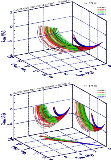
The results of the multiple ray tracing for each satellite and for each polar and azimuthal determinations of the wave normal direction between 02:24 and 02:35 UT are given in Fig. 5. Figure 5a represents the 3-D plots of the rays in GSM coordinates for 574 Hz. The ray tracing software was stopped when the rays encountered the equator. Rays corresponding to one SC are colour-coded according to the dedicated SC colours seen on the right upper corner. Each line corresponds to a ray at a different time, then trajectories of all SC between 02:24 and 02:35 UT can also be seen on this 3-D plot. They are plotted by the points of departure of each ray when the time is going on. In order to have a better view of the ray trajectories, this 3-D plot has been projected on the 3 planes

XY, XZ, and Y Z in Fig. 5b. It is clearly shown on this plot

that the waves observed, on one hand, by SC3, and, on the other hand, by SC1, SC2, and SC4, span the same region in the equatorial plane (the source region of chorus). Waves that originate from the equator are first seen by SC3. After that, they are going to higher latitudes where they suffer a LHR (Lower Hybrid Resonance) reflection at low altitudes. The reflection occurs when the frequency of the wave approaches the local LHR frequency (Kimura, 1966). At the end, they

Fig. 5. The top panel represents the ray traces in 3-D for a frequency equal to 574 Hz during the same time interval as Fig. 4. The bottom panel represents the same data but now only the projections of the ray traces on the three planes are plotted. The curves are colour-coded according to each SC.

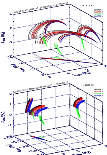
return to the equator at a different L value. On their way back, they are observed by SC1, SC2, and to a lesser extent by SC4, because a very small number of rays is obtained for this SC. Plots for other frequencies are shown in Fig. 6. They are similar to Fig. 5b and represent ray tracing for 456 and 724 Hz in Figs. 6a and 6b, respectively. At 456 Hz, it is noted that the waves observed on SC4 map in the equatorial plane to a region that is different from the other SC. This will be discussed in the next section. At 724 Hz, the results are similar to Fig. 5b, however, the extension of the source at the equator diminishes. At 912 Hz, it still decreases (not shown). The second time interval is from 02:56 until 03:05 UT and the third one is from 03:10 until 03:16 UT. SC1, SC2, and SC4 are now in the Northern Hemisphere whereas SC3 is still in the Southern Hemisphere. In the second time interval (02:56–03:05 UT), it is seen from Fig. 2 that SC1, SC2, and SC4 observe waves at frequencies between 724 and 1149 Hz going toward the equator, whereas SC3 observes the main intense emission at the same frequencies coming from the equator. In the third time interval (03:10–03:16 UT), Fig. 2

(8)

M. Parrot et al.: Magnetospherically reflected chorus waves 1117

Fig. 6. Same as the bottom panel of Fig. 5, but the top and the bottom panels correspond to 456 and 724 Hz, respectively.

indicates that SC1, SC2, SC3 and SC4 (SC3 is still in the Southern Hemisphere) observe their main emissions coming from the equator at frequencies larger than 1824 Hz. Ray plots corresponding to these second and third time intervals are shown in Figs. 7a and b, respectively. They are repre-sented on the plot in 3D together with their projections. Fig-ure 7a shows that SC1, SC2, and SC4 observe waves coming from the equator after a LHR reflection whereas SC3 observe waves coming directly from the equator. The mapping in the equatorial source region indicates that there is no relation be-tween these waves because the origin of the waves observed by SC3 does not fit with the origin of the waves observed by SC1, SC2, and SC4. However SC1, SC2, and SC4 ob-serve emissions coming from the same region. Figure 7b (time interval 03:10-03:16 UT) indicates that all SC observe their more intense emission coming directly from the equa-tor. Waves observed on the one hand by SC1, SC2, and SC4 and on the other hand by SC3 are again not coming from the same region because there is no overlap of the source regions in the X-direction. At lower frequencies, the SC3 panel of Fig. 2 (z-component of the Poynting vector) also in-dicates that different waves return to the equator during this

Fig. 7. The ray plots are represented (together with their projec-tions in the three planes) in the top and bottom panels for the time intervals 02:56–03:05 UT and 03:10–03:16 UT, respectively. The top and the bottom panels correspond to 912 Hz and 2896 Hz, re-spectively.

third time interval (red area between 700 and 1000 Hz). It is an observation similar to the first case but the direct wave is no longer seen on SC1, SC2, and SC4 at this time.

A fourth time interval has been selected between 03:32 and 03:42 UT to study the frequency range 400–1000 Hz. All SC are now in the Northern Hemisphere and it is a counterpart to the first case where all SC were in the Southern Hemi-sphere. Figure 8, which is similar to Fig. 4, represents the power spectral densities of the 3 magnetic and the 2 elec-tric components in the top and bottom panels, respectively. The plots which represent average values over the 10 min in-terval, are done as a function of the frequency for each SC, and SC1, SC2, and SC4 show a peak centred around 500 Hz according to the intensities observed in Fig. 1. At the same time as the peak on these three SC, power spectral density increases with much lower intensities are also observed on SC3. Four frequencies of STAFF-SA have been selected for the ray tracing: 456, 574, 724, and 912 Hz (not all shown). It is seen on the last four panels of Fig. 2 that these frequen-cies correspond to SC1, SC2, and SC4 waves escaping from

(9)

CLUSTER STAFF-SA 2001-10-29 03:31:59.063 - 2001-10-29 03:42:00.789 CLUSTER 1 CLUSTER 2 CLUSTER 3 CLUSTER 4 10-10 10-9 10-8 10-7 10-6 10-5 10-4 B (nT 2/Hz) 10 100 1000 f (Hz) 10-7 10-6 10-5 10-4 10-3 E (mV 2/m 2/Hz)

Fig. 8. Same as Fig. 4 for the time interval 03:32–03:42 UT.

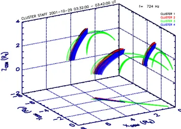
the equator (red), whereas they correspond to waves going to the equator for SC3 (blue). It is also observed that the frequency bandwidth of these waves going to the equator for SC3 does not cover exactly the corresponding frequency bandwidth of the peaks observed in Fig. 8, as it did in the first case. The results of the multiple ray tracing for each polar and azimuthal determinations between 03:32 and 03:42 UT are given in Fig. 9 for a frequency equal to 724 Hz. Fig-ure 9 represents the 3-D plots of the rays in GSM coordinates and their corresponding projections on the three planes. The number of SC3 rays is not so important but, as in the first time interval, it is observed that all SC record waves span-ning the same equatorial region. SC3 observes these waves after a LHR reflection.

5 Discussions and conclusion

The ray tracing shows that, at the same time, direct waves are emitted from the equator (the chorus source region) and re-flected waves come through the same equatorial region. The origin of these reflected waves must be the same as the main chorus emission (a hiss emission going through the equator would not have enough intensity to be observed after a

re-Fig. 9. Plots of the ray traces in 3-D and their corresponding projec-tions on the three planes for the time interval 03:32–03:42 UT and for a frequency equal to 724 Hz.

flection). Then, for the first time it was possible to simultane-ously observe waves directly emitted from the source region and the same waves returning to the equator after a LHR re-flection. At least two satellites are necessary to find (using the ray tracing) that, for example, in case 1 of Fig. 2, the two emissions seen at the same time, at the same frequency, but not at the same location on SC1 (SC2, or SC4) and SC3 (one being directed toward the equator and the other away from the equator), have the same origin, and then to demonstrate that we have observed a reflected wave. This opportunity is due to the simultaneous data recording on the four CLUS-TER SC and also to the particular configuration of their or-bits during this day. SC3 was nearly on the same orbit as the others but with a delay of 30 min. Correspondences between the meridian lines of, on the one hand, SC3 and, on the other, hand SC1, SC2, and SC4, can also be seen on the XY GSE planes of Figs. 5b (first time interval) and 9 (fourth time in-terval) where their traces point in the same direction. It is not the case in Figs. 7a (second time interval) and 7b (third time interval) where SC3 and the other three SCs observe waves coming from different source regions.

The discrepancy that is observed in the first interval be-tween the peak in Fig. 4 located around 456 Hz and the fre-quency bandwidth of waves returning to the equator (red area in Fig. 2) can be explained by the experimental configuration of the STAFF-SA experiment (the situation is similar for the fourth interval). This frequency bandwidth in Fig. 2 is com-prised between 600 and 1000 Hz, which corresponds to the frequency sub-band of analysis C (see Sect. 2). It means that analysis in this frequency sub-band gives a better spectral matrix estimation due to a larger number of averaged spec-tra relative to the frequency sub-bands B and A. Due to this fact, the estimation of the wave propagation parameters that are derived from the spectral matrix is also much better in the sub-band C. In this event where the wave maximum oc-curs in the sub-band B, the reliability of the analysis result

(10)

M. Parrot et al.: Magnetospherically reflected chorus waves 1119 for the sign of the z-component of the Poynting vector is not

excellent (mixture of red and yellow values below 512 Hz in Fig. 2). This difference between the sub-bands B and C is clearly seen in the last four panels of Fig. 2.

The fact that in Fig. 6a, SC4 does not map correctly the source at a frequency equal to 456 Hz can be due to its loca-tion relative to SC1 and SC2. It is seen in Fig. 3b that, at the beginning and especially during the first time interval, SC4 is not exactly on the same meridian line. It could explain that SC4 receives waves coming from a different region.

Cornilleau-Wehrlin et al. (1985) have studied the in-teraction between energetic electrons and whistler mode ELF/VLF magnetic waves measured by GEOS. They deter-mined the spatial growth rate of these waves and, therefore, they deduced that the corresponding reflection coefficient at the ionosphere for the wave power intensity must be of the order of 0.05. In the present study, it is possible to experi-mentally measure this coefficient which is directly given by plots in Figs. 4 and 8. In the first case (Fig. 4), the ratio for the magnetic and electric power spectral densities at 400 Hz between SC3 and the three others is 0.005 and 0.001, respec-tively. The ratio for the fourth case (Fig. 8) is 0.01 and 0.003, respectively. This of course depends on the plasma parame-ters along the reflected wave path during this particular day, but it is observed that the experimental magnetic ratio ob-tained in the two cases fits the theoretical one obob-tained by Cornilleau-Wehrlin et al. (1985).

Goldstein and Tsurutani (1984) and Hayakawa et al. (1984) have shown that the wave normal of chorus el-ements at frequencies lower than one-half the electron gy-rofrequency is close to the Earth’s magnetic field at the equa-tor, which seems to indicate that the generation mechanism could be due to electron cyclotron instability. It is interesting to check the values of the polar angle θ of waves returning to the equator during this event. Looking at the four bot-tom panels of Fig. 2, these waves approach the equator in three cases (around 1 kHz, blue colour): on SC1 and SC2 at

∼02:48 UT, and on SC3 at ∼03:28 UT. All cases indicate a

similar feature, as it can be seen on the top panels of Fig. 2. When the satellites get closer to the equator the polar

an-gle θ moves to values less than 20◦. Goldstein and

Tsuru-tani (1984) concluded that the wave growth is maximum for waves propagating parallel to the Earth’s magnetic field at the magnetic equator where this magnetic field is minimum. Therefore, it can be expected that the waves returning to the equator will endure a further amplification. A more detailed study of the wave normal angle of chorus emissions recorded by CLUSTER will be published elsewhere.

With this ray tracing study it is also possible to evaluate the minimum size of the chorus source. In this event which is at around 08:40 MLT (Magnetic Local Time), the X-extension

of the source is between 3.5 and 4.5 RE, and the Y -extension

is between 4.5 and 6.5 REat a frequency equal to 724 Hz. In

a further work, dimensions of the chorus sources at the equa-tor will be extensively studied for different magnetic local times and different magnetic activities.

Acknowledgements. Thanks are due to the Pis of the FGM (A. Balogh), WHISPER (P. D´ecreau) and EFW (M. Andr´e) experiments for the use of their data, and to the Hungarian Cluster Data Center, which provides auxiliary data. ESA and CNES are thanked for their support for the STAFF experiment.

Topical Editor T. Pulkkinen thanks J. Pickett and another referee for their help in evaluating this paper.

References

Balogh, A., Dunlop, M. W., Cowley, S. W. H., Southwood, D. J., Thomlinson, J. G., Glassmeier, K. H., Musmann, G., L¨uhr, H., Buchert, S., Acu˜na, M. H., Fairfield, D. H., Slavin, J. A., Riedler, W., Schwingenschuh, K., Kivelson, M. G., and the Cluster mag-netometer team: The Cluster magnetic field investigation, Space Science Rev., 79, 65–91, 1997.

Burtis, W. J. and Helliwell, R. A.: Banded chorus: A new type of VLF radiation observed in the magnetosphere by OGO-1 and OGO-3, J. Geophys. Res., 74, 3002–3010, 1969.

Burton, R. K. and Holzer, R. E.: The origin and propagation of chorus in the outer magnetosphere, J. Geophys. Res., 79, 1014– 1023, 1974.

Cairo, L. and Lefeuvre, F.: Localization of sources of ELF/VLF hiss observed in the magnetosphere: Three-dimensional ray tracing, J. Geophys. Res., 91, 4352–4364, 1986.

Cerisier, J. C.: Propagation perpendiculaire au voisinage de la fr´equence de la r´esonance hybride basse, in Plasma Waves in Space and in the Laboratory, 2, pp. 487–521, Edinburgh Uni-versity Press, Edinburgh, 1970.

Cornilleau-Wehrlin, N., Solomon, J., Korth, A., and Kremser, G.: Experimental study of the relationship between energetic elec-trons and ELF waves observed on GEOS: A support to quasi-linear theory, J. Geophys. Res., 90 (A5), 4141–4154, 1985. Cornilleau-Wehrlin, N., Chauveau, P., Louis, S., Meyer, A., Nappa,

J. M., Perraut, S., Rezeau, L., Robert, P., Roux, A., de Villedary, C., de Conchy, Y., Friel, L., Harvey, C. C., Hubert, D., Lacombe, C., Manning, R., Wouters, F., Lefeuvre, F., Parrot, M., Pinc¸on, J. L., Poirier, B., Kofman, W., Louarn, P., and the STAFF investiga-tor team: The CLUSTER STAFF experiment (Spatio Temporal Analysis of Field Fluctuations Experiment), Space Science Rev., 79, 107–136, 1997.

Cornilleau-Wehrlin, N., Chanteur, G., Rezeau, L., Parrot, M., Pinc¸on, J. L., and STAFF team: The CLUSTER STAFF exper-iment specific multi-point analysis, Proc. CLUSTER-II Work-shop on Multiscale / Multipoint Plasma Measurements, London, 22–24 September 1999, ESA SP-449, February 2000.

Cornilleau-Wehrlin, N., Chanteur, G., Perraut, S., Rezeau, L., Robert, P., Roux, A., de Villedary, C., Canu, P., Maksimovic, M., de Conchy, Y., Hubert, D., Lacombe, C., Lefeuvre, F., Par-rot, M., Pinçon, J. L., Décréau, P. M. E., Harvey, C. C., Louarn, Ph., Kofman, W., Santol´ık, O., Alleyne, H. St. C., Roth, M., and STAFF team: First results obtained by the Cluster STAFF exper-iment, Ann. Geophysicae, 21, 437–456, 2003.

Daly, P. W.: Users guide to the CLUSTER Science Data Sys-tem, DS-MPA-TN-0015, 19 April 2002, ftp://ftp.estec.esa.nl/ pub/csds/task for/users guide/csds guide.html, 2002.

Décréau, P. M. E., Fergeau, P., Krasnosels’kikh, V., Lévêque, M., Martin, Ph., Randriamboarison, O., Sené, F. X., Trotignon, J. G., Canu, P., Mögensen, P. B., and the Whisper experimenters: Whisper, a resonance sounder and wave analyser: performances

(11)

and perspectives for the Cluster mission, Space Sci. Rev., 79, 157–193, 1997.

Décreau, P. M. E., Fergeau, P., Krasnoselskikh, V., Le Guirriec, E., Lévêque, M., Martin, Ph., Randriamboarison, O., Rauch, J. L., Sené, F. X., Séran, H. C., Trotignon, J. G., Canu, P., Cornil-leau, N., de Féraudy, H., Alleyne, H., Yearby, K., Mögensen, P. B., Gustafsson, G., André, M., Gurnett, D. C., Darrouzet, F., Lemaire, J., Harvey, C. C., Travnicek, P., and Whisper experi-menters: Early results from the Whisper instrument on Cluster: an overview, Ann. Geophysicae, 19, 1241–1258, 2001.

Dunkel, N. and Helliwell, R.: Whistler mode emissions in the OGO 1 satellite, J. Geophys. Res., 74, 6371–6385, 1969.

Goldstein, B. E. and Tsurutani, B. T.: Wave normal directions of chorus near the equatorial source region, J. Geophys. Res., 89, 2789–2810, 1984.

Gustafsson, G., Andr´e, M., Carozzi, T., Eriksson, A. I., F¨althammar, C.-G., Grard, R., Holmgren, G., Holtet, J. A., Ivchenko, N., Karlsson, T., Khotyaintsev, Y., Klimov, S., Laakso, H., Lindqvist, P.-A., Lybekk, B., Marklund, G., Mozer, F., Mur-sula, K., Pedersen, A., Popielawska, B., Savin, S., Stasiewicz, K., Tanskanen, P., Vaivads, A., and Wahlund, J.-E.: First results of electric field and density observations by Cluster EFW based on initial months of operation, Ann. Geophysicae, 19, 1219–1240, 2001.

Hayakawa, M., Yamanaka, Y., Parrot, M., and Lefeuvre, F.: The wave normals of magnetospheric chorus emissions observed on board GEOS 2, J. Geophys. Res., 89, 2811–2821, 1984. Kennel, C. F. and Petscheck, H. E.: Limit on stably trapped particle

fluxes, J. Geophys. Res., 71, 1–28, 1966.

Kimura, I.: Effects of ions on whistler-mode ray tracing, Radio Sci-ence, 1(3), 269–283, 1966.

LeDocq, M. J., Gurnett, D. A., and Hospodarsky, G. B.: Chorus source locations from VLF Poynting flux measurements with the Polar spacecraft, Geophys. Res. Lett., 25 (21), 4063–4066, 1998. Lefeuvre F. and Parrot, M.: The use of the coherence function for the automatic recognition of chorus and hiss observed by GEOS-1, J. Atmos. Terr. Phys., 4GEOS-1, 143–152, 1979.

Means, J. D.: Use of the three-dimensional covariance matrix in analyzing the polarisation properties of plane waves, J. Geophys. Res., 77, 5551–5559, 1972.

Meredith, N. P., Horne, R. B., and Anderson, R. R.: Substorm de-pendence of chorus amplitudes: Implications for the accelera-tion of electrons to relativistic energies, J. Geophys. Res., 106,

13 165–13 178, 2001.

Muto, H. and Hayakawa, M.: Ray-tracing study of the propagation in the magnetosphere of whistler-mode VLF emissions with fre-quency above one half the gyrofrefre-quency, Planet. Space Sci., 35, 1397–1404, 1987.

Nagano, I., Yagitani, S., Kojima, H., and Matsumoto, H.: Analysis of wave normal and Poynting vectors of the chorus emissions observed by Geotail, J. Geomagn. Geoelectr., 48, 299–307, 1996. Parrot, M., Santol´ık, O., Cornilleau-Wehrlin, N., Maksimovic, M., and Harvey, C. C.: Source location of chorus emissions observed by CLUSTER, Ann. Geophysicae, 21, 473–480, 2003.

Pedersen, A., Cornilleau-Wehrlin, N., de la Porte, B., Roux, A., Bouabdellah, A., Décréau, P. M. E., Lefeuvre, F., Sené, F. X., Gurnett, D., Huff, R., Gustafsson, G., Holmgren, G., Woollis-croft, L. J. C., Thompson, J. A., and Davies, P. H. N.: The Wave Experiment Consortium (WEC), Space Sci. Rev., 79, 93–106, 1997.

Santol´ık, O.: Propagation Analysis of Staff-SA Data with Co-herency Tests, LPCE/NTS/073.C, Lab. Phys. Chimie Envi-ron./CNRS, Orl´eans, France, 2001.

Santol´ık, O. and Parrot, M.: Propagation analysis of electromag-netic waves between the helium and proton gyro-frequencies in the low-altitude auroral zone, J. Geophys. Res., 103, 20 469– 20 480, 1998.

Santol´ık, O. and Parrot, M.: Case studies on wave propagation and polarisation of ELF emissions observed by Freja around the local proton gyro-frequency, J. Geophys. Res., 104, 2459–2476, 1999. Santol´ık, O., Lefeuvre, F., Parrot, M., and Rauch, J. L.: Complete wave-vector directions of electromagnetic emissions: Applica-tions to INTERBALL-2 measurements in the night-side auroral zone, J. Geophys. Res., 106, 13 191–13 201, 2001.

Sazhin, S. S. and Hayakawa, M.: Magnetospheric chorus emissions: A review, Planet. Space Sci., 40, 681–697, 1992.

Tsurutani, B. T. and Smith, E. J.: Postmidnight chorus: a substorm phenomenon, J. Geophys. Res., 79, 118–127, 1974.

Tsurutani, B. T. and Smith, E. J.: Two types of magnetospheric ELF chorus and their substorm dependences, J. Geophys. Res., 82, 5112–5128, 1977.

Tsurutani, B. T., Smith, E. J., West, Jr., H. I., and Buck, R. M.: Chorus, Energetic electrons and magnetospheric substorms, in: Wave Instabilities in Space Plasmas, (Eds) Palmadesso, P. J. and Papadopoulos, K., D. Reidel Publishing Company, 55–62, 1979.