HAL Id: hal-01712164
https://hal.archives-ouvertes.fr/hal-01712164
Submitted on 22 Mar 2018
HAL is a multi-disciplinary open access archive for the deposit and dissemination of sci-entific research documents, whether they are pub-lished or not. The documents may come from teaching and research institutions in France or abroad, or from public or private research centers.
L’archive ouverte pluridisciplinaire HAL, est destinée au dépôt et à la diffusion de documents scientifiques de niveau recherche, publiés ou non, émanant des établissements d’enseignement et de recherche français ou étrangers, des laboratoires publics ou privés.
A net-exchange Monte Carlo approach to radiation in
optically thick systems
A de Lataillade, J. L. Dufresne, Mouna El-Hafi, Vincent Eymet, R Fournier
To cite this version:
A de Lataillade, J. L. Dufresne, Mouna El-Hafi, Vincent Eymet, R Fournier. A net-exchange Monte Carlo approach to radiation in optically thick systems. Journal of Quantitative Spectroscopy and Ra-diative Transfer, Elsevier, 2002, 74 (5), pp.563-584. �10.1016/S0022-4073(01)00272-2�. �hal-01712164�
A net-exchange Monte Carlo approach to radiation in
optically thick systems
A. de Lataillade
a; ∗, J.L. Dufresne
b, M. El Ha!
a, V. Eymet
c, R. Fournier
caCentre Energ!etique-Environnement, UMR CNRS 2392 Ecole des Mines d’Albi-Carmaux,
31 all!ees des Sciences, 81000 Albi CT, Cedex 09, France
bLMD=CNRS, Universit!e de Paris VI, 75252 Paris, France cLESETH, Universit!e Paul Sabatier, 31077 Toulouse, France
Abstract
A Monte Carlo approach to radiative transfer in participating media is described and tested. It solves to a large extent the well known problem of Monte Carlo simulation of optically thick absorption con!gurations. The approach which is based on a net-exchange formulation and on adapted optical path sampling procedures is carefully designed to insure satisfactory convergence for all types of optical thicknesses. The need for such adapted algorithms is mainly related to the problem of gaseous line spectra representation in which extremely large ranges of optical thicknesses may be simultaneously encountered. The algorithm is tested against various band average computations for simple geometries using the Malkmus statistical narrow band model. ? 2002 Elsevier Science Ltd. All rights reserved.
Keywords: Monte Carlo; Sampling optimization; Line spectra; Net-exchange formulations
1. Introduction
Since the emergence of computational physics, Monte Carlo methods have been extensively used for numerical simulation of radiative heat transfer in participating media. They !rst appeared as strict numerical implementations of photon transport stochastical models [1,2]. As such, they were commonly quali!ed by “exactness” and were mainly used for production of reference solutions in the process of validating other numerically more e"cient simulation techniques.
∗Corresponding author. Present address: CERFACS, 42 avenue Gaspard Coriolis, 31057 Toulouse Cedex 01, France.
Recent research e#orts depart from this original position in three ways [3,5]:
(1) underlying physical formulations are intensively rediscussed (reverse formulations, net-exchange formulations), sometimes preserving very little similitude with photon transport models;
(2) intensive use is made of all available convergence enhancement techniques;
(3) the emergence of massively parallel hardware allows one to seriously consider statistical methods for operational use (and not only for reference solution production), in particular when thinking of the di"culties encountered with deterministic techniques in front of detailed three-dimensional geometries and complex spectral properties.
Among the strongest handicaps of today’s Monte Carlo algorithms, are the di"culties related to numerical behavior in the optically thick limit [4,5]. In case of very short photon mean free paths, most bundles are absorbed in the vicinity of their emission positions which means that only very few bundles e#ectively participate to distant radiative transfers. The consequence is that Monte Carlo algorithms based on bundle transport formulations require very large numbers of statistical realizations for su"ciently accurate radiative exchange estimations. For less intuitive reasons, as we will illustrate hereafter, path integrated Monte Carlo algorithms encounter similar di"culties.1
The other numerical di"culty encountered with optically thick media is related to spatial dis-cretization. Computational costs impose constraints to geometrical grid sizes that cannot be reduced su"ciently for the optically thin assumption to be valid. It therefore becomes essential to account for sub-grid scale temperature pro!les. In the optically thick limit indeed, the radiative net-exchange between adjacent volumes is proportional to temperature gradients at the interface (di#usion assump-tion) and the assumption of isothermal meshes would lead to strong energy net-exchange overestima-tions. This constraint requires that Monte Carlo algorithms do not consider global mesh emissions, starting from mesh boundaries, but instead reduce the physical description to local sub-grid emissions, as a function of sub-grid temperature pro!les, through random generations of emission positions [6]. These questions are particularly sensitive in gaseous media as line spectra induce wide ranges of optical thicknesses; the optically thick limit being rapidly encountered in the spectral vicinity of absorption line centers. Solutions were proposed in [4,7,8] to overcome this speci!c di"culty on the basis of hybrid algorithms, combining Monte Carlo with di#usion algorithms. However, such hybrid algorithms face two new di"culties: that related to the criteria used when switching from one model to the other, and that related to the behavior of di#usion models in the vicinity of surface boundaries. Among recent attempts, Cherkaoui et al. [6,9] showed, for quasi-isothermal H2O–CO2–
air mixtures, using a narrow band statistical model [10], that thanks to intrinsic reciprocity principle satisfaction, net exchange Monte Carlo algorithms were much less sensitive to optical thickness than standard or reverse Monte Carlo algorithms. However, the spatial integration procedure could not be simply optimized on the basis of average transmission functions. The required computational e#ort, although much smaller than for standard algorithms, still increased signi!cantly as a function of optical thickness.
1In the present text, the terminology “bundle transport algorithm” will be used for algorithms in which energy is
distributed via emission of energy bundles, each of which is entirely absorbed at a single stochastically determined location. The alternative terminology “path integrated algorithm” will denote algorithms in which bundle energy is exponentially distributed along stochastically determined semi-in!nite optical paths.
We now present such a net exchange Monte Carlo approach devoted to gaseous radiation simu-lation. Di#erences with [6] are essentially that:
• spectral integrations are performed with a k-distribution model, randomly generating monochro-matic absorption coe"cients [11,12] instead of using narrow-band average transmission functions; • a path integrated algorithm is used instead of a bundle transport algorithm;
• sub-grid temperature integrations are signi!cantly optimized by physical and mathematical simpli!-cations associated with the k-distribution spectral formulation (exponential extinction and bypassing of spectral correlation di"culties [13–18]).
Section 2 begins on a monochromatic basis with simple one-dimensional geometries, discussing spatial integration procedures. Generalization is then made to any geometries. At this stage a net-exchange re-formulation is further introduced and convergence illustrations are made on the basis of simple one-dimensional slab con!gurations.
Section 3 introduces the k-distributions Monte Carlo spectral integration approach, discussing sampling probability choices. The same test case is used for convergence illustrations considering narrow-band integrated radiative powers, on the basis of Malkmus model [10], for a wide range of line overlap parameters and average optical thicknesses.
2. Optics and geometries
Using k-distribution approaches for spectral integration allows one to consider all optic and ge-ometric integrations on a pseudo-monochromatic basis (see Section 3). Transmission functions are therefore exponential functions, which in the frame of MC integration allows simple variance reduc-tion techniques to be implemented, in particular as far as sub-grid integrareduc-tion is concerned. For the sake of clarity, in the present section, optic and geometry are discussed assuming a non-scattering, uniformly absorbing medium. Both assumptions may be easily relaxed as in any standard Monte Carlo algorithm.2
2.1. Sub-grid integration
In order to illustrate the behavior of standard MC algorithms as function of optical thickness and to introduce the principle of the proposed algorithm, the simple problem of monochromatic slab emission is !rst analysed. This permits the derivation of analytical solutions and associated variances from which our choices of optimized probability density functions may be physically discussed and tested.
Consider a horizontal slab of semi-transparent medium between black boundaries. The slab thick-ness is L and the downward unit vector normal to the slab is written ˜n (see Fig. 1). The temperature
2Scattering is usually represented via random generation of scattering positions and angles, the MC algorithm being
kept unchanged on the basis of broken lines optical paths instead of straight lines [2]. Non-homogeneous absorption creates no source of di"culty provided that the variations of absorption coe"cient are known along each optical path, which in the frame of the k-distribution approach may be achieved using the correlated-k assumption [13,17].
Fig. 1. Non isothermal 1D slab con!guration —–: linear blackbody intensity pro!le; - - - parabolic blackbody in-tensity pro!le.
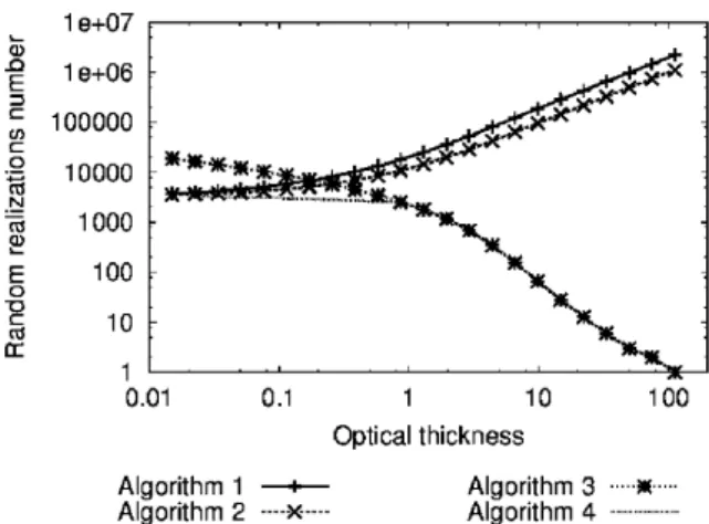
Fig. 2. Number of required bundle realizations for MC es-timation of inhomogeneous slab emission with a 1% rel-ative error, as function of slab optical thickness. Results corresponding to Algorithms 1, 2 and 3 are analytical, whereas the results of Algorithm 4 were obtained with e#ective MC simulations.
pro!le is such that the monochromatic blackbody intensity at the considered frequency follows a linear pro!le from B0 at the bottom to 0 at the top.
Downward radiative $ux at the bottom can be expressed as F =! 2! d!(˜u)! L 0 dz k exp " − kz ˜u · ˜n # B0(1 − z=L) = 2!B0 " 1=2 − 3kL1 + E4(kL) kL # ; (1)
where En is the nth exponential integral.
Algorithm 1. In the most straightforward MC algorithm; sampling events are randomly generated in a way that preserves a close analogy with photon transport statistics. As far as the present test case is concerned; z and ˜u are sampled according to respectively uniform and isotropic probability density functions. F is then estimated counting bundles reaching the bottom boundary before absorption; which may be formally represented via the following expression:
F =! L 0 dz pZ(z) ! 2! d!(˜u)p"(˜u) ! +∞ 0 d# p$(#) w1(z;˜u; #) (2) with w1(z;˜u; #) = 2kL!B0(1 − z=L)S$# − z ˜u · ˜n% ;
where S is a step function: S(a) = 0 if a ¡ 0 and S(a) = 1 otherwise. The position of emission in the one-dimensional slab is produced by generating randomly the abscissa z according to pZ(z)=1=L.
The direction of emission is generated according to p"(˜u)=1=2!. Then z and ˜u de!ne a line of sight
and +∞: p$(#)=k exp(−k#). This leads to a bundle weight w1=w∗1(z)=2kL!B0(1−z=L) when the
bundle reaches the bottom boundary; w1= 0 otherwise. The radiative $ux addressed corresponds to
the average weight: F = ⟨w1⟩. The practical algorithm uses a !nite number N of emission-absorption
events to estimate F as the average of corresponding weights and such an estimate is associated with a statistical error
E%; 1=
& 1
N(⟨w21⟩ − ⟨w1⟩2): (3)
In the present simple case; this error can be obtained analytically as E%; 1= 2!B√ 0 N ' kL 2 − 2 kLE5(kL) − 2 3+ 1 4kL − " F 2!B0 #2 :
The “pathological” behavior of such MC algorithms for strong optical thicknesses can be seen noticing that E%; 1=F ≃ (2kL=N when kL!1 and therefore that the relative error tends to in!nity
when optical thickness tends to in!nity. Fig. 2 displays the number of random generations required for a 1% relative error as a function of optical thickness. In terms of physical images, this behavior can be explained by the fact that for strong optical thicknesses, most bundles are absorbed within the slab; therefore only a few bundles contribute to the radiative $ux at the boundary and the statistics require large numbers of emitted bundles for satisfactory accuracies.
Algorithm 2. This interpretation could lead one to believe that path integrated MC algorithms; in which all bundles leave the emitting volume element (no complete self absorption); would have better statistical behaviors. In these algorithms; bundles are emitted as described above with the same initial weight w∗
2(z) = w∗1(z); but instead of being absorbed at one single absorption position;
each bundle undergoes an exponential attenuation along the de!ned ray until the bottom boundary is encountered. In our case; such an algorithm corresponds to the following formulation:
F =! L
0
dz pZ(z)
!
2!
d!(˜u)p"(˜u)w2(z;˜u) (4)
with w2(z;˜u) = 2kL!B0(1 − z=L) exp " −˜u · ˜nkz # :
Events are de!ned with only two random generations (emission position and direction; no absorption position). As before; F = ⟨w2⟩ and for a practical MC calculation with N events; the statistical error
is E%; 2= 2!B√ 0 N ' kL 4 − 1 4kLE5(2kL) − 1 6 + 1 16kL − " F 2!B0 #2 :
For strong optical thicknesses; this relative error simpli!es to E%; 2=F ≃ (kL=N; which is better than
that of a straightforward bundle transport algorithm but still tends to in!nity with increasing optical thicknesses. Path integrated algorithms therefore encounter equivalent bad behaviors. The reason is
that; although complete auto-absorptions have been suppressed; only bundles emitted in the immediate vicinity of the boundary leave the volume with a signi!cant weight; all other bundles are strongly attenuated and reach the boundary with a quasi-zero weight. The statistical di"culties are therefore very similar. The number of bundles required for a one percent relative error with Algorithm 2 are displayed in Fig. 2 and can be compared with that of Algorithm 1.
Algorithm 3. In both the above cases; the di"culties are obviously associated with emission position random generations. These di"culties can be relieved by modi!cation of pZ(z) to choose emission
positions close to the boundaries. However; exponential extinction depends on emission angles and radiation may come from further inside the slab for quasi-normal directions whereas only the very bottom of the slab contributes to quasi-tangential $uxes. It appears therefore that angular and spatial integrals ought to be inverted and emission directions generated before emission positions. If the direction ˜u is generated !rst; an adapted pdf of z knowing ˜u can be chosen to match exactly the exponential attenuation from z to the boundary. This adapted pdf is:
pZ; a(z;˜u) = k ˜u · ˜nexp " −˜u · ˜nkz # 1 − exp " −˜u · ˜nkL # : (5)
As for all biased MC algorithms; the bundle weight must be adjusted in accordance with the new pdf choice; which implies here that the previous bundle weight w∗
2(z) should be replaced by 1 − exp " −˜u · ˜nkL # exp " − kz ˜u · ˜n # 2!(˜u · ˜n)B0(1 − z=L):
The fact that ˜u ·˜n appears as product in this bundle weight expression would introduce an undesired distribution width in the optically thick limit. As a !rst step; to illustrate that MC algorithms may be simply adapted to deal with optically thick con!gurations; this di"culty can be bypassed via a modi!cation of the angular distribution using p"; l(˜u;˜n) = ˜u · ˜n=!. The initial bundle weight then
becomes w∗ 3(z) = 1 − exp " − kL ˜u · ˜n # exp " −˜u · ˜nkz # !B0(1 − z=L):
Altogether; the corresponding optimized algorithm consists of the following: (i) directions are gener-ated randomly according to p"; l(˜u;˜n) which corresponds to a Lambert angular distribution;
(ii) positions are alloted randomly according to the exponential distribution pZ; a(z;˜u); (iii)
bun-dles are alloted the initial weight w∗
3(z); (iv) the rest of the algorithm is kept unchanged; either a
bundle transport or a path integrated algorithm. Applying this algorithm in its ray-tracing form to the same test case as above corresponds formally to the following expression:
F =! 2! d!(˜u) p"; l(˜u;˜n) ! L 0 dz pZ; a(z;˜u)w3(z;˜u) (6)
with w3(z;˜u) = ) 1 − exp " − kL ˜u · ˜n #* !B0(1 − z=L)
and the corresponding statistical error is E3= 2!B√ 0 N ' 1 4 − 1 3kL + 1 4(kL)2 − 2E5(kL) k2L2 − E3(kL) 2 − 1 kLE4(kL) + E5(2kL) k2L2 − " F 2!B0 #2 :
Unlike the other two algorithms; the relative error does not tend to in!nity with increasing optical thickness; but instead decreases to zero as E3=F ≃ (1=3kL)(5=N. Fig. 2 displays the numbers of
bundles required to reach a 1% relative error and illustrates that the adapted algorithm encounters no speci!c di"culty for strong optical thicknesses.
Algorithm 4. This last Algorithm 3 shows however worse behavior than the two preceding in the optically thin limit. Such behavior is due to angular integration: the Lambert distribution (p"; l(˜u;˜n) = ˜u ·˜n=!) is indeed adapted to optically thick system emissions but not to thin ones that
tend to isotropy (p"(˜u) = 1=2!). This dependence on optical thickness may for instance be
ap-proached using an angular pdf that combines both limit cases:
• The Lambert law is kept for systems with optical thickness greater than unity: p"; a(˜u;˜n; kL) = p"; l(˜u) if kL ¿ 1
• For systems with optical thickness lower than unity; a Lambert like distribution is used for slab tangential directions and a uniform distribution for close to normal directions:
p"; a(˜u;˜n; kL) = 1 1 − kL=2 " S(kL− ˜u · ˜n) 1 2kL˜u · ˜n! + S(˜u · ˜n − kL) 1 2! # : (7)
The algorithm then formally corresponds to F = ! 2! d!(˜u)p"; a(˜u;˜n; kL) ! L 0 dz pZ; a(z;˜u)w4(z;˜u) (8) with
w4(z;˜u) = w3(z;˜u) p"; l(˜u;˜n)
p"; a(˜u;˜n; kL):
Numerical results obtained with Algorithm 4 are reported in Fig. 2 showing good behavior in both optically thin and optically thick limits.
2.2. Generalized algorithmic procedure
The preceding simple example (Monte Carlo estimation of the power emitted from a non-isothermal slab to a surface) illustrated how important it is to work on both the formulation choice and the
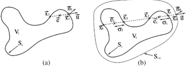
Fig. 3. Emission positions and emission directions. (a) In-tegration over the envelope. (b) InIn-tegration over a convex surrounding surface (see Appendix A).
Fig. 4. Absorption segments and exchange positions.
pdf adaptations to deal with optically thick conditions. A general three-dimensional Monte Carlo algorithm is presented hereafter that bene!ts from these observations concerning sub-grid integration optimization, generalizing the principle of Algorithm 4 to any geometry. For the sake of clarity, the algorithm is formally enunciated assuming black system boundaries, and the required extension associated with surface re$exions are rapidly treated via independent footnotes.
Let us consider a system divided into NV volume elements Vi of semi-transparent material and
NS opaque surface elements Si. Volume and surface elements are non-isothermal and the volume
elements cannot be assumed optically thin. The temperature !eld will be described as a continuous !eld and the corresponding blackbody intensity !eld at the considered frequency will be noted B(˜x) where ˜x is the coordinate vector.
When computing exchange rates from a volume to a surface, ’(Vi; Sj) (the radiative power emitted
by Vi that is absorbed by Sj), or between two volume elements, ’(Vi; Vj), with bundles starting from
Vi, the !rst step is the random generation of an emission position ˜e within Vi and of an emission
direction ˜u. The most direct extension of Algorithm 4 to three-dimensional geometries consists in the following procedure (see Appendix and Fig. 3a):
(1) A position ˜x1 is uniformly and randomly generated on Vi’s envelope, noted3 Si: pS(˜x1)=1=Si.
(2) The emission direction ˜u is randomly generated on the outward hemisphere at ˜x1 according to
the previously de!ned pdf adapted as function of Vi’s optical thickness: p"(˜u;˜n1; kL) (see Eq.
(7)) where ˜n1 is the outward oriented unit vector normal to Si at ˜x1. In the one dimensional
case the length L was chosen as the slab thickness, but in the general case L should be taken as a length scale characteristic of Vi’s thickness from ˜x1’s view point.
(3) ˜x1 and ˜u are used to de!ne a continuous segment within Vi from ˜x1 to ˜x2, where ˜x2 is the !rst
intersection with Si starting from ˜x1 in the direction −˜u.
(4) The emission position ˜e is randomly generated along the segment [˜x1;˜x2] according to an
expo-nential distribution:
˜e = ˜x1− #˜u with p$(#) = k exp(−k#)
1 − exp(−k∥˜x2− ˜x1∥):
3Depending on the geometries, generating ˜x
1on the envelope Si may be tedious, in which case the alternative procedure
At this stage, emission position and direction have been randomly generated to de!ne a line of sight leaving Vi at ˜x1. A bundle is then followed along this direction starting at ˜x1 with the following
initial bundle weight: w∗
0 = ! Si[1 − exp(−k∥˜x2− ˜x1∥)]pp"; l(˜u;˜n1)
"; a(˜u;˜n1; kL): (9)
As in any ray-tracing algorithm, the bundle weight is exponentially attenuated along its path as a function of the amount of encountered absorber. At any location ˜y, the remaining bundle weight is noted w∗(˜y) and satis!es w∗(˜y) ¡ w∗
0.
When computing ’(Vi; Sj) with N such emission events, each bundle is followed until Sj is
encountered at location ˜a. The Monte Carlo weight is then computed as
w(˜e;˜a) = w∗(˜a)B(˜e) (10)
and ’(Vi; Sj) is estimated as the average weight ⟨w⟩N. For optical paths where complete absorption
occurs before Sj is encountered, the event is attributed a weight4 w = 0.
Generally speaking, the line of sight intersects any volume element Vj in m segments [˜y2l−1; ˜y2l]
with l=1; : : : ; m (see Fig. 4). When computing ’(Vi; Vj), the ray is therefore followed until complete
absorption, de!ning these m segments and the Monte Carlo weight is computed as w(˜e; ˜y1; : : : ; ˜y2m) =
m
+
l=1
w∗(˜y2l
−1)[1 − exp(−k∥˜y2l− ˜y2l−1∥)]B(˜e): (11)
When computing ’(Si; Sj) and ’(Si; Vj) starting from Si, the algorithm is strictly similar in the limit
case of L = +∞: emission positions are generated uniformly on Si (# = 0); the angular
distribu-tion becomes Lambert distribudistribu-tion (p"; a(˜u;˜n1; +∞) = p"; l(˜u;˜n1)); and the initial weight becomes5
w∗
0 = !Si. The proposed algorithm allows therefore a continuous treatment of sub-system emissions,
from optically thin volumes to opaque surfaces, via optimized pdf choices for the total range of system optical thicknesses.
At this stage the algorithm is a forward algorithm in the sense that quantities addressed are exchange rates from one geometrical element to another. As discussed in the introduction section, net-exchange algorithms have been shown to ensure better convergence in numerous con!gurations.
4When simulating black boundary cavities, complete absorption occurs at the !rst boundary encounter and S j may
only be encountered once. In the case of re$ecting boundaries, the optical path is continued after each surface encounter generating randomly a re$exion direction according to the local directional–directional re$ectivity function. At each such re$exion, the weight is attenuated according to the directional absorptivity (w∗→ (1 − &)w∗) and the path is interrupted
when w∗¡ '=%Bmax is satis!ed, where ' is the required accuracy and %Bmax the maximum absolute blackbody intensity
di#erence between the emission point and any other location in the cavity. Such a multiple broken line optical path may encounter Sj at several locations ˜a1; : : : ;˜am under incident directions corresponding to directional absorptivities &1; : : : ; &m
and the MC weight is computed as
w(˜e;˜a1; : : : ;˜am) = m
+
l=1
&lw∗(˜al)B(˜e):
5In case of a non-black surface, w∗
For the sake of numerical quality, it is therefore preferable to further add this net-exchange reformu-lation step to the preceding algorithm which may be very simply performed thanks to the reciprocity principle. One may refer to [6,19] and [20] for details concerning net-exchange formulations, but the essential picture is that quantities addressed are net-exchange rates between geometrical elements. The net-exchange rate (Vi; Vj) between volumes Vi and Vj is the power emitted by Vi and absorbed
by Vj minus the power emitted by Vj and absorbed by Vi:
(Vi; Vj) = ’(Vi; Vj) − ’(Vj; Vi):
The radiative balance of any element is therefore the sum of all net-exchange rates with other discretization elements. Independently of the physical insight that net-exchange formulations may provide to radiative transfer problems, numerical bene!t associated with this formulation is that it intrinsically satis!es the reciprocity principle. Apart from con!gurations in which strongly irregular discretizations are required, one may think of con!gurations in which dominant radiative exchanges occur between elements at similar temperature levels. The reason why in such cases net-exchange formulations lead to better numerical behavior than standard forward formulations is simply that when two elements are at similar temperature levels the two reciprocal exchange rates are numerically close to each other. The di#erence between these two exchange rates, that is the contribution to the radiative balance, may therefore be very small compared to exchange rates themselves. A numerical estimation procedure based on independent exchange rates estimations may therefore lead to very high levels of uncertainties (di#erence of two approximate quantities of similar magnitudes). In numerical methods based on net-exchange formulations, the quantities addressed are directly the net-exchange rates between elements and this di#erence taking step is bypassed.
This is particularly relevant to optically thick con!gurations in which main radiative exchanges occur between adjacent elements and correspond to exchange locations that are very close to the interface. These locations are therefore likely to correspond to very similar temperature levels.
As shown in [19] our forward Monte Carlo algorithm may be turned into a net-exchange algorithm via an additional step of absorption location random generation within each absorption segment. In practice, this means that the algorithm is kept strictly identical to what was presented above except that each time an absorption segment [˜y2l−1; ˜y2l] is identi!ed. An absorption position ˜al is randomly
generated (as for emission) according to an exponential distribution: ˜al= ˜y2l−1+ #˜u with p$(#) = k exp(−k#)
1 − exp(−k∥˜y2l− ˜y2l−1∥):
Monte Carlo weights are then modi!ed by replacing blackbody intensities at the emission position B(˜e) by blackbody intensity di#erences between emission and absorption positions. Eqs. (10) and (11) therefore simply become
w(˜e;˜a) = w∗(˜a)[B(˜e) − B(˜a)] (12)
for interaction with a surface and w(˜e; ˜y1; : : : ; ˜y2m;˜a1; : : : ;˜am)
=
m
+
l=1
w∗(˜y2l
for interaction with a volume. The average values of these new Monte Carlo weights are now estimated from N realizations to approximate the net exchange rates (Vi; Sj) and (Vi; Vj) directly.
2.3. Convergence illustration (monochromatic)
Simple con!gurations (one dimension slab) are used for convergence quality illustration. Simula-tions are !rst performed on a monochromatic basis and similar examples are later reconsidered in Section 3 with an additional integration over gaseous line spectra.
The slab geometry is that of Fig. 1. The boundaries are black and absorption coe"cient is uniform. The !rst test case is that proposed in [5] for comparison of forward bundle transport algorithm, forward path integrated algorithm and reverse path integrated algorithm.6 The temperature pro!le is
such that the monochromatic blackbody intensity at the considered frequency is B0 at the boundaries
and uniform at B0+ %B across the slab. Estimated quantities are radiative $ux divergence averages
within each of the 10 regular layers used for slab discretization.
For slab optical thickness kL=10, Fig. 5 presents successively the exact and Monte Carlo solutions, the percent error presented in [5] for the three tested strategies (in the speci!c case of B0=0) and the
percent error reached with our proposed adapted net-exchange methodology (which is independent of B0 owing to the net-exchange formulation). All corresponding simulations are performed using
10,000 ray sampling per element. The conclusion of this !rst exercise is undoubtedly the same as that of Fig. 2: a simple reformulation of the emission position and emission angle integrals allows one to solve the well known problem of Monte Carlo convergence for optically thick con!gurations. To further illustrate this point, Fig. 6 displays the radiative $ux divergence averages (and statistical error) within layer 1 (against the boundary) and layer 5 (one of the two central layers) as a function of optical thickness widely above kL = 10. These simulations con!rm that in the proposed scheme statistical errors are insensitive to optical thickness in the optically thick limit.
However, this !rst test case is not very representative of practical optically thick con!gurations in which most of the physics lies in the energy redistribution process within the medium via short distance photon exchanges. Treatment of non-uniform temperature pro!les is essential keeping in mind the limiting case of the Rosseland approximation in which energy transfers are modeled on the basis of second order spatial derivatives (as for any di#usion process). In our second test case, the temperature pro!le is therefore chosen such that the monochromatic blackbody intensity at the considered frequency follows a parabolic pro!le across the slab, from B0 at the boundary to B0+%B
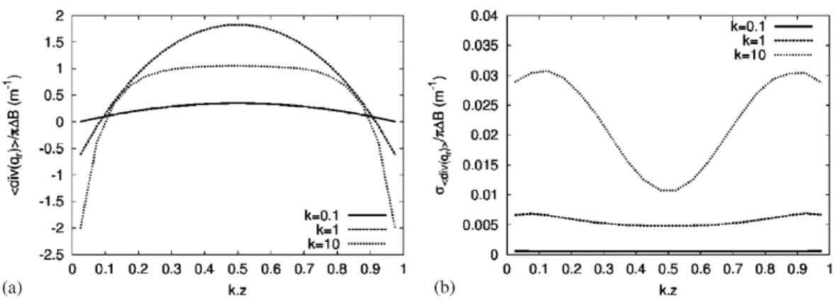
at the slab center. Slab discretization is now performed on the basis of 20 layers of equal width. Fig. 7 displays simulation results and statistical errors for three optical thicknesses (kL = 0:1, kL = 1 and kL = 10) for 10,000 ray samplings per element. Similarly, Fig. 8 displays the results obtained for layer 3 and layer 10 as a function of optical thickness.
Statistical errors are necessarily higher for this second test case than for the isothermal slab: sub-grid temperature pro!le integration is now essential whereas only the angular integration had to be statistically reconstructed in preceding test case. Worth some attention is the fact that errors are higher close to the boundaries than at the center of the slab. After a close look at this behavioral di#erence, it appears that this is not a boundary e#ect. It is related to the temperature pro!le only:
6The corresponding denominations used in [5] are the forward collision based algorithm, forward pathlength algorithm
Fig. 5. Comparison of the proposed net-exchange Monte-Carlo (NEMC) approach against “collision based”, “pathlength” and “reverse” algorithms as reported in [5]. The computations are on a monochromatic basis. The test case is a uniform one-dimensional slab at B0+ %B with black boundaries at B0 discretized in 10 regular layers. Presented quantities are
radiative $ux divergence averages for each layer normalized by !%B. 10,000 sampling events per discretization ele-ment are used for each algorithm. In [5] computations were performed with B0= 0 whereas NEMC behaviors are
in-sensitive to B0. (a) Analytical and NEMC solutions. (b) Percent errors as reported in [5]. (c) Percent errors as obtained
with NEMC.
Fig. 6. (a) Radiative $ux divergence averages for layer 1 (against the boundary) and layer 5 (at slab center) as functions of slab optical thickness for the same test case as in Fig. 5. (b) Corresponding MC standard deviation (statistical errors).
Fig. 7. (a) Estimated radiative $ux divergence averages, using the proposed net-exchange Monte-Carlo approach using 10,000 sampling events per discretization element. The test case is a 1D slab with black boundaries. Computations are held on a monochromatic basis. Absorption coe"cient is uniform. The blackbody intensity pro!le is parabolic from B0
at the boundaries to B0+ %B at the center. The slab is discretized in 20 regular layers. (b) Corresponding MC standard
deviation (statistical errors).
this pro!le is such that the second order spatial derivative of the monochromatic blackbody intensity is constant (which explains why the radiative $ux divergence tends to a $at pro!le when increasing optical thickness), but the net energy transfer rate of each layer is being computed essentially as the sum of two net-exchange rates with neighboring layers. Numerical conditions are very distinct for layer 3 and layer 10 for instance. For layer 3, blackbody intensity gradients are of similar mag-nitude at both interfaces and the net energy transfer rate is therefore computed as the di#erence of two uncertain net-exchange rates of similar magnitudes. Statistical errors on radiative net-exchanges are therefore ampli!ed by this di#erence taking step. This di"culty is not encountered with layer 10 because the parabolic pro!le is $at at the slab center which means that the net-exchange rate between layer 10 and layer 11 tends to zero with increasing absorption. Reducing this sensitivity of the algorithm to the sub-grid temperature pro!le could be partly achieved via an explicit representa-tion of this spatial dependence in the pdf choice for emission posirepresenta-tion sampling. But at the present stage, without a speci!c high accuracy requirement, the results seem quite acceptable (never more than a few percent error with 10,000 ray samplings), especially when thinking of complete diver-gences as are commonly encountered with standard Monte Carlo algorithms in the optically thick limit.
3. Spectral integration 3.1. Principles
In the preceding section, MC integrations were considered on a monochromatic basis, optimizing the algorithm in such a way that satisfactory convergence is ensured for all types of optical thick-nesses. The motivation for this optimization attempt was that when considering spectral integration over line spectra, a large range of optical thicknesses may be encountered from very high thicknesses at line centers to optically thin con!gurations between lines.
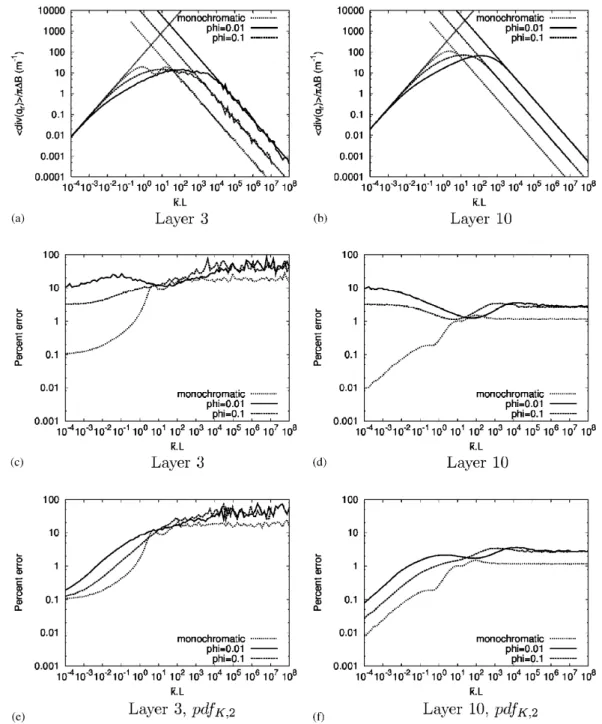
Fig. 8. Radiative $ux divergence averages (a and b) and standard deviations (statistical errors, c, d, e and f) for layer 3 and layer 10 as a function of slab optical thickness for the same test case as in Fig. 7. Also presented are computations performed on a narrow band interval using Malkmus model as a function of average optical thickness &kL for two values of the shape parameter (line overlap parameter): ( = 0:1 and ( = 0:01. Analytical solutions corresponding to the optically thin and optically thick models are presented as straight lines for comparison. Standard deviations in c and d correspond to the use of pdfK; 1(k) = f(k) for k-sampling, whereas e and f correspond to the use of pdfK; 2(k),
When computing integrated exchange (or net-exchange) rates over a spectral interval [%min; %max]
with a MC algorithm, the only step to be added to the preceding algorithms is the random generation of a frequency % within [%min; %max] according to an arbitrarily chosen pdf. As for optic and geometric
considerations, this pdf is essential in the sense that numerical convergence depends on its choice. In order to formalise this point, let us write the spectrally integrated net-exchange rate between volumes Vi and Vj using a synthetic path-integral formulation in which )%(Vi; Vj) is the space of
all possible optical paths *, at frequency %, and h (*; %) is the contribution of monochromatic net exchange along ): (Vi; Vj) = ! %max %min d% %(Vi; Vj) = ! %max %min d%! )%(Vi;Vj) d* h (*; %): (14) As before, pdf ’s are introduced for integration variables % and * and Monte Carlo estimates are obtained on the basis of corresponding sampling events:
(Vi; Vj) = ! %max %min d% pdfN(%)! )%(Vi;Vj) d* pdf)(*)w (*; %) ≈N1 N + n=1 w (*n; %n); (15)
where *n and %n are N random generations of optical path and frequency according to pdf) and
pdfN, and where the MC weight w is computed as w (*; %) = h (*; %)
pdfN(%)pdf)(*):
For a given frequency, optimizing optical path sampling was the object of Section 2: pdf)(*) is therefore nothing but a formal representation of spatial and angular sampling procedures that were carefully discussed above as a function of optical thickness. The remaining question is therefore that of optimizing the frequency pdf choice. In this optimization exercise, the variance of w (*n; %n) must
be as low as possible, keeping pdfN(%) simple enough to handle for practical random sampling. This compromise is extremely di"cult to reach when dealing with gaseous infrared spectra such as those of water vapor and carbon dioxide. The spectral variations of the radiative transfer functions to be integrated are so sharp and irregular that it seems not feasible to design su"ciently simple spectral pdf ’s that could compensate for h ’s variations.
Very strong simpli!cations may however be introduced when the spectral interval is narrow enough for blackbody intensities, surface re$exion properties and scattering properties to be assumed inde-pendent of frequency: this is the narrow band assumption that is a common basis for all so-called narrow band spectral integration models. Under this assumption, the function to be integrated de-pends only on frequency through the spectral dependence of absorption coe"cients, which o#ers the opportunity for narrow band k-distribution methodology to be applied:
• A new function ˜h is introduced that explicitly de!nes the absorption coe"cient dependence: h (*; %) = ˜h (*; k%).
• The distribution of absorption coe"cients within the interval [%min; %max] is noted f(k) (the inverse
transmission function [11]) and is modeled to the level of required accuracy.
• (Vi; Vj) may then be re-written in a way that justi!es a new MC algorithm in which random
absorption coe"cients are generated instead of random frequencies: (Vi; Vj) = [%max− %min] ! kmax kmin dk f(k)! )(Vi;Vj) d * ˜h (*; k) =! kmax kmin dk pdfK(k)! )(Vi;Vj) d* pdf)(*) ˜w (*; k) ≈N1 N + n=1 ˜ w (*n; kn) (16) with ˜ w (*; k) = [%max− %min]pdff(k) K(k) ˜h (*; k) pdf)(*):
Note that the frequency dependence of optical path domain )(Vi; Vj) vanishes owing to the narrow
band assumption.
The main advantage of such a formulation is that the variations of the product ˜h (*; k)f(k) with k are much less erratic than those of h (*; %) with frequency, so that optimizing the choice of pdfK becomes realistic.7 The task of adapting the k-sampling pdf choice to the considered con!guration
type was studied and illustrated in [12] and three limit cases were identi!ed: • For computation of net exchange rates between two black surfaces at distance l:
pdfK(k) = fss(k; l) = e−klf(k)= &+(l): (17)
• For computation of net exchange rates between an optically thin volume and a black surface at distance l:
pdfK(k) = fgs(k; l) = ke−klf(k)= &+′(l): (18)
• For computation of net exchange rates between two optically thin volumes at distance l:
pdfK(k) = fgg(k; l) = k2e−klf(k)= &+′′(l); (19)
where &+(l) is the average transmission function. Thanks to inverse Gaussian distribution properties, these pdf ’s are mathematically easy to handle, provided that the considered spectrum follows the Malkmus model [12]. In the general case, the best !tted Malkmus spectrum may be used, insuring
7In this presentation two distinct pdf ’s of k are introduced. The !rst one, f(k) is the physical distribution of k as it
appears in the considered spectrum. The second pdfK(k) is entirely arbitrary and serves only for the MC algorithm. It
is however mainly on the basis of physical considerations that pdfK may be adequately chosen, ensuring that statistical
!rst order representation of emission=absorption spectral correlations. As illustrated later, linear combinations of such limit case pdf ’s may be used for intermediate cases, but nevertheless the design of adapted k-sampling pdf ’s for each new con!guration family remains a key step of such MC simulation e#orts to insure fast numerical convergence.
When the spectral interval [%min; %max] is not narrow enough for the narrow band assumption to
be valid, the interval may be divided in Nb narrow bands of width %%j around %j. Di#erent inverse
transmission functions fj(k) are introduced for each narrow band and Eq. (14) is written:
(Vi; Vj) = Nb + b=1 %%b ! kmax;b kmin;b dk fb(k) ! )b(Vi;Vj) d* ˜h ; b(*; k) = Nb + b=1 Pb ! kmax;b kmin;b dk pdfK; b(k)! )b(Vi;Vj) d* pdf); b(*) ˜w (*; k; b) ≈N1 N + n=1 ˜ w (*n; kn; bn) (20) with ˜ w (*; k; b) = %%b Pb fb(k) pdfK; b(k) ˜h ; b(*; k) pdf); b(*):
As for continuous integrals, in the frame of MC methods, discrete sums may be handled via arbitrary choices of discrete probabilities. Here Nb probabilities P1; : : : ; PNb are introduced (,
Nb
b=1Pb= 1) and
narrow band index random generation are performed according to this weighting, which should be chosen to match as accurately as possible the relative contribution of each band to the !nal result. As discussed in [6] this unknown contribution may be estimated on the basis of simple physical reasoning, but here again the choice remains problem-dependant, and may require substantial e#ort for non-intuitive new con!gurations.
3.2. Convergence illustrations (narrow band)
This general methodology was implemented practically and tested in [21] for application to com-bustion con!gurations. We con!ne ourselves to academic test cases similar to those used in the preceding section in order to illustrate statistical convergence qualities as functions of average opti-cal thickness for di#erent types of gaseous spectra. Spectral integration is performed over a spectral band of width %% for which the narrow band assumption is valid. The Malkmus statistical narrow band model is used so that parametric analysis is performed by varying the band average absorption coe"cient &k and the shape parameter8 ,. This model is used here under its k-distribution form
[11,12].
With the same 20 layer discretization as for monochromatic simulations, Fig. 8 displays radia-tive $ux divergence averages and percent statistical errors for layer 3 and layer 10 as functions of
8The shape parameter also called the line overlap parameter: , = 2*=- where * is the half line width at half height and
average optical thickness &kL, for two values of the shape parameter that are typical of spectrally sep-arated gaseous spectra (, = 10−2 and , = 10−1). Convergence qualities associated with two distinct
k-sampling pdf ’s are compared in terms of statistical errors for a given number of sampling events. The !rst one corresponds to straightforward k-sampling according to the physical distribution of ab-sorption coe"cient within the considered spectral interval: pdfK; 1(k) = f(k) (Fig. 8c–d). The second was proposed in [21], for combustion applications, as an attempt to account for the dependence on k of pseudo-monochromatic radiative exchanges (Fig. 8e–f):
pdfK; 2(k) = &K(l)fgs(k; 0) + [1 − &K(l)]fss(k; 0) (21)
with
&K(l) =g
ss(1=l; 0) − &+(l)gss(1=l; l)
1 − &+(l) ;
where gss is the cumulative distribution of fss (see Eqs. (17) and (18)) and where the length l is
taken as l = L for surface emissions and l = L=20 for volume emission.
The physical reasoning leading to this adapted pdf choice is the following. In the present sys-tems the net radiative $ux at each boundary is the result of a net-exchange with a gas volume of characteristic length scale L. There is indeed no net-exchange with the opposite boundary surface because the surfaces are at the same temperature. In the case where the system may be considered optically thin, the net radiative $ux at each boundary may then be seen as a net-exchange between a black surface and an adjacent optically thin gas volume; consequently, not taking into account volume temperature inhomogeneities, the best adapted k-sampling pdf is pdfK(k) = fgs(k; 0). At the
other extreme, where the system may be considered optically thick, always putting aside volume temperature inhomogeneities, the net radiative $ux may be seen as the result of a net-exchange between two adjacent black surfaces (the boundary itself and the optically thick volume behaving like an opaque surface) and the best adapted k-sampling pdf is therefore pdfK(k) = fss(k; 0). For
intermediate cases, a linear combination of both limit pdf ’s may be used as presented in Eq. (21). The weighting factor &K(L) was chosen to re$ect the fraction of the considered net-exchange due
to k-values for which kL ¡ 1 is satis!ed: &K(L) = -1=L kmin(1 − e −kL)f(k) dk -kmax kmin (1 − e− kL)f(k) dk
which leads to the above de!nition. When using the Malkmus model, the cumulative function gss—
and therefore &K(L)—take an analytical form to be found in [12].
When considering the net radiative power of a layer, a similar reasoning may be used with the physical image of a gaseous volume of characteristic length L=20 exchanging radiation with the rest of the gas plus the black boundaries. Again putting aside temperature inhomogeneities, there remains a simple net-exchange between a gaseous volume and an adjacent isothermal perfect absorber, which means that we return to the same optimization problem replacing system scale L with layer thickness. The conclusion of Fig. 8 is essentially that the net-exchange procedure for integration of optics and geometrics dimensions described above, combined with the k-sampling procedure, leads to sat-isfactory convergence qualities for an extremely wide range of average optical thicknesses, even for spectrally marked line spectra. This is obviously directly related to the conclusions of Section 2 concerning the ability of our algorithm to deal with optically thick conditions (that are here rapidly
encountered at line center frequencies). However, it is still worth comparing Fig. 8c–d and Fig. 8e–f to illustrate how statistical convergence depends on the k-sampling pdf choice. In the optically thick limit, both the k-sampling pdf ’s considered are identical as lim&kl→+∞pdfK; 2(k) = pdfK; 1(k) = f(k). From the comparison of statistical errors obtained with , = 10−2 and , = 10−1 with those obtained
for monochromatic simulations, it may be concluded that this pdf choice is well adapted to the physics of high optical thickness gaseous radiative exchanges. The additional spectral dimension is indeed only responsible of a factor 2 or 3 increase (for the same number of sampling events) of the statistical error, which means that f(k) is a realistic model of the contribution of k in the [0; +∞[ interval.
Observations are quite di#erent in the small to moderate optical thickness ranges. Under such conditions, when using pdfK; 1(k) = f(k) for k-sampling, the additional spectral dimension may induce as high as a two orders of magnitude increase of the statistical error, which means that f(k) is a poor model of the contribution of k to radiative exchanges in the optically thin limit. It is the object of pdfK; 2(k) to try to better model these k-contributions as functions of system optical thickness, which appears to be successful in the present test case. Similar observations were made in [21] for a wide range of combustion con!gurations, but we should emphasize that this pdf choice should receive some critical attention when considering distinct con!guration types.
4. Conclusion
In this paper we presented a MC method that overcomes the di"culties encountered by classical MC methods when computing radiative transfers in optically thick media. In order to develop this method, we made a permanent link between the various MC algorithms, the corresponding integral equations and the corresponding statistical errors. Analytic expressions of these errors allowed us to formalize the interpretation of general algorithmic properties.
We !rst considered the computation of the energy emitted by a volume of participating media in a simple one-dimensional case. For current MC algorithms, we showed a monotonic increase of statistical error with optical thickness. The reason was identi!ed as the random sampling of emission positions, which is uniform over the volume for classical MC methods. A new sampling procedure was designed that closely combines the generation of emission angles and emission positions in order to optimize the computation of the energy emitted by the volume. It takes into account the continuous change of the distribution emission directions at volume boundaries, which is isotropic when the medium is thin, and is lambertian when the medium is thick. It also favors emission positions close to the volume boundaries in such a way that there is again a continuous change of the sampling distribution of emission positions from a uniform distribution in the optically thin limit to an opaque surface-like emission in the optically thick limit.
For this !rst simple case, the new algorithm dramatically changes the behavior of the MC integra-tion: the error now decreases when optical thickness increases. The reason is that when the medium is optically thin, the temperature and the optical properties have to be sampled inside the whole volume. But when the optical thickness is very high, the energy emitted by the volume is perfectly known and corresponds to the energy emitted by an equivalent black surface whose temperature is the temperature of the edge of the medium. Our algorithm takes advantage of this property and thus a few photons are enough to sample this edge.
Our algorithm was de!ned in order to optimize the computation of the energy emitted by a volume of participating media. Nevertheless one is often more concerned with computing the energy budget of a volume and of determining the distribution of corresponding internal radiative sources or loss. We therefore computed radiative budgets for various test pro!les. Our method appears to be more accurate than previous MC algorithms, and overall we demonstrated that, with a constant number of sampling events, the relative statistical errors of estimated radiative budgets !rst increases slowly with optical thickness and !nally reaches an asymptotic value for optically very thick con!gurations. The MC algorithm therefore remains e"cient even for very high optical thicknesses.
We next considered the question of the required additional spectral integration when the medium is a gas with a separated line spectrum. We used a k-distribution approach based on the Malkmus narrow band statistical model. The !rst straightforward algorithm was to sample the absorption coe"cient according to the k-distribution function. This method is far from being the most e"cient but still produces acceptable results. For a given accuracy, the required number of sampling events is almost independent of optical thickness and is comparable to the number of sampling events required in the monochromatic case in the optically thick limit. This is consistent with the fact that within a narrow band, for separated line spectra, the absorption coe"cient varies over a few orders of magnitude and thus the optically thick limit is always reached in some spectral regions. The design of a more adequate k-sampling procedure was the next step. Based on an empirical hypothesis, we showed that signi!cant improvements can be obtained for low and intermediate optical thicknesses. Nevertheless a general methodology does not currently exist and further investigations are needed. Acknowledgements
We are grateful to Professor J. Taine and A. Sou!ani (EMZC/Ecole Centrale, Paris) for providing narrow band spectroscopic data bank and for valuable discussions about this work.
Appendix A
The radiative power emitted and exiting from a volume Vi may be expressed as
F =!
Vi
dV (˜e) !
4!d!(˜u) k exp(−k∥˜x1− ˜e∥)B(˜e);
where ˜x1 is the location of the !rst encounter with Vi’s envelope, starting from ˜e in the direction
˜u. Computing this multiple integral using a standard MC algorithm, a uniform pdf is chosen for emission position random generation (pV(˜e) = 1=Vi) and an isotropic pdf for emission direction
(p"(˜u) = 1=4!) which leads to the following reformulation:
F =! Vi dV (˜e) pV(˜e) ! 4! d!(˜u) p"(˜u)w(˜e;˜u) with
Another formulation may be retained that leads to the basis of the MC algorithm detailed in the text. In this formulation, the total exiting $ux is obtained by integrating surface $uxes over Vi’s
envelope: F =! Si ds(˜x1) ! 2! d!(˜u)! ∥˜x2−˜x1∥ 0 d# k exp(−k#)(˜u · ˜n1 )B(˜e):
Introducing the proposed surface, angular and line pdf ’s, F may be written: F =! Si ds(˜x1) pS(˜x1) ! 2!d!(˜u) p"; a(˜u;˜n1; kL) ! ∥˜x2−˜x1∥ 0 d# p$(#)w(˜x1;˜u; #) with
w(˜x1;˜u; #) = !Si[1 − exp(−k∥˜x2− ˜x1∥)]pp"; l(˜u;˜n1)
"; a(˜u;˜n1; kL)B(˜e)
leading to Eq. (9).
In case of complex discretizations, the envelope Si may be di"cult to handle and an alternative
algorithm may be preferred that is based on the following formulation, in which the integration over Si is transformed into an integration over any convex closed surface Si; c surrounding Vi (see Fig.
3b): F =! Si;c ds(˜x0) ! 2! d!(˜u) m + l=1 ! ∥˜x2l−˜x2l−1∥ 0
d#lk exp(−k#l)(˜u · ˜n0)B(˜el);
where ˜n0 is the unit vector normal to Si; c at ˜x0, the positions ˜x1; : : : ;˜x2m are the successive locations
of Si’s encounters starting from ˜x0 in the direction −˜u and ˜el is de!ned as ˜el= ˜x2l−1− #l˜u.
Introducing the same surface, angular and line pdf ’s as above and introducing an arbitrary set of discrete probabilities P1; : : : ; Pm (corresponding to the discrete sum that appears in this last
formula-tion choice) leads to F =! Si;c ds(˜x0) pS(˜x0) ! 2! d!(˜u) p"; a(˜u;˜n0; kL) m + l=1 Pl ! ∥˜x2l−˜x2l−1∥ 0 d#lp$l(#l)w(˜x0;˜u; l; #l) with pS(˜x0) = 1 Si; c; p$l(#l) = k exp(−k#l) 1 − exp(−k∥˜x2l− ˜x2l−1∥) and w(˜x0;˜u; l; #l) = P1 l!Si; c[1 − exp(−k∥˜x2l− ˜x2l−1∥)] p"; l(˜u;˜n0) p"; a(˜u;˜n0; kL)B(˜el):
The corresponding algorithm is very similar to the algorithm detailed in Sections 2 and 3. A position is generated uniformly on the convex surface and an outward direction is generated around the normal. These positions and directions de!ne a !nite number m of emission segments within Vi
among which one is randomly chosen according to P1; : : : ; Pm. Finally the emission position is
randomly generated along this segment according to an exponential pdf. We used such an alternative procedure practically when dealing with cylindrical con!gurations in which non-convex annulus grids are encountered [21].
References
[1] Howell JR. Application of Monte Carlo to heat transfer problems. Adv Heat Transfer 1969;5:1–54. [2] Hammersley JM, Hanoscomb DS. Les m'ethodes de Monte Carlo. 1967.
[3] Howell JR. The Monte Carlo method in radiative transfer. J Heat Transfer 1998;120:547–60.
[4] Farmer JT, Howell JR. Hybrid Monte Carlo=di#usion method for enhanced solution of radiative transfer in optically thick non-gray media. In: Bayazitloglu Y, et al., editors. Radiative transfer: current research, vol. 276. New York: ASME, 1994. p. 203–12.
[5] Farmer JT, Howell JR. Comparison of Monte Carlo strategies for radiative transfer in participating media. Adv Heat Transfer 1998;31:333–429.
[6] Cherkaoui M, Dufresne J-L, Fournier R, Grandpeix J-Y, Lahellec A. Monte Carlo simulation of radiation in gases with a narrow-band model and a net-exchange formulation. J Heat Transfer 1996;118:401–7.
[7] Farmer JT, Howell JR. Monte Carlo algorithms for predicting radiative heat transport in optically thick participating media. In Proceedings of the 10th International Heat Transfer Conference, vol. 2. Brighton, 1994. p. 37–42. [8] Surzhikov ST, Howell J. Monte Carlo simulation of radiation in scattering volumes with line structure. AIAA J of
Thermophys Heat Transfer 1998;12:278–81.
[9] Cherkaoui M, Dufresne J-L, Fournier R, Grandpeix J-Y, Lahellec A. Radiative net exchange formulation within one-dimensional gas enclosures with re$ective surfaces. J Heat Transfer 1998;120:275–8.
[10] Malkmus W. Random lorentz band model with exponential-tailed s-1 line-intensity distribution function. J Opt Soc Am 1967;57:323–9.
[11] Domoto GA. Frequency integration for radiative transfer problems involving homogeneous non-gray gases: the inverse transmission function. JQSRT 1974;14:935–42.
[12] Dufresne J-L, Fournier R, Grandpeix J-Y. Inverse gaussian k-distributions. JQSRT 1999;61:433–41. [13] Goody RM. Atmospheric radiation theorical basis. 1989.
[14] Goody RM. The correlated k method for radiation calculations in nonhomogeneous atmospheres. JQSRT 1989;42:539–50.
[15] Gerstell MF. Obtaining the cumulative k-distribution of a gas mixture from those of its components. JQSRT 1993;49:15–38.
[16] Lacis AA, Oinas V. A description of the correlated-k distribution method for modeling nongray gaseous absorption, thermal emission and multiple scattering in vertically inhomogeneous atmospheres. J Geophy Res 1991;96:9027–63. [17] Taine J, Sou!ani A. Gas irradiative properties: From spectroscopic data to approximate models. Adv Heat Transfer
1998;33:295–414.
[18] Modest MF. The Monte Carlo method aplied to gases with spectral line structure. Num Heat Transfer, Part B 1992;22:273–84.
[19] Dufresne J-L, Fournier R, Grandpeix J-Y. M'ethode de Monte Carlo par 'echanges pour le calcul des bilans radiatifs au sein d’une cavit'e 2d remplie de gaz. CR Acad Sci 1998;326:33–8.
[20] Tess'e L, Dupoirieux F, Taine J, Zamuner B. Simulation of radiative transfer in real gases using a Monte-Carlo method and a correlated-k approach. Int J Heat Mass Transfer. 2002, submitted for publication.
[21] de Guilhem de Lataillade A. Mod'elisation d'etaill'ee des transferts radiatifs et couplage avec la cin'etique chimique dans des syst(emes en combustion. Th(ese INP Toulouse no. 1775, 2001.
![Fig. 5. Comparison of the proposed net-exchange Monte-Carlo (NEMC) approach against “collision based”, “pathlength” and “reverse” algorithms as reported in [5]](https://thumb-eu.123doks.com/thumbv2/123doknet/2341811.34023/13.892.155.736.173.594/comparison-proposed-exchange-approach-collision-pathlength-algorithms-reported.webp)