APPROXIMATE GRAPH MATCHING FOR SOFTWARE ENGINEERING
HINNOUTONDJI KPODJEDO
D´EPARTEMENT DE G´ENIE INFORMATIQUE ET G´ENIE LOGICIEL ´
ECOLE POLYTECHNIQUE DE MONTR´EAL
TH`ESE PR´ESENT´EE EN VUE DE L’OBTENTION DU DIPL ˆOME DE PHILOSOPHIÆ DOCTOR
(G´ENIE INFORMATIQUE) AOUT 2011
c
´
ECOLE POLYTECHNIQUE DE MONTR´EAL
Cette th`ese intitul´ee :
APPROXIMATE GRAPH MATCHING FOR SOFTWARE ENGINEERING
pr´esent´ee par : KPODJEDO, Hinnoutondji
en vue de l’obtention du diplˆome de : Philosophiæ Doctor a ´et´e dˆument accept´ee par le jury d’examen constitu´e de :
Mme. BOUCHENEB, Hanifa, Doctorat, pr´esidente.
M. GALINIER, Philippe, Doct., membre et directeur de recherche. M. ANTONIOL, Giuliano, Ph.D., membre et codirecteur de recherche. M. MERLO, Ettore, Ph.D., membre.
GREETINGS
I would like to thank Professors Philippe Galinier and Giulio Antoniol for their crucial support throughout the four years of my Ph.D. I have learned a lot in their company and have grown both as a researcher and a human being. Their different styles and research interests brought me complementary perspectives on my research work and their advices and contributions were capital for the completion of my thesis. I sincerely feel blessed having the honor to work under those exceptionally talented researchers.
I would also like to thank Professor Yann-Gael Gueheneuc for his advice, guidance, and cheerful presence throughout my Ph.D. Most of the experiments conducted in this thesis use input from tools developed by Professor Gueheneuc and I would like to commend him for his permanent availability.
My thanks also go to Professor Filippo Ricca, with whom I had the pleasure to collaborate with during my Ph.D. work. Thanks for challenging my proposals and helping me to improve the presentation of my ideas.
I would also like to thank the members of my Ph.D. committee who monitored my work and took effort in reading and providing me with valuable comments on this thesis.
I am very thankful to my colleagues of SOCCERLab and PtiDej for their friendship and the productive discussions. We are almost twenty now so I will restrain from naming you all. Good luck in your research project and future careers.
Last but not least, I would like to thank members of my family for their constant support. I am also very grateful for my fiancee Ginette, for her love and patience during the Ph.D. period. Without all the encouragement and understanding, it would have been impossible for me to finish this work.
Finally, I would like to thank everybody who was important to the successful realization of this thesis, as well as expressing my apology that I could not mention personally one by one.
R´ESUM´E
La repr´esentation en graphes est l’une des plus commun´ement utilis´ees pour la mod´e-lisation de toutes sortes d’objets ou probl`emes. Un graphe peut ˆetre bri`evement pr´esent´e comme un ensemble de nœuds reli´es entre eux par des relations appel´ees arˆetes ou arcs. La comparaison d’ objets, repr´esent´es sous forme de graphes, est un probl`eme important dans de nombreuses applications et une mani`ere de traiter cette question consiste `a recourir `a l’appariement de graphes.
Le travail pr´esent´e dans cette th`ese s’int´eresse aux techniques d’appariement approch´e de graphes et `a leur application dans des activit´es de g´enie logiciel, notamment celles ayant trait `a l’´evolution d’un logiciel. Le travail de recherche effectu´e comporte trois principaux aspects distincts mais li´es. Premi`erement, nous avons consid´er´e les probl`emes d’appariement de graphes sous la formulation ETGM (Error-Tolerant Graph Matching : Appariement de Graphes avec Tol´erance d’Erreurs) et propos´e un algorithme performant pour leur r´esolution. En second, nous avons trait´e l’appariement d’artefacts logiciels, tels que les diagrammes de classe, en les formulant en tant que probl`emes d’appariement de graphes. Enfin, grˆace aux solutions obtenues sur les diagrammes de classes, nous avons propos´e des mesures d’´evolution et ´evalu´e leur utilit´e pour la pr´ediction de d´efauts. Les paragraphes suivants d´etaillent chacun des trois aspects ci-dessus mentionn´es.
Appariement approch´e de graphes.
Plusieurs probl`emes pratiques peuvent ˆetre formul´es en tant que probl`emes d’Apparie-ment Approch´e de Graphes (AAG) dans lesquels le but est de trouver un bon apparied’Apparie-ment entre deux graphes. Malheureusement, la litt´erature existante ne propose pas de techniques g´en´eriques et efficaces prˆetes `a ˆetre utilis´ees dans les domaines de recherche autres que le trai-tement d’images ou la biochimie. Pour tenter de rem´edier `a cette situation, nous avons abord´e les probl`emes AAG de mani`ere g´en´erique. Nous avons ainsi d’abord s´electionn´e une formula-tion capable de mod´eliser la plupart des diff´erents probl`emes AAG (la formulaformula-tion ETGM). Les probl`emes AAG sont des probl`emes d’optimisation combinatoire reconnus comme ´etant (NP-)difficiles et pour lesquels la garantie de solutions optimales requiert des temps prohi-bitifs. Les m´eta-heuristiques sont un recours fr´equent pour ce genre de probl`emes car elles permettent souvent d’obtenir d’excellentes solutions en des temps raisonnables.
Nous avons s´electionn´e la recherche taboue qui est une technique avanc´ee de recherche locale permettant de construire et modifier graduellement et efficacement une solution `a un probl`eme donn´e. Nos exp´eriences pr´eliminaires nous ont r´ev´el´e qu’il ´etait suffisant d’initia-liser une recherche locale avec un sous-ensemble tr`es r´eduit (2 `a 5%) d’une solution
(quasi-)optimale pour se garantir d’excellents r´esultats. ´etant donn´e que dans la plupart des cas, cette information n’est pas disponible, nous avons recouru `a l’investigation de mesures de similarit´es pouvant nous permettre de pr´edire quels sont les appariements de nœuds les plus prometteurs.
Notre approche a consist´e `a analyser les voisinages des nœuds de chaque graphe pour asso-cier `a chaque possible appariement de nœud une valeur de similarit´e indiquant les chances de retrouver la paire de nœuds en question dans une solution optimale. Nous avons ainsi explor´e plusieurs possibilit´es et d´ecouvert que celle qui fonctionnait le mieux utilisait l’estimation la plus conservatrice, celle o`u la notion de voisinage similaire est la plus ”restrictive”. De plus, pour attacher un niveau de confiance `a cette mesure de similarit´e, nous avons appliqu´e un facteur correcteur tenant compte notamment des alternatives possibles pour chaque paire de nœuds. La mesure de similarit´e ainsi obtenue est alors utilis´ee pour imposer une direction en d´ebut de recherche locale. L’algorithme qui en r´esulte, SIM-T a ´et´e compar´e `a diff´erents algorithmes r´ecents (et repr´esentant l’´etat de l’art) et les r´esultats obtenus d´emontrent qu’il est plus efficace et beaucoup plus rapide pour l’appariement de graphes qui partagent une majorit´e d’´el´ements identiques.
Appariement approch´e de diagrammes en g´enie logiciel.
Compte tenu de la taille et de la complexit´e des syst`emes orient´es-objet, retrouver et com-prendre l’´evolution de leur conception architecturale est une tache difficile qui requiert des techniques appropri´ees. Diverses approches ont ´et´e propos´ees mais elles se concentrent g´en´e-ralement sur un probl`eme particulier et ne sont en g´en´eral pas adapt´ees `a d’autres probl`emes, pourtant conceptuellement proches.
Sur la base du travail r´ealis´e pour les graphes, nous avons propos´e MADMatch, un algo-rithme (plusieurs-`a-plusieurs) d’appariement approch´e de diagrammes. Dans notre approche, les diagrammes architecturaux ou comportementaux qu’on peut retrouver en g´enie logiciel sont repr´esent´es sous forme de graphes orient´es dont les nœuds (appel´ees entit´es) et arcs pos-s`edent des attributs. Dans notre formulation ETGM, les diff´erences entre deux diagrammes sont comprises comme ´etant le r´esultat d’op´erations d’´edition (telles que la modification, le renommage ou la fusion d’entit´es) auxquelles sont assign´ees des coˆuts. L’une des principales diff´erences des diagrammes trait´es, par rapport aux graphes de la premi`ere partie, r´eside dans la pr´esence d’une riche information textuelle. MADMatch se distingue par son int´egra-tion de cette informaint´egra-tion et propose plusieurs concepts qui en tirent parti. En particulier, le d´ecoupage en mots et la combinaison des termes obtenus avec la topologie des diagrammes permettent de d´efinir des contextes lexicaux pour chaque entit´e. Les contextes ainsi obtenus sont ult´erieurement utilis´es pour filtrer les appariements improbables et permettre ainsi des r´eductions importantes de l’espace de recherche.
A travers plusieurs cas d’´etude impliquant diff´erents types de diagrammes (tels que les dia-grammes de classe, de s´equence ou les syst`emes `a transition) et plusieurs techniques concur-rentes, nous avons d´emontr´e que notre algorithme peut s’adapter `a plusieurs probl`emes d’ap-pariement et fait mieux que les pr´ec´edentes techniques, quant `a la pr´ecision et le passage `a l’´echelle.
Des m´etriques d’´evolution pour la pr´ediction de d´efauts.
Les tests logiciels constituent la pratique la plus r´epandue pour garantir un niveau rai-sonnable de qualit´e des logiciels. Cependant, cette activit´e est souvent un compromis entre les ressources disponibles et la qualit´e logicielle recherch´ee. En d´eveloppement Orient´e-Objet (OO), l’effort de tests devrait se concentrer sur les classes susceptibles de contenir des d´efauts. Cependant, l’identification de ces classes est une tˆache ardue pour laquelle ont ´et´e utilis´ees diff´erentes m´etriques, techniques et mod`eles avec un succ`es mitig´e.
Grˆace aux informations d’´evolution obtenues par l’application de notre technique d’appa-riement de diagrammes, nous avons d´efini des mesures ´el´ementaires d’´evolution relatives aux classes d’un syst`eme OO. Nos mesures de changement sont d´efinies au niveau des diagrammes de classes et incluent notamment les nombres d’attributs, de m´ethodes ou de relations ajou-t´es, supprim´es ou modifi´es de version en version. Elles ont ´et´e utilis´ees en tant que variables ind´ependantes dans des mod`eles de pr´ediction de d´efauts visant `a recommander les classes les plus susceptibles de contenir des d´efauts. Les m´etriques propos´ees ont ´et´e ´evalu´ees selon trois crit`eres (variables d´ependantes des diff´erents mod`eles) : la simple pr´esence (oui/non) de d´efauts, le nombre de d´efauts et la densit´e de d´efauts (relativement au nombre de Lignes de Code). La principale conclusion de nos exp´eriences est que nos mesures d’´evolution pr´edisent mieux, de mani`ere significative, la densit´e de d´efauts que des m´etriques connues (notamment de complexit´e). Ceci indique qu’elles pourraient aider `a r´eduire l’effort de tests en concentrant les activit´es e tests sur des volumes plus r´eduits de code.
ABSTRACT
Graph representations are among the most common and effective ways to model all kinds of natural or human-made objects. Once two objects or problems have been represented as graphs (i.e. as collections of objects possibly connected by pairwise relations), their com-parison is a fundamental question in many different applications and is often addressed us-ing graph matchus-ing. The work presented in this document investigates approximate graph matching techniques and their application in software engineering, notably as efficient ways to retrieve the evolution through time of software artifacts. The research work we carried involves three distinct but related aspects. First, we consider approximate graph matching problems within the Error-Tolerant Graph Matching framework, and propose a tabu search technique initialized with local structural similarity measures. Second, we address the match-ing of software artifacts, such as class diagrams, and propose new concepts able to integrate efficiently the lexical information, found in typical diagrams, to our tabu search. Third, based on matchings obtained from the application of our approach to subsequent class diagrams, we proposed new design evolution metrics and assessed their usefulness in defect prediction models. The following paragraphs detail each of those three aspects.
Approximate Graph Matching
Many practical problems can be modeled as approximate graph matching (AGM) prob-lems in which the goal is to find a ”good” matching between two objects represented as graphs. Unfortunately, existing literature on AGM does not propose generic techniques readily usable in research areas other than image processing and biochemistry. To address this situation, we tackled in a generic way, the AGM problems. For this purpose, we first select, out of the pos-sible formulations, the Error Tolerant Graph Matching (ETGM) framework, which is able to model most AGM formulations. Given that AGM problems are generally NP-hard, we based our resolution approach on meta-heuristics, given the demonstrated efficiency of this family of techniques on (NP-)hard problems. Our approach avoids as much as possible assumptions about graphs to be matched and tries to make the best out of basic graph features such as node connectivity and edge types. Consequently, the proposal is a local search technique using new node similarity measures derived from simple structural information. The proposed tech-nique was devised as follows. First, we observed and empirically validated that initializing a local search with a very small subset of ”correct” node matches is enough to get excellent results. Thus, instead of directly trying to correctly match all nodes and edges from two graphs, one could focus on correctly matching a few nodes. Second, in order to retrieve such node matches, we resorted to the concept of local node similarity which consists in analyzing
nodes’ neighborhoods to assess for each possible node match the likelihood of its inclusion in a good matching. We investigated many ways of computing similarity values between pairs of nodes and proposed additional techniques to attach a level of confidence to computed similarity value. Our work results in a similarity enhanced tabu algorithm (Sim-T) which is demonstrated to be more accurate and efficient than known state-of-the-art algorithms.
Approximate Diagram Matching in software engineering
Given the size and complexity of OO systems, retrieving and understanding the history of the design evolution is a difficult task which requires appropriate techniques. Building on the work done for generic AGM problems, we propose MADMatch, a Many-to-many Approximate Diagram Matching algorithm based on an ETGM formulation. In our approach, design representations are modeled as attributed directed multi-graphs. Transformations such as modifying, renaming, or merging entities in a software diagram are explicitly taken into account through edit operations to which specific costs can be assigned. MADMatch fully integrates the textual information available on diagrams and proposes several concepts enabling accurate and fast computation of matchings. We notably integrate to our proposal the use of termal footprints which capture the lexical context of any given entity and is exploited in order to reduce the search space of our tabu search. Through several case studies involving different types of diagrams (such as class diagrams, sequence diagrams and labeled transition systems), we show that our algorithm is generic and advances the state of art with respect to scalability and accuracy.
Design Evolution Metrics for Defect Prediction
Testing is the most widely adopted practice to guarantee reasonable software quality. However, this activity is often a compromise between the available resources and sought software quality. In object-oriented development, testing effort could be focused on defective classes or alternatively on classes deemed critical based on criteria such as their connectivity or evolution profile. Unfortunately, the identification of defect-prone classes is a challenging and difficult activity on which many metrics, techniques, and models have been tried with mixed success. Following the retrieval of class diagrams’ evolution by our graph matching approach, we proposed and investigated the usefulness of elementary design evolution metrics in the identification of defective classes. The metrics include the numbers of added, deleted, and modified attributes, methods, and relations. They are used to recommend a ranked list of classes likely to contain defects for a system. We evaluated the efficiency of our approach according to three criteria: presence of defects, number of defects, and defect density in the top-ranked classes. We conducted experiments with small to large systems and made comparisons against well-known complexity and OO metrics. Results show that the design evolution metrics, when used in conjunction with those metrics, improve the identification
of defective classes. In addition, they provide evidence that design evolution metrics make significantly better predictions of defect density than other metrics and, thus, can help in reducing the testing effort by focusing test activity on a reduced volume of code.
TABLE OF CONTENTS
GREETINGS . . . iii
R´ESUM´E . . . iv
ABSTRACT . . . vii
TABLE OF CONTENTS . . . x
LIST OF TABLES . . . xvi
LIST OF FIGURES . . . xix
CHAPTER 1 INTRODUCTION . . . 1
1.1 Basic notions and concepts . . . 1
1.1.1 Elements from Graph Theory . . . 1
1.1.2 Hard problems and Meta-Heuristics . . . 4
1.2 Research context and motivation . . . 8
1.3 Research problems and objectives . . . 9
1.3.1 Approximate Graph Matching . . . 9
1.3.2 Diagram Matching in Software Engineering . . . 10
1.3.3 Evolution metrics for Defect prediction . . . 10
1.4 Thesis plan . . . 11
CHAPTER 2 RELATED WORK . . . 12
2.1 Graph matching in research literature . . . 12
2.1.1 Graph Matching formulations . . . 12
2.1.1.1 Exact Graph Matching . . . 13
2.1.1.2 Approximate Graph Matching . . . 15
2.1.2 Approximate Graph Matching Algorithms . . . 16
2.1.2.1 The Hungarian algorithm . . . 17
2.1.2.2 Algorithms based on Tree Search . . . 18
2.1.2.3 Continuous Optimization . . . 19
2.1.2.4 Spectral methods . . . 19
2.1.2.5 Meta-Heuristics . . . 20
2.1.3.1 Application-centric evaluation . . . 21
2.1.3.2 Experiments on synthetic graphs . . . 21
2.1.4 Toward a generic approach for Graph Matching . . . 22
2.2 Differencing software artifacts . . . 23
2.2.1 Differencing Algorithms at File Level . . . 24
2.2.2 Differencing Algorithms at the Design Level . . . 25
2.2.3 Logic-based Representations . . . 25
2.3 Defect Prediction . . . 26
2.3.1 Static OO Metrics . . . 26
2.3.2 Historical Data . . . 27
2.3.3 Code Churn . . . 27
CHAPTER 3 ADDRESSING APPROXIMATE GRAPH MATCHING . . . 29
3.1 Problem definition . . . 30
3.1.1 ETGM definitions and formulations . . . 30
3.1.1.1 Preliminary definitions . . . 30
3.1.1.2 Error-Tolerant Graph Matching. . . 31
3.1.2 Refining the cost model . . . 32
3.1.3 Modeling Graph Matching problems with the ETGM cost parameters . 34 3.2 Generic datasets for the AGM problem . . . 36
3.2.1 The random graph generator . . . 36
3.2.2 Benchmarks . . . 39
3.2.2.1 Core Benchmark . . . 39
3.2.2.2 Additional Benchmarks . . . 40
3.3 Solving ETGM problems with a tabu search . . . 40
3.3.1 Our tabu search procedure . . . 41
3.3.2 Considerations about local search and graph matching . . . 42
3.4 Node similarity measures for graph matching . . . 43
3.4.1 Local Similarity for node matches . . . 43
3.4.1.1 Elements of local similarity . . . 46
3.4.1.2 Counting the identical elements . . . 46
3.4.1.3 Formal definitions of the potential . . . 47
3.4.1.4 Basic similarity measure . . . 48
3.4.2 Enhancing the local similarity measures . . . 48
3.4.2.1 Using a discrimination factor . . . 48
3.4.3 Evaluation of the similarity measures. . . 50
3.5 Solving ETGM with similarity-aware algorithms. . . 52
3.5.1 The Sim-H algorithm . . . 52
3.5.2 The SIM-T algorithm . . . 52
3.5.3 Tested algorithms and experimental plan . . . 53
3.6 Algorithms Evaluation on MCPS . . . 56
3.6.1 Algorithms’ results on directed graphs . . . 57
3.6.2 Algorithms’ results on undirected graphs . . . 60
3.6.3 Computation times . . . 61
3.7 Complementary experiments . . . 62
3.7.1 Other types of graphs . . . 62
3.7.1.1 Assessing the effect of graph size . . . 62
3.7.1.2 Denser graphs . . . 63
3.7.2 Results on a less tolerant cost function: the f1,1 . . . 64
3.8 Discussion . . . 65
3.9 Conclusion . . . 67
CHAPTER 4 MATCHING SOFTWARE DIAGRAMS . . . 69
4.1 Modeling Diagram Matching as a many-to-many ETGM problem . . . 69
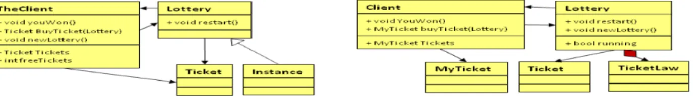
4.1.1 Running Example . . . 70
4.1.2 Minimalist Model for Diagram Representation . . . 70
4.1.3 Diagram matching within an ETGM framework . . . 72
4.1.3.1 Integrating lexical information . . . 72
4.1.3.2 From one-to-one to many-to-many matching . . . 73
4.1.4 Assigning costs to edit operations. . . 74
4.1.4.1 Basic cost parameters . . . 74
4.1.4.2 Assigning costs to merge operations . . . 76
4.1.4.3 Tuning the ETGM Cost Model . . . 77
4.2 MADMatch: A search based Many-to-many Approximate Diagram Matching approach . . . 79
4.2.1 Obvious matches and Filter I . . . 80
4.2.2 Getting the terms composing entities’ names . . . 82
4.2.3 ”Termal footprint” and Entity-Term Matrix (ETM) . . . 83
4.2.4 Entity ”Semilarity” and Filter II . . . 85
4.2.5 Entity similarity . . . 86
4.2.7 Application on the running example . . . 91
4.3 Empirical evaluation . . . 92
4.3.1 Research Questions . . . 92
4.3.2 Experimental plan for class diagrams . . . 93
4.3.2.1 Modeling and extraction . . . 93
4.3.2.2 Class diagram differencing . . . 95
4.3.2.3 API Evolution . . . 96
4.3.3 Experimental plan for sequence diagrams . . . 97
4.3.4 Experimental plan for Labeled Transition Systems (LTS) . . . 99
4.3.5 Analysis plan of the results . . . 102
4.3.5.1 Accuracy metrics and manual validation . . . 102
4.3.5.2 Devising scalability analysis . . . 106
4.3.5.3 Devising genericness analysis . . . 106
4.3.6 Experimental settings . . . 107
4.4 Evaluation results . . . 107
4.4.1 RQ1 – Accuracy of the returned solutions . . . 108
4.4.1.1 Class Diagram Differencing . . . 108
4.4.1.2 API Evolution . . . 111
4.4.2 RQ2 – MADMatch Scalability . . . 111
4.4.3 RQ3 – MADMatch Genericness . . . 112
4.4.3.1 Results on sequence diagrams . . . 114
4.4.3.2 Results on Labeled Transition Systems . . . 117
4.5 Discussion . . . 119
4.5.1 Summary . . . 119
4.5.2 Qualitative analysis of the DNSJava case study . . . 119
4.5.2.1 Class/package evolution . . . 120
4.5.2.2 Method/Attribute Level . . . 123
4.5.3 Challenges for matching techniques . . . 124
4.5.3.1 Challenging situations . . . 124
4.5.4 Considerations about entity evolution . . . 128
4.5.4.1 Top-Down changes . . . 128
4.5.4.2 Transversal changes . . . 129
4.6 Conclusion . . . 129
CHAPTER 5 DESIGN EVOLUTION METRICS FOR DEFECT PREDICTION . . . 131
5.1.1 Definitions . . . 133 5.2 Case Study . . . 134 5.2.1 Objects . . . 135 5.2.2 Treatments . . . 136 5.2.3 Research Questions . . . 136 5.2.4 Analysis Method . . . 137
5.2.5 Building and Assessing Predictors . . . 139
5.3 Results and Discussion . . . 141
5.3.1 RQ1 – Metrics Relevance . . . 141
5.3.1.1 Most Used Metrics . . . 141
5.3.1.2 Proportion of variability explained . . . 141
5.3.2 RQ2 – Defect-proneness Accuracy . . . 143
5.3.2.1 Most Used Metrics . . . 143
5.3.2.2 Analysis of the Obtained Means . . . 145
5.3.2.3 Wilcoxon Tests . . . 145
5.3.2.4 Cohen-d Statistics . . . 146
5.3.3 RQ3 – Defect count prediction . . . 147
5.3.3.1 Most Used Metrics . . . 147
5.3.3.2 Analysis of the Obtained Means . . . 149
5.3.3.3 Wilcoxon Tests . . . 149
5.3.3.4 Cohen-d Statistics . . . 150
5.3.4 RQ4 – Defect Density Prediction . . . 151
5.3.4.1 Most Used Metrics . . . 152
5.3.4.2 Analysis of the Obtained Means . . . 152
5.3.4.3 Wilcoxon Tests . . . 154 5.3.4.4 Cohen-d Statistics . . . 155 5.4 Threats to Validity . . . 156 5.5 Conclusion . . . 158 CHAPTER 6 CONCLUSION . . . 160 6.1 Synthesis . . . 160
6.1.1 Approximate Graph Matching . . . 161
6.1.2 Approximate Diagram Matching in software engineering . . . 163
6.1.3 Design Evolution Metrics for Defect Prediction . . . 163
6.2 Limitations . . . 164
6.3.1 Improving the algorithms . . . 165
6.3.2 Hybrid diagram matching approach . . . 166
6.3.3 Performing more experiments . . . 166
6.3.4 Software evolution . . . 167
LIST OF TABLES
Table 1.1 Complexity classes . . . 5
Table 3.1 Percentage of good node matches in top 5% similar (S3D2) node matches. 51 Table 3.2 Overview of our experiments and algorithms parameters . . . 56
Table 3.3 MCPS results on directed graphs with labels on both edges and nodes (score in percentage of the µ0 score) . . . 58
Table 3.4 MCPS results on directed graphs with labels on nodes (score in per-centage of the µ0 score) . . . 59
Table 3.5 MCPS results on directed graphs with labels on edges (score in per-centage of the µ0 score) . . . 59
Table 3.6 MCPS results on Directed, Unlabeled graphs (score in percentage of the µ0 score) . . . 60
Table 3.7 MCPS results on Undirected, Unlabeled graphs (score in percentage of the µ0 score) . . . 61
Table 3.8 Computation Times (in seconds) . . . 62
Table 3.9 MCPS results on Small, Directed graphs (score and computation time) 63 Table 3.10 MCPS results on Small, Undirected graphs (score and computation time) 64 Table 3.11 MCPS results on large graphs (n=3000, d=6, q=0.8) . . . 64
Table 3.12 MCPS results on dense graphs (n=300, d=60, q=0.8) . . . 64
Table 3.13 f1,1 results on Directed graphs (score and computation time) . . . 65
Table 4.1 ETGM cost parameters . . . 76
Table 4.2 ETGM Aggregate parameters . . . 78
Table 4.3 Terms in the example – number of occurrences are in brackets . . . 83
Table 4.4 Valid pairs of the running example after Filter II . . . 87
Table 4.5 LCS between terms of setLabelDrawnVerticla and drawVerticalLabel . 88 Table 4.6 Modeling class diagrams . . . 95
Table 4.7 Class diagram differencing: summary of the object systems (MAD-Match vs. UMLDiff) . . . 96
Table 4.8 API Evolution: summary of the object systems (MADMatch versus AURA) . . . 97
Table 4.9 Modeling sequence diagrams . . . 98
Table 4.10 Modeling labeled transition systems . . . 99
Table 4.11 MADMatch versus AURA (incorrect matches are in brackets, pA=pAgreement, dP=dPrecision, dR=dRecall) . . . 111
Table 4.12 Matching Specification to Markov model . . . 118
Table 4.13 Matching Specification to EDSM model . . . 118
Table 4.14 Refactorings found on DNSJava at the package and class level . . . 121
Table 4.15 Accuracy of different techniques for class-level operations on DNSJava (N/A indicates operations out of the scope of ADM’04) . . . 121
Table 4.16 DNSJava: A selection of change patterns occurring on methods . . . . 125
Table 4.17 DNSJava: A selection of change patterns occurring on attributes . . . . 125
Table 4.18 A selection of renaming patterns . . . 126
Table 5.1 Summary of the object systems . . . 134
Table 5.2 RQ1: Metrics kept 75% (or more) times when building linear regression models to explain the number of defects—TM = C&K for Rhino and ArgoUML, TM = Z&Z for Eclipse . . . 142
Table 5.3 Adjusted R2 from linear regressions on Rhino . . . 142
Table 5.4 Adjusted R2 from linear regressions on ArgoUML . . . 144
Table 5.5 Adjusted R2 from linear regressions on Eclipse . . . 144
Table 5.6 RQ2: Metrics kept 75% (or more) times when building logistic regres-sion models to predict defective classes—TM = C&K for Rhino and ArgoUML, TM = Z&Z for Eclipse . . . 145
Table 5.7 C&K+DEM ≤ C&K? p-value of Wilcoxon signed rank test for the F-measure of defective classes (confidence level: light grey 90%, dark grey 95%) . . . 146
Table 5.8 C&K+DEM ≤ random? p-value of Wilcoxon signed rank test for the F-measure of defective classes (confidence level: 95%) . . . 147
Table 5.9 Assessing C&K+DEM improvement over C&K: Cohen-d statistics (per-centage of defective classes) . . . 148
Table 5.10 Assessing C&K+DEM improvement over random: Cohen-d statistics (percentage of defective classes) . . . 148
Table 5.11 RQ3: Metrics kept 75% (or more) times when building Poisson regres-sion models to predict the number of defects—TM = C&K for Rhino and ArgoUML, TM = Z&Z for Eclipse . . . 148
Table 5.12 C&K+DEM ≤ C&K? p-value of Wilcoxon signed rank test for the percentage of defects per top classes (confidence level: light grey 90%, dark grey 95%) . . . 150
Table 5.13 C&K+DEM ≤ random? p-value of Wilcoxon signed rank test for the percentage of defects per top classes (confidence level: 95%) . . . 151
Table 5.14 Assessing C&K+DEM improvement over C&K: Cohen-d statistics (per-centage of defects) . . . 152 Table 5.15 Assessing C&K+DEM improvement over random: Cohen-d statistics
(percentage of defects) . . . 153 Table 5.16 RQ4: Metrics kept 75% (or more) times when building Poisson
re-gression models with different metric sets—TM = C&K for Rhino and ArgoUML, TM = Z&Z for Eclipse . . . 153 Table 5.17 DEM ≤ C&K? p-value of Wilcoxon signed rank test for the percentage
of defects per top LOCs (confidence level: light grey 90%, dark grey 95%) . . . 154 Table 5.18 DEM ≤ random? p-value of Wilcoxon signed rank test for the
percent-age of defects per top LOCs (confidence level: 95%) . . . 155 Table 5.19 Assessing DEM improvement over C&K: Cohen-d statistics (defect
den-sity) . . . 156 Table 5.20 Assessing DEM improvement over random: Cohen-d statistics (defect
LIST OF FIGURES
Figure 1.1 Types of graphs . . . 3
Figure 1.2 Search space, local and global optimum . . . 7
Figure 2.1 Main Graph Matching Formulations . . . 13
Figure 2.2 Main Families of Algorithms used for Graph Matching . . . 17
Figure 3.1 Modeling of the MCPS and the f1,1 problems . . . 35
Figure 3.2 Generation of a pair of random unlabeled graphs with controlled dis-tortion . . . 38
Figure 3.3 Devising enhanced node similarity measures for graph matching . . . . 44
Figure 3.4 Simple example of graph matching . . . 45
Figure 3.5 Precision of prediction in top 5% candidates on all directed graphs . . . 52
Figure 3.6 SIM-T: A similarity enhanced tabu search . . . 54
Figure 3.7 Results on all directed graphs (Average score in percentage of the µ0 score) . . . 58
Figure 4.1 Example of class diagrams to be matched . . . 70
Figure 4.2 Simple Meta-Model for software diagrams . . . 71
Figure 4.3 Modeling of the running example . . . 72
Figure 4.4 Merges . . . 74
Figure 4.5 Block diagram of the MADMatch algorithm . . . 81
Figure 4.6 Samples from the entity-term matrices of the running example . . . 84
Figure 4.7 Samples from the entity-term matrices of the running example . . . 85
Figure 4.8 Possible Moves . . . 91
Figure 4.9 MADMatch Evaluation approach . . . 94
Figure 4.10 InserireEnteEmettitore EasyCoin1.2 . . . 100
Figure 4.11 InserireEnteEmettitore EasyCoin2.0 . . . 100
Figure 4.12 ModificareEnteEmettitore EasyCoin1.2 . . . 101
Figure 4.13 Labeled Transition System S . . . 103
Figure 4.14 Labeled Transition System M . . . 103
Figure 4.15 Labeled Transition System E . . . 104
Figure 4.16 Sample from an output file of MADMatch . . . 106
Figure 4.17 Boxplots of the compared accuracy measures from MADMatch versus UMLDiff . . . 109
Figure 4.18 Computation times for DNSJava, JFreeChart and ArgoUML . . . 113
Figure 4.20 Matching InserireEnteEmettitore1.2 to ModificareEnteEmettitore1.2 . . 116
Figure 5.1 Average F-measure for defective classes on Rhino per top classes . . . . 146
Figure 5.2 Average F-measure for defective classes on ArgoUML per top classes . 147 Figure 5.3 Average F-measure for defective classes on Eclipse per top classes . . . 149
Figure 5.4 Average Percentage of defects on Rhino per top classes . . . 150
Figure 5.5 Average Percentage of defects on ArgoUML per top classes . . . 151
Figure 5.6 Average Percentage of defects on Eclipse per top classes . . . 152
Figure 5.7 Average Percentage of defects on Rhino per top LOCs . . . 154
Figure 5.8 Average Percentage of defects on ArgoUML per top LOCs . . . 155
Figure 5.9 Average Percentage of defects on Eclipse per top LOCs . . . 156
Figure 6.1 From graph matching to defect prediction: Summary and publications . 161 Figure 6.2 Synthesis of the AGM algorithms SIM-T and MADMatch . . . 162
CHAPTER 1
INTRODUCTION
The work presented in this thesis aims essentially to propose a generic approach for the automatic processing of matching (or conversely differencing) tasks in software engineering. Such matching tasks are diverse but they typically involve software artifacts represented as diagrams. Those diagrams can be thought of as graphs given that they consist of entities linked together by relations. Graph matching appears then as the natural paradigm able to address those problems in a generic way. In particular, considering that artifacts to be matched are not necessarily identical, it is of interest to select a kind of graph matching which allows some flexibility about paired elements. Approximate graph matching fulfills this requirement in the sense that matched elements do not have to present the exact same information. However, the available body of work in this domain does not permit a straight adaptation from existing generic purpose algorithms. Original contributions to approximate graph matching are thus needed in order to effectively achieve the goals outlined above. In short, approximate graph matching techniques, their application on software diagrams and the insights gained from a software quality perspective constitute the main topics of this research document.
In the following sections, we first present some basic notions and concepts used throughout this document and introduce in more detail the context and motivation of our research. We then formulate our research problems and objectives before concluding with the presentation of the organization of the rest of this document.
1.1 Basic notions and concepts
In order to ease the reading of this document, we introduce some basic notions from graph and computational complexity theory.
1.1.1 Elements from Graph Theory
Graph theory (Berge (1958)) is a field of mathematics and computer science which focuses on the study of graphs and related problems. The mathematical structures referred to as graphs
1 represent a very powerful tool able to model a very large range of – natural or human-made
– objects or problems. They are thus among the most common representations of structures
1
and are notably used for networks, molecules, images etc. The relevance of graph theory in so many applied sciences contributes to the emergence of a large, specialized (and occasionally ambiguous) vocabulary associated to graphs. In the following subsections, we present basic notions about graphs which are relevant to the present thesis.
Informally, a graph can be described as a collection of objects (called nodes, vertices or points) possibly connected by pairwise relations (called edges or lines). This general definition is the basis for different models and generates many variants. The most common distinction is between directed and undirected graphs: in directed graphs (or digraphs), relations (thus called arcs, directed edges or arrows) linking two nodes are oriented and represented as ordered pairs of nodes. Other important types of graphs include: multi-graphs (also called pseudo-graphs) in which pairs of vertices can be connected by more than one edge, weighted graphs in which a weight (usually a real number) is associated with every edge (or node) and labeled graphs in which labels (usually strings) are attached to the edges and nodes. In addition, research literature sometimes refers to attributed graphs which can be viewed as a generalization of labeled and weighted graphs in the sense that many attributes (of possibly different types) can be attached to a single node or edge. Figure 1.1 presents examples for each of the above mentioned types of graphs.
A graph G is usually represented as a couple (V, E) where V is the set of the vertices and E the set of edges. The cardinality of the set V (the number of vertices) is referred to as the order of the graph while the cardinality of E (the number of edges) is the size 2. Given
a vertex v, its degree (or valence) is the number of edges incident to v and denoted deg(v). In directed graphs, one usually distinguishes between the number of arcs originating from a vertex v (out-degree of v) and the number of arcs which destination is v (in-degree of v). Similarly, considering the neighbors of a given node v (i.e. the nodes with an arc going to or coming from v), one may distinguish between in-neighbors (nodes with an arc going to v) and out-neighbors (nodes with an arc coming from v). Additionally, to each graph can be associated a measure of density which expresses the ratio of the number of edges and the number of possible edges; a graph with a relatively low density will be said sparse.
Although graphs can be defined using sets, they are more complex structures and many simple definitions on sets are less trivial when it comes to graphs. This is the case for the definition of a subgraph. Given a graph G = (V, E), a subgraph GS = (VS, ES) of G will
certainly satisfy the constraints VS ⊆ V and ES ⊆ E but those are not the only ones. The
graph obtained by considering a subset H of V and all the edges existing between two of its vertices is G(H), the subgraph of G induced by H. Alternatively, the same subset H may correspond to a partial subgraph of G if it contains only part of the edges existing between
2
two vertices of H.
Once two objects or problems have been represented as graphs, determining whether they are equal is not a trivial task and corresponds to the graph isomorphism problem (Miller (1979)). This well-known problem of graph theory equates to finding a bijection between the vertex sets of the two graphs which preserves information about the edges and vertices. In most cases, this bijection simply does not exist and a more general question is then to determine how much (quantitatively and qualitatively) two given graphs are similar: do they share common parts? If so, in what extent and at which level of detail?
1.1.2 Hard problems and Meta-Heuristics Difficulty of Computational problems.
Computational problems can be defined as generic requests over a set of (generally) infinite collection of objects, called instances. A first classification of those problems is based on the type of request made by a given problem. For instance, one may distinguish between decision problems (requiring yes or no answers for every instance) and optimisation problems (where the goal is to find a solution optimizing a given function). However, given that other kinds of problems (including optimisation problems) can be reformulated as decision problems, research in computability theory has typically focused on decision problems. Thus, a more important distinction is often made between decidable and undecidable problems. Decidable problems are those for which there exists an algorithm able to solve them. Here, an algorithm can be defined as a finite sequence of instructions which finishes and produces a correct answer for every instance of a problem.
In general, the performance of an algorithm is assessed by considering its use of compu-tational resources such as storage (memory use) and especially time. For a given algorithm, the concept of time complexity refers to the number of elementary operations which might be needed to process problem instances of arbitrarily large size. Based on their growth rates, algorithms will be roughly classified (in decreasing order of run-time efficiency) as either polynomial (O(nc), c ∈ R), exponential (O(cn), c > 1) or factorial (O(n!)) 3. Furthermore,
in theoretical computer science, an algorithm’s complexity depends on the mathematical model used to represent a general computing machine. Two main (equivalent) models of a Turing (Turing (1937)) machine (TM) are usually considered: deterministic TM and non-deterministic TM. In essence, from any given state, a non-deterministic TM uses a fixed set of rules to determine its future actions while a non-deterministic TM may have multiple possible future actions, with any of those multiple paths potentially leading to a solution.
The inherent level of difficulty of a problem is assessed using complexity classes derived
3
from the consideration of all the possible algorithms which could be used to solve the con-sidered problem. Depending on the time complexity and the type of TM concon-sidered, one can distinguish four main complexity classes for decision problems, as presented in Table 1.1.
Exponential time complexity problems (EXPTIME, NEXPTIME ) are considered as hard
4 and are intractable (due to combinatorial explosion) for all instances but those with the
smallest input size. In contrast, the complexity class P is generally perceived as the class of problems admitting efficient (i.e. polynomial) algorithms. As for the class NP, it represents the set of decision problems admitting efficiently (i.e. in polynomial time by a deterministic Turing machine) verifiable proofs that the answer is indeed yes. For function problems, this means that one can verify in polynomial time that a given solution is indeed a correct one. NP includes P but whether P equals NP (i.e. N P ⊂ P ) is still an open question (Cook (1971)) and one of the main unsolved problems in mathematics 5. The complexity class NP
also includes the set of NP-complete (NPC) decision problems (Garey and Johnson (1979a)) which can be informally presented as the hardest problems in NP. A problem proven to be NP-complete is generally considered as one for which a polynomial algorithm does not exist (if P 6= N P ). Another important complexity class often associated to NP (though not included in NP ) is the NP-hard complexity class which represent computational problems (including problems other than decision problems) ”at least as hard as the hardest problems in NP”.
Given that there are no known polynomial algorithms able to solve optimally NP-hard or NP-complete problems, there is interest in algorithms proposing good solutions at reasonable times.
Meta-Heuristics.
Meta-Heuristics (Glover and Kochenberger (2003)) represent a family of techniques often used to address hard problems. Although they do not guarantee optimal solutions, their high adaptability and their ability to search very large spaces of solutions explains their popularity for many combinatorial optimization problems: from graph coloring (Galinier and Hao (1999)) to the Traveling Salesman Problem (Lin and Kernighan (1973)). In particular, the TSP is a well-known combinatorial optimization problem formulated as follows: ”Given a list of cities and their pairwise distances, the task is to find a shortest possible tour that
4
Note that EXPTIME actually contains P and NP.
5
http://www.claymath.org/millennium/
Table 1.1 Complexity classes
Deterministic Turing machine Non-Deterministic Turing machine
Polynomial P NP
visits each city exactly once”. It will be used in the following to illustrate main ideas behind meta-heuristics.
Meta-heuristics usually try to optimize an objective function and proceed by using three main resolution strategies:
1. Constructive heuristics: the algorithm builds a solution from an initially empty config-uration (e.g. greedy algorithms)
2. Local search: A complete solution is iteratively modified (e.g. hill climbing, simulated annealing, tabu search)
3. Evolutionary search: A population of solutions is evolved through genetic operators such as selection, crossover, mutation (e.g. genetic algorithms)
Greedy algorithms (Cormen et al. (1990)) build a solution based on the maximization at each iteration of a greedy criterion (which may use information other than the objective function). For instance, with respect to the TSP, a well-known greedy algorithm is the Nearest-Neighbor (NN) algorithm which selects as the next city to visit, the nearest unvisited one. Greedy algorithms are usually very fast and can provide good solutions but for some problem instances, they are susceptible to return very bad solutions (Gutin et al. (2002)).
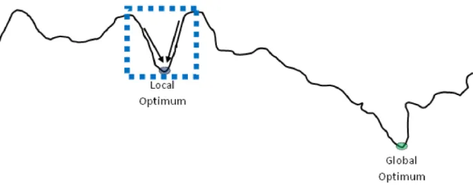
Local search algorithms define neighborhoods for solutions through possible moves from one solution to another, with the purpose of gradually moving solutions toward areas opti-mizing the objective function. For instance, from a given solution of the TSP (a tour that visits each city exactly once), a possible move is to permute the order in which two cities are visited. Ideally, from any given solution, the best possible moves would improve the objective function up to the point where the optimum is reached. In practice, a local search can get stuck in local optima: all neighboring solutions are worse than a given solution lO
(a local optimum) but there are better solutions than lO in other search areas, as illustrated
in Figure 1.2. Hill-Climbing (the simplest local search algorithm) is very vulnerable to this kind of scenarii because it does not permit a degradation of the objective function.
More sophisticated local search algorithms such as tabu search (proposed by Glover (1989)) and simulated annealing (Kirkpatrick et al. (1983)) propose additional mechanisms to escape local optima. In essence, a tabu search will forbid, through the use of (so-called) tabu lists, that the local search returns to areas recently visited. Usually, the mechanism does not explicitly forbid entire solutions but will rather try to prevent that moves recently made are rapidly (in terms of subsequent iterations) undone. Clearly, doing and undoing the same moves in a limited number of iterations can be harmful to the search process; the tabu search is designed to prevent this kind of situation. In the example proposed in 1.2, the tabu
Figure 1.2 Search space, local and global optimum
mechanism may allow the search to get away from the local optima by constantly forbidding the return to the local optimum area.
As for simulated annealing (Kirkpatrick et al. (1983)), it is inspired from a metallurgy technique (annealing) which uses the controlled cooling of a material as a way to reduce its defects. Each iteration, a random move mv is selected; if it improves the current solution, it is always accepted, otherwise whether mv is accepted or not depends on a probability computed using a cooling parameter T (the temperature) and the extent of the degradation brought by mv. At the beginning, the temperature T, initially high, is gradually lowered along with the probability of accepting moves degrading the solution. In the example proposed in 1.2, a simulated annealing may escape from the local optima by allowing moves which degrade the objective function.
Note that, unlike hill-climbing which usually stops when it reaches an optimum (either local or global), more complex local search algorithms need stop criteria. Those criteria can be based on a given number of iterations (possibly consecutive iterations without improvements of the objective function), the computation time, or even algorithm-specific parameters (such as the final temperature in simulated annealing).
Genetic algorithms (Holland (1975)), inspired from the evolutionary theory of Darwin, manage the evolution of a population (of solutions) toward the breeding of the fittest indi-vidual (with respect to the objective function). To achieve this goal, genetic operators (such as selection, crossover, and mutation) and principles (such as the survival of the fittest, etc.) are applied from generation to generation. At each generation, the best-fit individuals of the current population are selected for reproduction and generate offspring through crossover
and mutation operators. In general, the number of individuals is kept constant and thus, the least-fit individuals do not make it to the next generation.
Meta-heuristics define generic frameworks which should be enhanced by information spe-cific to the problems at hand. It is strongly recommended that greedy criterion, neighborhood definition, genetic operators etc. should all leverage a deep understanding of the problem being addressed (Wolpert and Macready (1997)).
1.2 Research context and motivation
Development of software applications involves much more than coding and every serious software project is expected to generate many by-products essential for its good completion quality and evolution. Consequently, most software projects involve the production of arti-facts which help describe their functionalities, architecture, design or implementation. The analysis of those by-products is particularly useful and fuels many important advances in soft-ware engineering as a discipline and profession. As softsoft-ware evolves, so do or should those by-products. Thus, comparing software artifacts is a recurrent task for which researchers and practitioners need efficient algorithms and tools. More specifically, given two objects gener-ated by software activities, there is often the need to retrieve the similarities and differences between them. A considerable amount of research has been devoted to address this issue from the perspective of a specific problem or artifact but very few work have tried to define and tackle an underlying and more general ”comparison problem”. This matter of facts may prevent or hinder progress on many interesting (well-established or emerging) software engi-neering sub-fields because part of the research effort could have to be diverted in developing custom-made algorithms for specific artifact comparison.
In practice, comparing two software artifacts equates to determine the changes (or dif-ferences) between them. Indeed, software engineering literature contains many approaches for the differencing (”diff-ing”) of an artifact. Most of the proposed algorithms actually pro-ceed as follows: ”match elements and infer the changes” to put it simply. Matching elements and/or sub-parts of considered artifacts is thus the core of most proposals and the work involved beyond this step is mostly trivial. Additionally, most of the software artifacts are (or can be represented as) diagrams and those diagrams are essentially graphs with richer information attached to nodes and edges. A generic and comprehensive approach applicable on graphs could then be an interesting option permitting to deal efficiently with the various matching problems identifiable in software engineering.
Graph matching refers to a set of problems involving the comparison of two graphs. It is often divided in two classes: exact graph matching and approximate graph matching
(also referred to as inexact graph matching). Exact graph matching includes well-known problems of graph theory such as graph isomorphism but it imposes a strict correspondence on nodes and relations to be matched. This is not practical in most real-life applications, including matching tasks in software engineering, where matchings of interest should tolerate errors of correspondence. On one hand, approximate graph matching offers that flexibility along with some elegant ways of modeling differencing problems. On the other hand, a review of algorithms addressing approximate graph matching reveal that (i) the vast majority of proposed approaches are very application-oriented and (ii) their target graphs do not necessarily look like the kind of graphs and diagrams found in software engineering. In fact, the (sometimes very specific) target graphs used in the evaluation of most techniques originate from a few research communities such as those of image processing, computer vision and bio-chemistry. As a result, researchers and practitioners from many fields, when facing an approximate graph matching problem, can be hard-pressed in choosing between algorithms (designed for other specific applications) and risk ending up with their choice being unable to scale up to the size of their own target graphs. Ultimately, this explains in part the lack of a unified framework for the resolution of matching tasks in software engineering and prompts the need to design and evaluate a generic AGM approach on generic graphs.
1.3 Research problems and objectives
From the research context, it is clear that our research problem integrate elements from computer science, software engineering and graph theory. The problems we address are interconnected but present their own specificity and challenges as exposed below.
1.3.1 Approximate Graph Matching
Determining the extent of similarity between two objects or problems represented as graphs is a recurrent and important question. Given two graphs, an intuitive answer consists in matching, with respect to some constraints, nodes and arcs from the first graph to nodes and arcs from the second. In many domains, the generated or observed graphs are subject to all kinds of distortions or modifications. There is thus, a needed flexibility about the constraints imposed on the matched elements. Such flexibility is typically introduced through mechanisms of bonus and/or malus: matching two elements may result in either a gain or a loss depending on how similar they are. The sought solution is then the one which maximizes the gains and/or minimizes the losses. This general schema is translated into many different formulations but they share a common characteristic: their NP-hardness. This means (if P 6= N P ) that polynomial algorithms cannot guarantee to solve them optimally. Most
of the relevant literature on AGM propose many interesting techniques addressing a given formulation. However, there are also important work aiming to propose common framework and formulation able to integrate most of the specific variants. Those frameworks provide the basis of the investigation for a generic AGM technique which can be effective and efficient for most formulations and target graphs.
Our first research objective is thus formulated as follows: Propose an approximate graph matching approach readily usable on (or easily adaptable to) matching problems arising in many real-life applications. Consequently, our focus is on graphs stripped of specificities encountered in given fields and the goal is to develop efficient techniques making the best use of the minimal information one can retrieve on every graph: structural information.
1.3.2 Diagram Matching in Software Engineering
Identifying the commonalities and differences between two diagrams is an important task in software engineering, especially in software evolution analysis. Accurate information about the history of (or subsequent changes occurring on) a given artifact or entity is much needed in many applications such as project planning or defect prediction. Although graph matching can be used as a robust framework to address those activities, (software) diagrams have some specificities which should be integrated in order to have efficient algorithms. In particular, in contrast with the graphs that we address in the first research objective, textual information is in this context as important as structural information, prompting the need to explore textual similarity comparison and asking the question of the weighting of structural and textual information.
Our second research objective is thus formulated as follows: Propose a generic and scalable approach for the automatic processing of diagram comparison problems arising in software engineering.
1.3.3 Evolution metrics for Defect prediction
There are a number of insights one can get from the comparison of software artifacts. In particular, in a software evolution context, there are many valuable information one can get from the evolution profile of a given entity. Once changes occurring on entities are retrieved, software engineers and testers may be interested in inferring directly useful knowledge about the system being developed.
Defect prediction has been one of the most active research lines with direct practical use for the industry. The potential of this research is enormous: if it becomes possible to predict the location and/or number of bugs in specific modules, savings in terms of testing effort
would be substantial. The problem has been tackled from a number of perspectives, from sampling techniques to machine learning models but the main input are metrics which are proposed and supposed to correlate with defect occurrences. The relation between changes and defects is an established one but there was no work investigating the effect of hi-level changes on the defect proneness of source code.
Consequently, our third research objective is to propose evolution metrics able to predict defect location.
1.4 Thesis plan
The rest of this document is organized as follows. Chapter 2 reviews three research areas related to our work, i.e., graph matching, differencing software artifacts and defect prediction. Chapter 3 presents our approach on approximate graph matching. Our proposal is a tabu search initialized using adequate structural similarity measures. Chapter 4 presents the adaptation and application of our graph matching framework on software diagrams and discuss some of our findings. In Chapter 5, we define simple design evolution metrics for object-oriented systems and investigate their use for defect prediction. Finally, Chapter 6 summarizes our work and outlines possible future directions.
CHAPTER 2
RELATED WORK
The current chapter is devoted to the review of the three main research areas relevant to the work presented in this thesis. In the following, we first review graph matching literature (the different formulations and techniques) then present an overview of differencing approaches in software evolution before ending with related work on defect prediction.
2.1 Graph matching in research literature
Graph representations are among the most common and effective ways to model all kinds of natural or human-made objects. Once two objects or problems have been represented as graphs, their comparison is a fundamental question in many different applications and is referred to as graph matching.
Research work on graph matching is very active and multi-disciplinary as graphs to be matched can represent images (Toshev et al. (2007)), molecules (Wang et al. (2004)), soft-ware artifacts (Abi-Antoun et al. (2008)) etc. Formulations of the problem and proposed algorithms are manifold. The body of work is so large and diverse that, reminiscent of what can be observed for graphs, the vocabulary associated to graph matching is very extended and sometimes ambiguous.The goal of the current section is to present a concise picture of the state-of-the-art in graph matching. In the following, we first present the most important formulations of graph matching and the main families of techniques used for these problems. We then discuss the way the evaluation of the proposed techniques is conducted, in particu-lar the benchmarks used and conclude by highlighting the lessons learned and the intuitions confirmed from the review of graph matching literature.
2.1.1 Graph Matching formulations
Graph matching is a generic term which corresponds in fact to many different specialized formulations which can be regrouped in two main categories: exact graph matching and approximate graph matching 1. Figure 2.1 previews the most important formulations of
graph matching, the ones which will be detailed in the following.
1
Figure 2.1 Main Graph Matching Formulations
2.1.1.1 Exact Graph Matching
Graph matching problems of this category do not tolerate differences between matched nodes and edges. They abide to the edge-preservation constraint which requires that edges con-necting two matched nodes must be perfectly matched. The main problems of this category are Graph Isomorphism (Miller (1979)) and Induced Subgraph Isomorphism (Cook (1971)) but there exist other interesting formulations.
Graph Isomorphism (GI) Given two graphs G1 = (V1, E1) and G2 = (V2, E2), with
|V1| = |V2|, the problem consists in determining whether there exists a bijective one-to-one
mapping f : V1 → V2 such that (x1, y1) ∈ E1 ⇔ (f (x1), f (y1)) ∈ E2. In the general
case, when some kind of information (labels, weights, attributes) is attached to the ver-tices and edges, appropriate formulations will usually require the preservation of that in-formation: inf ormation(x1) = inf ormation(f (x1)) ∀x1 ∈ V1 and inf ormation(x1, y1) =
inf ormation(f (x1), f (y1)) ∀(x1, y1) ∈ V1× V1. When such a mapping f exists, G1 is said to
be isomorphic to G2. In most problem instances, the strong constraints described above and
their implications (for instance, only vertices of the same degree can be matched) will reduce drastically the mapping possibilities and ease the discovery of a bijective mapping. However, in the general case, it is still unclear whether polynomial algorithms can solve optimally the GI problem.
Induced Subgraph Isomorphism Given two graphs G1 = (V1, E1) and G2 = (V2, E2),
between the smallest graph (G1) and an induced subgraph SG2 of the biggest graph (G2).
The problem is known to be NP-complete.
Exact Subgraph Matching Matching two given graphs equates to mapping their sub-parts: nodes, edges and arguably subgraphs. There can be some ambiguity in the adopted subgraph definition. In our view, one can talk about exact graph matching only if the sub-graphs induced by the matched vertices are isomorphic. In that sense, the maximum common subgraph (MCS) problem in which the goal is to find the largest (in terms of the number of vertices or edges) common subgraph of two graphs can be classified only if precision is brought on which kind of subgraph is sought. If one is seeking common induced subgraphs, it corresponds to the maximum common induced subgraph (MCIS) 2 problem (Garey and
Johnson (1979b)) which can be classified as an exact graph matching problem. Note that the MCIS problem is known to be NP-hard and can be used to model Graph Isomorphism and Induced Subgraph Isomorphism.
Reformulation as a maximum clique problem A common way to tackle exact graph matching is through the reformulation as another well known and studied problem of graph theory: the maximum clique problem (Haris et al. (1999); Raymond et al. (2002)). Given an undirected graph G = (V, E), a clique is a subset C of V such that there exists an edge connecting every two vertices of C. A maximum clique is simply a clique of the largest possible size in a given graph. The link with graph matching is made by considering a compatibility (or association) graph whose vertex set is included 3 in the cartesian product
of the vertex sets of the two graphs (G1 and G2) to be matched. Between each two vertices
(x1, x2) and (y1, y2) (with x1, y1 ∈ V1 and x2, y2 ∈ V2) of this compatibility graph, there
will be a link if the node matches are compatible: information linking (or not) x1 and y1 is
identical to information linking (or not) x2 and y2. Retrieving the maximum clique in such a
graph equates to finding the maximum (relatively to the number of nodes) common induced subgraph between G1 and G2. Additional mechanisms (such as weights assigned to the nodes
or edges) can be used to find the biggest subgraph in terms of edges 4. The maximum clique
problem is known to be NP-hard (Karp (1972)).
2
also called Maximum Common Subgraph Isomorphism problem
3
The vertex set of a compatibility graph may exclude some pairs if information attached to them is not compatible.
4
It is even possible to keep the clique analogy for approximate graph matching, provided substantial adjustments.
2.1.1.2 Approximate Graph Matching
In most real-life scenarios, the information brought by exact graph matching formulations is not satisfactory. Their strict constraints, while potentially very helpful in algorithms, usually prevent the detection of common parts between two graphs. Consequently, more flexible graph matching formulations have been proposed, among which the Maximum Common Partial Subgraph (MCPS) problem (Raymond et al. (2002)), the Weighted Graph Match-ing (WGM) problem (Umeyama (1988)) and the Error-Tolerant Graph MatchMatch-ing (ETGM) problem (Sanfeliu and Fu (1983); Bunke (1998)).
Maximum Common Partial Subgraph (MCPS) The MCPS problem is among the simplest approximate graph matching formulations and it can serve as a good introduction to core ideas of approximate graph matching. Similar to the MCIS problem, it clearly refers to the optimization (maximization) of a certain criterion: usually, the number of perfectly matched edges5. And more importantly, it relaxes the edge-preserving constraint of exact
graph matching: given two nodes x1 and y1 from one graph and their matched counterparts
x2 and y2 from the other graph, information linking (or not) x1 and y1 is not required to be
identical to information linking (or not) x2 and y2. Exact correspondences will still be sought
as they will contribute to the objective function This formulation of Approximate Graph Matching is useful in many practical contexts (notably in bio-chemistry applications) but it is quite limited by the fact that its objective function is a simple count of perfect (edge) matches.
Weighted Graph Matching (WGM) The WGM problem (Umeyama (1988)) is a graph matching formulation which targets graphs with weights on their edges and aims to minimize the distance between the adjacency matrices of two given graphs. The original formulation assumes that the two graphs have the same size and a permutation matrix P can thus be used to encode a solution; Pij = 1 if vertex i of graph G1 is matched to vertex j of graph G2
and zero otherwise. Formally, the WGM problem is defined using a least-square formulation: minP∈Π||A1− PTA2P ||2F
where Π is the set of permutation matrices, A1 and A2 the adjacency matrices of the graphs
G1 and G2 and ||.||2 is the square of an euclidean norm. Node information can be exploited if
a dissimilarity function or matrix is provided for the nodes. The objective function can thus
5
When looking for a common partial subgraph, maximizing the number of vertices is a trivial problem. The number of edges is the only interesting option and this explains the occasional confusion of the MCPS problem with the Maximum Common Edge Subgraph (MCES) problem
integrate nodes and the optimal matching will contain not only edges with similar weights, but also vertices with similar labels. The objective function then becomes
minP∈Π(1 − α)||A1− PTA2P ||2F + αC T
PT
where C is a matrix encoding pairwise dissimilarities between vertex labels of two graphs, and α controls the trade-off between edge and vertex alignment components (the greater α, the more importance is given to matching vertices with similar labels). Furthermore, the WGM problem can be extended to graphs of different sizes through the introduction of dummy nodes. Unlike the MCPS, comparison of the graph elements (nodes and edges) does not result in a binary yes/no answer and this allows a more fine-grained comparison in the cases where information dissimilarity on the graph elements (nodes an edges) can be quantified. A severe limitation of this formulation is that the edges cannot have attributes other than their weight. Consequently, one can not explicitly forbid the matching of specific types of edges or even apply specific costs for specific edges.
Error Tolerant Graph Matching(ETGM) In this formulation (Sanfeliu and Fu (1983); Bunke (1998)), the matching cost of two graphs is based on an explicit model of the errors (distortions) that can occur (i.e. missing nodes, etc.) and the costs that they may trigger. This idea is often extended to the concept of graph edit operations: one defines a set of edit operations on graphs, each with an assigned cost, and the goal of the problem is to find a series of those operations (transforming the first graph into the second one) with a minimum cost. Those operations are typically deletions (corresponding to unmatched elements from the first graph), insertions (corresponding to unmatched elements from the second graph) and substitutions (occurring when elements are matched). Costs assigned to those operations inform about the desired matching and algorithms can be applied to find the cheapest sequence of operations needed to transform one of the two graphs into the other. Under certain constraints on the assigned costs, this edit cost can satisfy distance requirements (commutativity, etc.) and Error Tolerant Graph Matching is sometimes called the Graph Edit Distance (GED) problem. The ETGM problem is proven NP-hard (Bunke (1998)) and can be used to model other AGM formulations provided the right edit operations and associated costs.
2.1.2 Approximate Graph Matching Algorithms
Various kinds of techniques have been proposed to address the different formulations of graph matching problems. The line between formulations and techniques for Graph Matching is
Figure 2.2 Main Families of Algorithms used for Graph Matching
quite blurred, and many algorithms are only applicable for a given formulation or type of graph. Figure 2.2 presents the most important families of techniques used to address graph matching problems. We propose in the following a more detailed review (partially inspired by the classification of Conte et al. (2004)) of those techniques.
2.1.2.1 The Hungarian algorithm
The Hungarian method (Kuhn (1955)) 6 is an algorithm widely used in graph matching
problems. It solves optimally in polynomial time the assignment problem which consists in finding a maximum weight matching in a weighted bipartite graph. When used for graph matching, the vertex set of the bipartite graph is the union of the vertex sets of the two graphs to be matched; edges exist only between nodes of different graphs and are weighted with a node similarity value expressing the similarity (or the mapping cost) of the nodes in presence.
Node Similarity The similarity between nodes of two graphs is an important concept (not limited to its use by the Hungarian problem) in graph matching and certainly one of the most intuitive measures for assessing the quality of a given node match. Node similarity refers to
6
The name is an acknowledgment of the influence of earlier works of two Hungarian mathematicians: Denes Koenig and Jeno Egervary.