Rapport de recherche présenté à
M. Francisco Ruge-Murcia, directeur de recherche
Could the Asian Crisis Have Been More Accurately Predicted? Improving an Early Warning System Model
Par Sacha Des Rosiers DESS08617902
Université de Montréal Septembre 2006
TABLE OF CONTENTS
Abstract....………4
Section I. Introduction……….5
Section II. Early Warning Systems in the Light of the Asian Crisis………...7
2.1 The Asian Currency Crisis of 1997………...7
2.2 A Brief Definition of Early Warning Systems………...7
Section III. Review of the Literature on Early Warning Systems.………11
3.1 The Leading-Indicator Approach……….11
3.1.1 Kaminsky, Lizondo and Reinhart (1998)………..11
3.2 The Discrete-Dependent-Variable Approach………..13
3.2.1 Eichengreen, Rose and Wyplosz (1995)………...14
3.2.2 Frankel and Rose (1996)………...15
3.3 An Example of the Third Generation of Models……….17
3.3.1 Zhang (2001)……….17
Section IV. Theoretical Analysis………...20
4.1 Jacobs, Kuper and Lestano (2004)………...20
4.1.1 The Purpose of Factor Analysis………21
4.1.2 The Use of Logit Modeling………...21
4.2 Bussière and Fratzscher (2002)………22
4.3 The Hypothesis to Verify……….23
Section V. Empirical Analysis………...24
5.1 Part I: Setting Up the Data………...24
5.1.1 The Data………24
5.1.2 The Independent Variables………...24
5.1.3 Transformations of the Data……….25
5.2 Part II: Methodological Steps in Factor Analysis………26
5.2.1 A Brief Definition of Factor Analysis………..26
5.2.2 Step 1: Choosing the Matrix of Associations………...27
5.2.3 Step 2: Factor Extraction Procedure.………27
5.2.4 Step 3: The Rotation Method………...28
5.2.5 Step 4: Number of Factors to Extract………...29
5.3 Part III: Multinomial Logit Analysis………...30
5.3.1 Step 1: Computing an Index……….30
5.3.2 Step 2: Definition of a Crisis………31
5.3.3 Step 3: What the Model wants to Predict………..31
5.3.4 Interpretation of the Regimes………32
5.4 Results and Evaluation of the Performance of the Multinomial Logit Model using Factor Analysis………...33
5.4.1 The Signal-to-Noise Ratio as a Measure of Performance………….34
5.4.2 The Results obtained by Jacobs, Kuper and Lestano (2004)………35
5.4.3 The Results obtained by this Paper………...37
5.4.4 Evaluation of the Multinomial Logit Model………37
Section VI. Conclusion………..39
Section VII. References……….43
Section VIII. Appendix………..45
Table A1. Explanatory Variables: Definitions, Sources and Transformations…..45
ABSTRACT
The Asian crisis of 1997 took experts by surprise not only because of its suddenness but also because of its amplitude. The agents involved saw the urgency to monitor variables (namely indicators) that can affect the economic health of countries. One way of using these vulnerability indicators is to construct early warning systems (EWS). Their aim is to be able to trigger an alarm informing policymakers that the probability of a crisis is relatively high. In their paper, Jacobs, Kuper and Lestano (2004) present an econometric EWS in which, among other things, they combine factor analysis to binomial logit modeling for six Asian countries. Using this combination, they then measure performances of already existing crisis definitions in terms of their predictive powers. They conclude that the dating scheme developed by Kaminsky, Lizondo and Reinhart (1998) is superior to the other models. This present paper aims to improve these results by combining factor analysis with the dating scheme and most importantly the multinomial logit model proposed by Bussière and Fratzscher (2002). According to their conclusions, having more than two outcomes in a logit model increases its predictive power. Simply put, the following pages try to answer the question: Could the Asian crisis of 1997 have been predicted with more accuracy? The conclusions are mitigated. In general, combining factor analysis and multinomial logit modeling does not show better predictive powers than the ones calculated by Jacobs, Kuper and Lestano. Yet, it is not the worst of the models tested.
I. INTRODUCTION
Economic crises have been a phenomenon well documented and yet, agents involved have not been able to fully understand it, as it can still strike and leave in its furrow important social, political and economic costs. Indeed, the last decade has seen its share of financial turmoil: The Mexican “tequila effect” (1994), the Asian “flu” (1997), the Russian (1998) and the Brazilian crises (1999).
One of the main goals in taking interest in the phenomenon is to be able to prevent it. Foreseeing crises is the key for political leaders to take pre-emptive actions in order to avoid or lower economic turbulences. This paper will therefore emphasize on forecasting economic crisis and more specifically on the prediction of the Asian currency crisis of 1997.
Various avenues exist to tackle the issue of anticipating a crisis. The one that will be chosen in this paper refers to the existence of a monitoring tool, the early warning system or EWS. Like its name refers to, an EWS model has the task of giving signals that a crisis might occur. The data that such a model uses are called indicators. Changes in indicators trigger a signal.
In their paper Jacobs, Kuper and Lestano (2004) lean into the case of indicators by building an econometric early warning system for the six Asian countries the most affected in 1997. They first construct factors using a factor analysis methodology. The factors originate from a broad set of potentially relevant indicators of currency crisis taken from literature. The factors found are then used as indicators and put into a binomial logit model where crisis and non-crisis periods are the two outcomes. Their general conclusion states that some of the indicators do work for the six Asian countries. In other words, the combination of factor analysis and logit modeling adds to the predicting power of the early warning systems analysed in their paper.
A more specific task that the authors undertake is the comparison of different dating schemes. Defining dates of a crisis is at the core of building an EWS model: It differentiates one model from another. Using the combination of factor analysis and binomial logit modeling, the authors compare the performance of four models developed by Eichengreen, Rose and Wyplosz (1995), Frankel and Rose (1996), Kaminsky,
Lizondo and Reinhart (1998) and Zhang (2001), as well as versions of Kaminsky, Lizondo and Reinhart and Zhang modified by Jacobs, Kuper and Lestano.
To measure the performance of the different models, Jacobs, Kuper and Lestano use signal-to-noise ratios. Put simply, these ratios are calculated as the probabilities of right crisis predictions divided by the probabilities of wrong crisis predictions. A signal-to-noise ratio is then the tool that evaluates the predictive power of models hence permits to tell if a model is better (or more accurate) then another model. Their conclusion is that the model developed by Kaminsky, Lizondo and Reinhart (1998) performs better than all the other models.
The present paper aims to ameliorate the results of the Jacobs, Kuper and Lestano research. In order to achieve this, the same factors found by the authors will be inserted in the logit model proposed by Bussière and Fratzscher (2002). They conclude that their model significantly improves the predictive power of logit methodology because not only it proposes three outcomes instead of two, but it also presents a different crisis dating scheme. This discrete-dependant variable approach is then called a multinomial logit model.
In concrete terms, the aim of this present paper is to try to get higher signal-to-noise ratios than the ones calculated by Jacobs, Kuper and Lestano. Put in other terms, this paper attempts to answer the following question: Having combined factor analysis and multinomial logit modeling, could the Asian crisis have been predicted more accurately?
Before answering this question, some background information on early warning systems will be presented in section 2. It will be followed, in section 3, by a review of what has been achieved so far in the literature. Section 4 will expose the theoretical analysis surrounding the research question in which both researches of Jacobs, Kuper and Lestano and of Bussière and Fratzscher will be described thoroughly. Section 5 will present the empirical analysis that illustrates the steps to answer the question and will show results. Finally, a conclusion will be drawn in section 6.
II. EARLY WARNING SYSTEMS IN THE LIGHT OF THE ASIAN CRISIS
2.1 The Asian Currency Crisis of 1997
Prior to the crisis of 1997, the Asian countries were embarked in an irresistible boost depicted by a dynamic picking up of the industrialised economies. Japan, Honk Kong, South Korea, Singapore, Taiwan, Indonesia, Thailand and Malaysia had on average a growth rate twice as big as the average growth rate of industrialised countries, three times as big as the Latin American ones and five times as big as the Sub-Saharan African countries. According to experts, the Asian countries were becoming a unique emerging region where differences were being erased, so that a single path toward progress was being drawn.
Thus a known characteristic of the Asian crisis of 1997 is its element of surprise. The fact that it was unexpected perhaps aggravated its intensity and amplitude as contagion spread from Thailand to the rest of the Asian countries. Apart from Thailand the most affected countries were Indonesia, Malaysia, the Philippines, South Korea, and Singapore. It even touched China, Russia and Brazil a year later. In fact, international stock markets hit record lows because the volatility and the unpredictability of financial markets scared investors.
The architects monitoring financial international vulnerability learned two main lessons from the Asian episode. First, the high costs triggered by economic crises demonstrated the importance of monitoring early warning indicators. Secondly, the deficiency of the most closely watched market indicators was pointed out. Consequently the implementation of early warning systems as a monitoring tool for identifying financial vulnerability was encouraged.
2.2 A Brief Definition of Early Warning Systems
As the concept of early warning systems is relatively new in the field of economics, the reader may not be familiar with such notion. A quick overview of what has been done so far in the field may come in handy. The following paragraphs present a definition of early warning systems. Included in this definition are the advantages and the issues that researchers are now facing when using such tools. The section concludes by
examining the three main categories (or generations) that researches fall into when building early warning systems.
The definition of an early warning system model takes its sense in the aim that such model is attended for. Its objective is to be able to trigger a sort of red light informing economic agents that according to the data in hand, the probability that a crisis will occur is relatively high. The crisis could be a financial, banking or a currency crisis. Empirically speaking, an early warning system is composed of a specific definition of the crisis (in other words, the dating scheme of the crisis) as well as a device for generating prediction. It includes a set of variables that help to predict a crisis namely, indicators.
The purpose of this systematic method is then to distinguish stylized facts into periods that are a prelude to a crisis. Said differently, the model is devised to differentiate the behaviour of indicators before a crisis from their sustainable behaviour, in tranquil periods. Therefore, the expected strength of early warning system models is to foresee significant crisis threats that former methods of analysis do not depict. As Berg, Borensztein, Milesi-Ferretti and Pattillo mention (1999, p. 3): The main advantage of using early warning systems lies in the fact that
[…] they process the information contained in the rather large number of relevant variables in a systematic way that maximizes their ability to predict […] crises, based on the historical experience of a large number of countries. Often, an early warning system can translate this information into a composite measure of vulnerability. Being based on well-defined methodology, it is less likely to be clouded by preconceptions about the expected economic performance of particular countries.
In the meantime, a well-constructed EWS model should avoid a disproportionate number of false alarms that weakens the credibility of crisis signals.
Even if the attention of such tools grew rapidly in the last years, one should understand that research is still in its primary stages, as shown by certain issues that early warning system modeling faces. Indeed, how a researcher tackles these issues leads to the development of different models. The problematic subjects are the differences in the definition of crises (the dating scheme of a crisis), the time span, the methodology (or mechanism) to apply for generating predictions and the choice of variables to use as indicators. As up to now, there is still no consensus on the definition of crises and parallel
to this, no agreement on the design of the optimal method to predict crises. Thus, this addresses a number of practical and conceptual concerns. In fact, as the implementation of early warning systems is quite new, it is recognized that such tools are not precise enough to act as the exclusive method to foresee crises but is rather viewed as a tool embedded in the analysis of crisis prediction.
Nonetheless, it is established that early warning systems are helpful tools that demonstrate a potential for future research. That is why it is valuable to built early warning systems that are able to single out adequately the risk of experiencing a crisis. In that sense, the literature on early warning systems is quite rich.
Researches referring to early warning signal models are mainly classified under two broad categories also known as first and second generations. A third generation exists but it is the source of many disagreements amongst researchers.
The main postulate of the first-generation models is that there are inconsistent macroeconomic policies with the maintenance of a currency peg. This leads to speculative attacks that are then the result of rational speculation with perfect foresight, and not the consequence of a random speculative attitude. In other terms, first-generation models demonstrate that unsuitability of joined economic policies can initiate a deterioration of fundamentals. Consequently, it informs investors about potential risks, thus generating speculative attacks. The starting point of a crisis is then weak fundamentals, as stated by Krugman (1979) in his model of balance-of-payment crises.
On the other hand, the second-generation models have been built regarding the inability of the first-generation models to explain contemporaneous crises such as the European exchange rate mechanism collapse. Indeed, this episode reveals that countries that practise sensible policies compatible with maintaining a fixed exchange rate can still be victims of speculative attacks. Thus the second-generation models share the postulate that abrupt changes in views about maintaining sound macroeconomic politics are plausible. This leads to the existence of multiple equilibria (as opposed to the existence of a unique equilibrium in the first-generation models). The second-generation models
[…] were developed to demonstrate that a crisis could be caused by self-fulfilling speculative attacks rather than by deteriorating economic fundamentals […]. The models focus on the dynamic interactions of market expectations and the conflicting objectives of the government and show
how this can lead to a self-fulfilling run on domestic currency (Sharma, 2003, p. 179).
Having said that, the presence of self-fulfilling speculative attacks does not exclude the existence of weak fundamentals. On the contrary, fundamental and vulnerability indicators can play a complementary role when predicting crises, as pointed out by the third generation of models.
Indeed, a controversial third generation exists but the reader should keep in mind that any definition of what constitutes a third-generation model suffers from many criticisms as there is no general consensus to agree on one. Nonetheless, most researchers agree that the basis of any model within this category is to reconcile the first and second generations’ strengths. Moreover, many supporters of any of the two generations reach agreement in the fact that the perspective of a weakening economy rises the economy’s vulnerability to a crisis.
Krugman (1996), summarised in Sharma (2003), is one of the first economists who undertakes the task of combining the two categories: The new generation of models is
[…] retaining the more sophisticated behaviour of governments from the second generation models [and considers that] in most crises, fundamentals are not stable but are deteriorating or are expected to deteriorate because the current economic situation appears unsustainable (2003, p. 181).
Furthermore Sharma clarifies what should constitute a third-generation model: The third-generation models will have to emphasize on the relationship between financial sector weakness and the investor behaviour, including the effects of exogenous shocks to financial intermediaries that provide liquidity services. Moreover, it must illustrate how poor policy makes a country vulnerable to abrupt shifts in investor confidence, and how the sudden rise of investor expectations of a crisis can force a policy response that validates the original expectations (2003, p. 182).
The review of literature undertaken in the next section concentrates on the second and third generations. More specifically, the reader will see that there are mainly two directions within the second-generation models one can take when formulating an early warning system model, namely the leading-indicator approach and the discrete-dependent-variable approach.
III. REVIEW OF THE LITERATURE ON EARLY WARNING SYSTEMS
The first-generation models prove to be inconsistent with the stylized facts of the European exchange rate mechanism collapse and for the purpose of this paper, of the Asian episode. Therefore, the focus of this present section is put on the second and third generations of models. As for the second generation, any early warning system model in this category falls into one of its two subsets, namely the leading-indicator approach and the discrete-dependent-variable approach. They will be shortly discussed below. The section will end afterwards with the analysis of a paper belonging to the third generation.
3.1 The Leading-Indicator Approach
3.1.1 Kaminsky, Lizondo and Reinhart (1998)
The research of Kaminsky, Lizondo and Reinhart can be considered one of the pioneered papers of the leading-indicator approach. The goal of this research is to look at accessible indication on currency crises and to suggest a specific early warning system model also known as the signal approach model. It has been developed while thinking about whether symptoms can be identified with adequate time for the government to implement consequent measures.
The research takes into account indicators of vulnerability that send a signal when a critical threshold is bypassed. In concrete terms, the authors monitor candidate indicators chosen on earlier theoretical work and on availability of monthly data. The data is taking from 76 currency crises that occurred in 15 developing countries and 5 industrial countries during the period 1970-1995. The indicators may be susceptible to display unusual behaviour prior to a 24-month window preceding the crisis (also known as the signalling horizon), conditional on the indicator issuing signals at that moment.
The first step to finding a threshold is to define a crisis. The authors label such period as “[…] a weighted average of monthly percentage changes in the exchange rate […] and (the negative of) monthly percentage changes in gross international reserves” (1998, p. 16). This weighted average is called the index of exchange market pressure. A crisis is identified with the conduct of this index: A crisis appears in a period where the index is above its mean by more than three standard deviations.
Then, the optimal threshold is found as the one that minimizes the noise-to-signal ratio: The number of months in which the indicator issued a good signal divided by the number of months in which the indicator issued a bad signal.
The authors further the research by ranking the indicators according to their forecast ability. They examine for that the time (the number of months between the signal and the crisis) and the persistence of the signal (its repetition months after months) of each indicator. These desirable features demonstrate the effectiveness of the signals approach.
The work of Kaminsky, Lizondo and Reinhart concludes that the signals approach is a useful tool for early warning detection of currency crises. The majority of the indicators studied have demonstrated that they can be helpful because they are leading rather than coincident. Also, the results on average arise enough early to allow preventive policy action. In addition, policymakers are informed about the source and breadth of the problems (since the indicators presenting a plausible crisis are identified).
The originality of defining a crisis through a threshold that warns about an imminent crisis is considered a major contribution in the literature. Nonetheless, the signals approach comes with important drawbacks. Firstly, one can discover that there is an important loss of information on the independent variables. It is due to the fact that the use of a binary variable can only treat the different episodes of crisis as equal: Is there a crisis or not? It ignores for example the number of percentage under which the explicit variable drops under the critical threshold.
Secondly, such an approach makes it difficult to compare different situations. Each situation is unique due to which of the indicators is under the threshold. Thus it is difficult to know under what situation a country should be considered more vulnerable. The indicators therefore “[…] do not provide a synthetic picture of the vulnerability of a given country” (Bussière and Fratzscher, 2002, p. 11).
Said differently, a disadvantage concerning interpretation can appear when one is using this approach. Indeed, because it assesses each variable one by one, the method does not take into account inter-related groups of circumstances that could make an economy more exposed to a crisis.
Also, even if on average it is not the case, for many cases the signal is sent, but extremely late. As a result, there is not enough time to take any sort of measures to avoid a crisis and therefore, this signal approach does lose all of its interest.
In addition to that, a practical problem may appear when constructing the leading-indicator method: “[…] crisis probabilities tend to be “jumpy”, as variables move in and out of the signalling territory, making interpretation difficult” (Berg, Boreinstein and Pattillo, 2004, p. 38). Regressors in a logit model tend to make probabilities less jumpy.
Finally, Berg and Pattillo (1999a) further the model of Kaminsky, Lizondo and Reinhart by performing out-of-sample tests. They replicate the original model as close as possible, with a sample period from January 1970 to April 1995, in order to anticipate the events of 1997. They then generate a ranking of countries according to the predicted probabilities or the severity of the crisis. They finally compare the predicted to the actual ranking.
The results are good but not that promising: By trying to predict the Asian experience, the probability of a crisis within 24 months is higher when the indicator sends a signal than when it does not. Still the authors conclude that the success is mixed. On one hand the probabilities are statistically significant predictors of the 1997 crisis. Indeed, the original Kaminsky, Lizondo and Reinhart model has a substantial predictive power over the Asian crisis as it correctly ranks countries according to the risk of occurrence. In other words, the model correctly calls many of the most vulnerable countries that were then the hardest hit. On the other hand, the overall explanatory power is fairly low. Also, the goodness-of-fit performance can only demonstrate that the forecasts are better than random guesses, both economically and statistically. The general conclusion of the research states that the Kaminsky, Lizondo and Reinhart model does not perform very well as most crises are missed and most alarms are false. Consequently, the model does not paint a clear picture of significant risks of a crisis.
3.2 The Discrete-Dependent-Variable Approach
The other branch that belongs to the second-generation models is called the discrete-dependent-variable approach. In contrast with the signal approach, it typically uses either a probit or a logit model to estimate the probability of the occurrence of a
crisis. A discussion of some papers referring to this approach is undertaken in the following sub-sections, starting with the work of Eichengreen, Rose and Wyplosz (1995).
3.2.1 Eichengreen, Rose and Wyplosz (1995)
The contribution of Eichengreen, Rose and Wyplosz is often cited in early warning model papers because it describes one of the first second-generation models. The authors base their work on the analysis of causes and consequences of turbulence periods in foreign exchange markets. In other terms, the paper looks at the antecedents and aftermaths of devaluation and revaluation of the currency, at its flotation and fixed regimes and finally, at successful and unsuccessful speculative attacks. They also analyse the behaviour of a wide range of economic variables as well as the political conditions linked to speculative attacks.
Eichengreen, Rose and Wyplosz present many objectives in their paper. The first one is to check if a set of political and economic fundamentals is logically and without fail related to speculative attacks. An underlying objective is to provide insights as to what has happened following different exchange rate events and consequently, to offer directives to policy makers after having drawn policy implications of the results.
The methodology used in this work enters in a multivariate and multinomial framework. The authors examine 20 OECD countries from 1959 to 1993, with quarterly panel data. They are either macroeconomic or political variables. To identify speculative attacks, the authors define a crisis as
[…] a weighted average of exchange rate changes, interest rate changes, and reserve changes, where all variables are measured relative to prevailing in Germany, the reference country. Speculative attacks -crises- are define as periods when this speculative pressure index reaches extreme values (1995, p. 35).
An exchange market crisis exits when this index of speculative pressure is at least two standard deviations above its mean.
The authors first use a graphical technique and later a multinomial logit analysis to draw their conclusions. They are: A devaluation of the currency usually occurs when unemployment is high, monetary policy is lax, inflation is rapid and lastly, external accounts are weak. Revaluation is present as well when the macroeconomic variables
mentioned just above move in the opposite direction. Also, exchange rate realignments do not present patterns that could indicate a speculative attack. Finally, as for regime transitions, the data do not provide clear patterns: Regime transitions do not seem to be justified by macroeconomics imbalances and speculative attacks are not undoubtedly warranted by subsequent changes in policy. Therefore, the authors deduce that regime transitions are idiosyncratic and since it is difficult to discover them ex ante, it does not appear that there are obvious early warning signs that precede changes in the exchange rate regimes and or that precede speculative attacks.
The contribution of Eichengreen, Rose and Wyplosz is well recognized in the field of early warning systems because it is one of the first papers to have used a multivariate and multinomial framework. Nonetheless, their work faces many criticisms. Among those is the use of graphical methodology. Some researchers believe that this method could lead to subjective pragmatic interpretations.
Another criticism is the construction of the index. For example, Kaminsky, Lizondo and Reinhart (1998), backed up by literature, exclude interest rate differential in their index as well as comparisons to a reference country. In fact, such construction of the index proposed by Eichengreen, Rose and Wyplosz may lead to their results: The authors discredit the use of early warning signal as a method to foresee a crisis, characterized here as idiosyncratic. However, most if not all of the researches in the field have proven that early warning signals are in fact a useful tool.
3.2.2 Frankel and Rose (1996)
Another paper often cited in the literature is the research of Frankel and Rose. Their work consists of estimating the probability of a currency crash by testing that certain characteristics of capital inflows are positively associated with the occurrence of currency crashes.
Firstly, the authors define a currency crash as
[…] an observation where the nominal dollar exchange rate increases by at least 25% in a year and has increased by at least 10% more than it did in the previous year. [They exclude] crashes which occurred within 3 years of each other to avoid counting the same crash twice (1996, p. 358).
The data comes from more than 100 developing countries and belongs to the 1971-1992 period. Moreover, the data is taken across countries and across time periods. Thus, the authors itemize 117 crashes.
Then after using a graphical approach to differentiate the crashes periods as opposed to non-crashes (or tranquil) periods, the authors estimate a multivariate probit model using maximum likelihood. The probit coefficients report the effects of a one-unit change in regressors on the probability on the occurrence of a crash, estimated at the mean of the data.
In their conclusion, the authors point out that the results cannot present a structural interpretation, given the methodology employed. Nonetheless currency crashes can be branded as follows: Factors that typically appear with the occurrence of a currency crash are FDI inflows that are dried up, low reserves, high domestic credit growth, a rise in northern interest rates and over-evaluation of the real exchange rate. Another result is that crashes are linked with sharp recessions. Finally, current account and government budget deficits do not seem to play important roles in the incidence of currency crashes.
The work of Frankel and Rose can suffer from criticism. First, the use of probit modeling is not widely accepted in the field of early warning systems because of important interpretation and practical flaws. Indeed, when using a probit model,
[…] the contribution of a particular variable depends on the magnitude of all the other variables. This makes the relationship between changes in the variables themselves and the changes in their contribution to the crisis prediction not always transparent (Berg, Borensztein and Pattillo, 2004, p. 39).
Secondly, literature on currency crises has revealed that there is a non-linear effect of the independent variables on the dependant ones. The S-shape of the logit model represents this fact, contrary to probit models. Also, from a practical point of view, probit modeling is known to be computationally expensive.
Furthermore, Berg and Pattillo (1999a) show empirical evidence of the weaknesses of the Frankel and Rose model. When reproducing the model, the authors obtain results that differ greatly from the initial results provided by Frankel and Rose (Footnote 21, p. 118).
More importantly, the task of predicting the Aisan episode cannot be done because the goodness-of-fit analysis cannot be directly completed: By construction, the Frankel and Rose model does not recognize a crisis in 1997. The devaluations of currencies that spiralled into a crisis occurred during the end of the year and have not been caught by the model that exploits annual frequency. Consequently, this detail reflects that the use of annual frequency does not work well here. Berg and Pattillo use an alternative to test the model: They compare the predicted probabilities of crisis with the actual values of nominal exchange rate depreciation for 1997. Their conclusions are unambiguous: The forecasts are not successful and the predictions are not significant. In other words, the Frankel and Rose model falls short at offering much useful information on the 1997 events.
3.3 An Example of the Third Generation of Models 3.3.1 Zhang (2001)
The work of Zhang differentiates itself from the other researches seen so far by the use of an autoregressive conditional hazard (ACH) model that examines time series characteristics of speculative attacks. The paper emphases on the effects of contagion to explain the Asian crisis of 1997: It aims to verify the hypothesis that “[…] the probability of one currency being attacked in one period is influenced by the frequency of speculative attacks in other countries before that period” (2001, p. 17). An additional contribution is the use of a duration variable in the development of the crisis dummy. Put simply, a duration variable here determines the frequency of past speculative attacks.
The methodology is as follows: First, the researcher distinguishes speculative attacks by constructing a dummy variable that identifies extreme values in reserves or in exchange rates. Extreme values are defined as “[…] the change in the exchange rate (or reserves) in one period […] compared with changes in the previous 3 years. The time varying feature of the threshold is designed to avoid the regime changes” (2001, p. 6). The novelty in this dummy is that it considers reserves and exchanges rates separately. The author claims that proceeding in this way permits to seize the evolution of the crisis which according to him, has not been done with previous indexes.
Then, the dummy variable is plugged into an autoregressive conditional hazard model that introduces the variables dt, characterizing duration dynamics. The definition
of the ACH model is inspired by the work of Hamilton and Jorda (2000):
The ACH model estimates the probability of an event (the speculative attack in this application) that would happen in a given period of time. […] Engel and Russell (1998) suggested that a natural way to forecast the expected duration until the next event is to use a distributed lag on recent past observed durations. Hamilton and Jorda (2000) suggested that the reciprocal of this magnitude is a logical starting point for the prediction of the probability of an event within the next month (Zhang, 2001, p. 8).
Next, the author develops mathematically the tools that serve to test for the effects of contagion. He employs an ACH (1,0) process to time series data from December 1993 to December 1997 for four Asian countries, namely Indonesia, Korea, the Philippines and Thailand. Multiple tests are proposed, so that a comparison between different versions of the ACH model is possible. Six tests are indeed performed and the different versions of the ACH model include models with some or all of the fundamental variables and models with some or all the fundamentals with country-specific and/or regional duration variables. An addition to these is the test of a probit model. It uses all of the fundamentals variables.
Many conclusions are drawn from this empirical work. First, in order to explain a crisis the duration dynamics play a more important role than the fundamental variables, in terms of log likelihood. Said differently, the results strongly support the existence of contagion effects in the explanation of the Asian crisis. Also, when testing with fundamentals from another country, the same conclusions are reached: Duration dynamics perform significantly better when explaining a crisis than fundamentals do. Second, the regional duration process presents an explanatory power much higher than the country-specific duration dynamics. Finally, any version of the ACH model outperforms the probit model. The general conclusion is then that an autoregressive conditional hazard model with duration dynamics could be presented as a powerful tool for forecasting crises where contagion effects are suspected.
Even if the conclusions of Zhang seem encouraging in the field of predicting crises, one can point out certain drawbacks. First, the ACH model is compared to a probit
model. As mentioned earlier, important interpretation and practical shortcomings are present when using probit modeling. Furthermore, the probit model does not take into account the non-linear effect (in the form of an S) that independent variables seem to have on dependent ones. Consequently, drawing conclusions on the ACH model from its comparison to a probit model can be considered a wobbly argumentation.
Also, from a technical point of view Yap notes, when surveying empirical work on early warning systems for the Philippines, that “[…] implementing Zhang’s proposal requires using the Autoregressive Conditional Hazard (ACH) model, which- given the econometric software packages- is not a straightforward procedure” (2002, p. 20).
As the reader may observe, the methodologies and schemes for defining a crisis in early warning models are notoriously loose. The following section proposes a new definition of a crisis that will be tested later. As the models presented in the review of literature expose some weaknesses, this new model aims to perform better, hence more accurately, in terms of predicting the currency crisis of Asia.
IV. THEORETICAL ANALYSIS
A question has been asked: Could the Asian crisis have been more accurately predicted? The query has not yet been satisfactorily answered as the previous literature presents flaws. Therefore, this present paper tries to answer the question by combining the respective researches of Jacobs, Kuper and Lestano (2004) and of Bussière and Fratzscher (2002). It will verify if the combination of their respective contribution can ultimately increase the predictive power obtained by Jacobs, Kuper and Lestano, hence offering a more accurate answer.
4.1 Jacobs, Kuper and Lestano (2004)
The authors introduce their paper by pointing out that a wide variety of early warning systems exist. These monitoring tools differ greatly in terms of definition of the crisis, the time length, the selection of indicators and the method followed (either statistical or econometric). Many goals are set in their research but the one that is of interest here is the existence of different crisis definitions or said differently, dating schemes: Up to now, literature has not created a consensus on what should be considered the best dating scheme for signalling a crisis. This fact preoccupies Jacobs, Kuper and Lestano so that they distinguish various periods of currency crisis in Asia employing the original definitions of Eichengreen, Rose and Wyplosz (1995), Kaminsky, Lizondo and Reinhart (1998), Frankel and Rose (1996) and Zhang (2001). They carry out as well their own versions of Kaminsky, Lizondo and Reinhart and of Zhang. The countries studied are Indonesia, Malaysia, the Philippines, Singapore, South Korea and Thailand. The aim is then to verify which one of these crisis definitions can be considered the most accurate one (or in other terms the best one) as an early warning system model for signalling a crisis.
The original contribution of Jacobs, Kuper and Lestano lies in the construction of their model: The authors use a mix of factor analysis and logit modeling to build it. They then insert their results in the models above and measure the accuracy of each model so that a comparison of performances can be realized.
4.1.1 The Purpose of Factor Analysis
The method of factor analysis is to construct new variables (namely factors) that will serve as independent variables with the purpose of replacing the original variables with new ones that will sum up the data. As Kleinbaum and all mention:
The goal of reduction [when using factor analysis] may be to eliminate collinearity, to simplify data analysis, or to obtain a parsimonious and conceptually meaningful summary of the data (1988, p. 595).
The use of factor analysis can be then justified as follows: First, none of the authors under the leading-indicator approach or under the discrete-dependent-variable approach cited in section 3 address the existing problem of multicollinearity among indicators. Precisely, factor analysis produces uncorrelated factors by construction. Also in the field of crisis prevention, it is well recognised that the compilation of data presents some technical issues. Indeed, indicators can be difficult to manage in order to keep up with periodic monitoring. Consequently Jacobs, Kuper and Lestano cut the compilation of information (i.e. the indicators) into a contracted amount of factors for each country.
Factor analysis is usually not an aim in itself but a statistical tool employed in combination with other methods, hence the use of logit modeling.
4.1.2 The Use of Logit Modeling
Concretely, Jacobs, Kuper and Lestano obtain a comprehensive list of currency crisis indicators from the literature and employ factor analysis to group them. They then use the factors (and their first differences) as independent variables in a logit model where the dependent variable is a binary choice with two outcomes (0 for no crisis and 1 for the presence of a crisis). First differences of the factors are used so that dynamics are taken into account.
The paper draws many conclusions. First, when factors are employed as independent variables in a binomial logit model, “[…] (some) of the indicators [grouped into factors] of financial crisis do work, at least in our EWS of Asia” (2004, p. 22). Put differently, the use of factors as independent variables is significant. A second conclusion is that inserting dynamics increases the predictive power of the model. The research
asserts therefore that an improvement in the specification of logit modeling in early warning system models has been obtained.
Also, in order to evaluate the performances of the four models earlier mentioned, the authors use a signal-to-noise ratio defined as the probabilities of sending good signals of an upcoming crisis divided by the probabilities of sending wrong signals. Their conclusion is that the dating scheme developed by Kaminsky, Lizondo and Reinhart (1998), with their signal approach model, constitutes the most accurate model.
The authors Bussière and Fratzscher (2002) bring an interesting point. According to their paper, the model they construct is superior to their own version of the Kaminsky, Lizondo and Reinhart model, in terms of predictive powers. While the former model uses a multinomial logit framework, the later applies a binomial logit model. These results come when looking at the goodness-of-fit of each model: It puts side by side the correctly called crises and the false alarms. One can compare Table 8 (2002, p. 17) with Table 13 (2002, p. 25). The following section shows how the authors come up with such a conclusion.
4.2 Bussière and Fratzscher (2002)
In the branch of discrete-dependant-variable approaches, Bussière and Fratzscher present a new early warning system model that, as a result, significantly increases the predictability of existing models. They propose various improvements but the one that is assessed in this present paper is the construction of a multinomial logit model that can be able to act as an early warning system model.
The research shows that a “post-crisis bias” (2002, p. 19) could exist in previous models because they do not make the difference between tranquil and post-crisis/recovery periods. According to their data, Bussière and Fratzscher prove that there is a clear difference in the behaviours in these two regimes. The reader may recall that the method of early warning signal is to compare the behaviour of indicators prior to a crisis, with their respective sound behaviour in a tranquil regime. The problem of a post-crisis bias takes its origin from the empirical fact that “[…] post-crisis/recovery periods are often disorderly and volatile corrections towards longer-term equilibria” (2002, p. 20). Consequently, recovery regimes ought not to be mixed with tranquil episodes, as the
earlier methods seem to have done. To avoid the post-crisis bias, the model that is used as an early warning system will now include three outcomes: A tranquil regime, a pre-crisis regime and a post/recovery regime.
Also, the authors present another definition of crises, different from what has been introduced so far in the paper of Jacobs, Kuper and Lestano.
According to Bussière and Fratzscher, the results are promising: The introduction of a multinomial framework helps to raise the percentage of correctly predicted crises. It reduces at the same time false alarms: When compared to preceding models, this model presents an increased conditional probability of encountering a crisis when a signal is issued.
4.3 The Hypothesis to Verify
This present paper combines the respective contributions (and strengths) of the two papers above. The hypothesis is as follows: By putting factors and their dynamics into a multinomial logit model using the crisis definition of Bussière and Fratzscher, one may assume that it should present a performance higher than the models computed by Jacobs, Kuper and Lestano. In fact, since the former authors obtained their results using different indicators than the ones employed by Jacobs, Kuper and Lestano, it is imperative to use now the same indicators (or factors) so that comparison, in terms of predictive powers, is possible with the four models mentioned in section 4.1.
If this task should be accomplished, this present research will conclude that this new model outperforms the other models and therefore, one will be able to assert that the Asian crisis may have been predicted, with better, more accurate forecasts.
V. EMPIRICAL ANALYSIS
In this section, an empirical test is performed to verify the hypothesis that the combination of multinomial logit modeling with (dynamic) factor analysis performs better, in terms of predictive power, compared to the early warning system models presented by Jacobs, Kuper and Lestano (2004). The different sub-sections describe the necessary steps to answer the question as to know if the Asian crisis could have been predicted more accurately.
5.1 Part I: Setting Up the Data 5.1.1 The Data
The data are exactly the same as the ones chosen in the paper Jacobs, Kuper and Lestano. They are drawn from the International Financial Statistics (IFS) of the International Monetary Fund (for macroeconomics and financial data) and the World Development Indicators of the World Bank (for debt data). When missing, the data are obtained via the database Datastream.
The six Asian countries mostly touched by the 1997 crisis are covered here. They are Indonesia, Malaysia, the Philippines, Singapore, South Korea and Thailand.
The sample period includes the years 1977 (January) until 2001 (December), where monthly data are used.
5.1.2 The Independent Variables
Jacobs, Kuper and Lestano pick the independent variables from what has been established so far in the literature on early warning systems (from economic theory or empirical studies), where independent variables are in fact indicators, according to the vocabulary on early warning systems. The authors group the indicators into four categories. For convenience, the abbreviations used by the authors are the same in this present paper. The categories and their respective indicators are:
1) External indicators:
Real exchange rates (REX), export growth (EXG), import growth (IMP), terms of trade (TOT), ratio of the current account to GDP (CAY), ratio of M2 to foreign exchange (MFR) and growth of foreign exchange reserves (GFR).
2) Financial indicators:
M1 and M2 growths (GM1 and GM2 respectively), M2 money multiplier (MMM), ratio of domestic credit to GDP (DCY), excess real M1 balances (ERM), domestic real interest rate (RIR), leading and deposit rate spread (LSD), commercial bank deposits (CBD) and ratio of bank reserves to assets (RRA).
3) Domestic (real and public) indicators:
Ratio of fiscal balance to GDP (FBY), ratio of public debt to GDP (PBY), growth of industrial production (GIP), changes in stock prices (CSP), inflation rate (INR), GDP per capita (YPC) and growth of national saving (NSR).
4) Global indicators:
Growth of world oil prices (WOP), US interest rate (USI) and OECD GDP growth (ICY).
5.1.3 Transformations of the Data Some transformations are made:
- Annual indicators are interpolated so to be converted into monthly frequencies. - The data in local currency are changed into US dollars.
- Unavailable indicators are proxied by closely related indicators.
- Most data are either transformed into a 12-month-percentage change or a deviation from the trend in order to avoid seasonal effects and to permit stationarity.
Table A1 of the Appendix presents the definitions, the sources and the transformations applied to each of the independent variables.
5.2 Part II: Methodological Steps in Factor Analysis
Now that the data have been collected and are ready to be exploited, they are transformed into factors, according to the factor analysis method. Before describing the steps to achieve such a goal, a short description of factor analysis is in order.
5.2.1 A Brief Definition of Factor Analysis
Jacobs, Kuper and Lestano define factor analysis as a method that
[…] transforms a set of random variables linearly and orthogonally into new random variables. The first factor is the normalized linear combination of the original set of random variables with maximum variance; The second factor is the normalized linear combination with maximum variance of all linear combinations uncorrelated with the first factor; and so on (2002, p. 13).
In his paper, Russell explains factor analysis using mathematics:
The classical factor analysis equation specifies that a measure [the original independent variable] being factored can be represented by the following equation:
x1= w11F1 + w21F2 +…+ wn1Fn + w1U1+ e1,
where the Fs represent the common factors that underlie the measures being analysed and the Us represent factors that are unique to each measure. The ws represent loadings of each item (or measure) on the respective factors, whereas the es reflect random measurement error in each item (2002, p. 1630).
The factor loadings depict the correlations between the factors that come out of a factor analysis and the initial variables employed in the creation of the factors.
In the equation just above, the variance of the original variable x has three sources, namely the random error variance, the unique factor variance and the variance emerging from the common factors. This last variance is called the communality of the variable. Indeed, a communality coefficient specifies “[…] how much of the variance in a measured variable the factors as a set can reproduce, or conversely, how much of the variance of a given measured variable was useful in delineating the factors as a set” (Thompson, 2004, p. 179). The use of communalities will be shown in the following step 2.
The factor analysis approach can be used for a variety of objectives. The one that is of interest here seeks to construct a more parsimonious set of variables:
When we conduct a factor analysis, we are exploring the relationships among measured variables and trying to determine whether these relationships can be used to be summarized in a smaller number of latent constructs (Thompson, 2004, p. 10).
In the present paper, factor analysis is therefore not an aim in itself but an analysis tool employed in combination with another method such as a logit regression.
Furthermore, the nature of this present research means that the factor analysis employed here can be categorised as an exploratory factor analysis, as opposed to a confirmatory factor analysis method. As the later “[…] explicitly and directly tests the fit of factor models” (Thompson, 2004, p. 6), the former method does not need to propose explicit expectations, i.e. to propose a theory. The following sub-sections describe the methodological steps in exploratory factor analysis. Some concepts are also described along the way.
5.2.2 Step 1: Choosing the Matrix of Associations
One important detail in factor analysis is the fact that it is not the observed independent variables that are of interest but their intercorrelations: It is a correlation “matrix of bivariate associations” (Thompson, 2004, p. 28) drawn from the original data that is analysed in exploratory analysis.
Furthermore, “[…] the ability of one or more factors to reproduce the matrix being analysed is quantified by the reproduced matrix of associations, such as the reproduced intervariable correlation matrix (RV × V+)” (Thompson, 2004, p. 17).
Numerous statistics exist where each of them capture different characteristics of the bivariate relationships of the observed data. Hence, various matrices of associations exist, representing these diverse characteristics. The matrix of associations that is chosen in this paper is the Pearson product-moment bivariate correlation matrix. It is the default correlation matrix in Stata.
5.2.3 Step 2: Factor Extraction Procedure
The second step, with the help of the reproduced matrix of associations, is to compute factor pattern coefficients. When factor analysis explores the relationships
among observed variables, it tries to establish if these relationships can be condensed in latent variables. Terminologically, it is said that the paths that link observed to latent variables are called factor pattern coefficients. The whole of these coefficients are presented in the factor pattern matrix PV × F. The reproduced intervariable correlation
matrix and the factor pattern matrix are linked in this way: PV × F * P’ F × V = RV × V+.
Different methods are available to determine the factor pattern coefficients. The principal component analysis is used here. Its particularity is that the communalities derived from the measured variables are fixed to 1.0. The logic behind this is that principal component analysis supposes that the initial variables are perfectly reliable: The variance in a measured variable may be totally explained by the factors (called here as well components).
5.2.4 Step 3: The Rotation Method
Rotation alters the preliminary factors so that they are easier to interpret. To fully understand this concept, it is welcomed to grasp an underlying concept, namely the simple structure: “A factor structure is considered to be simple if each of the original variables relates highly to only one factor and each factor can be identified as representing what is common to a relatively small number of variables” (Kleinbaum, Kupper and Muller, 1988, p. 617). On a graphic where each axe represents a factor, the axes will be rotated in order to achieve simple structure. The rotation of the axes can be either oblique or orthogonal. The main difference between the two rotations is that after the former rotation, the factors will be correlated, as the angle of rotation is not a 90-degree angle. On the contrary, the orthogonal rotation keeps the 90-90-degree angle of the two factors. Consequently, the new transformed factors maintain their orthogonality and are therefore still uncorrelated.
Mathematically, rotation is achieved by “[…] applying an algorithm to derive a transformation matrix (TF × F) by which the unrotated pattern coefficient matrix (PV × F) is
postmultiplied to yield the rotated factor” (Thompson, 2004, p. 41).
A varimax orthogonal rotation is performed here: Different methods of rotation exist but the most popular one in orthogonal rotation is the varimax rotation. It typically maximizes the variance of the squared pattern/structure coefficients within factors in
order to achieve simple structure. For more details of this method, the reader is encouraged to read Kaiser (1958).
5.2.5 Step 4: Number of Factors to Extract
A crucial choice in exploratory factor analysis is to decide the number of factors that should be kept in the analysis. Different tests and rules are available to the researcher to complete this task. Jacobs, Kuper and Lestano use the Kaiser criterion, as is this paper. This rule states that factors with an eigenvalue greater than 1.0 should remain in the analysis. An eigenvalue for a given factor is defined as the amount of the variance in all the original variables that is explained by the factor. It is calculated by summing together the loadings on the factor after squaring them. The reasoning behind the Kaiser criterion is explained in Thompson (2004, p. 32):
Factors, by definition, are latent constructs created as aggregates of measured variables and so should consist of more than a single measured variable. If a factor consisted of a single measured variable, even if that measured variable had a pattern/structure coefficient of 1.0 (or -1.0) and all other variables on that factor had pattern/structure of .0, the factor would have an eigenvalue of 1.0. Thus, it seems logical that noteworthy factors (i.e., constructs representing aggregates of measured variables) should have eigenvalues greater than 1.0.
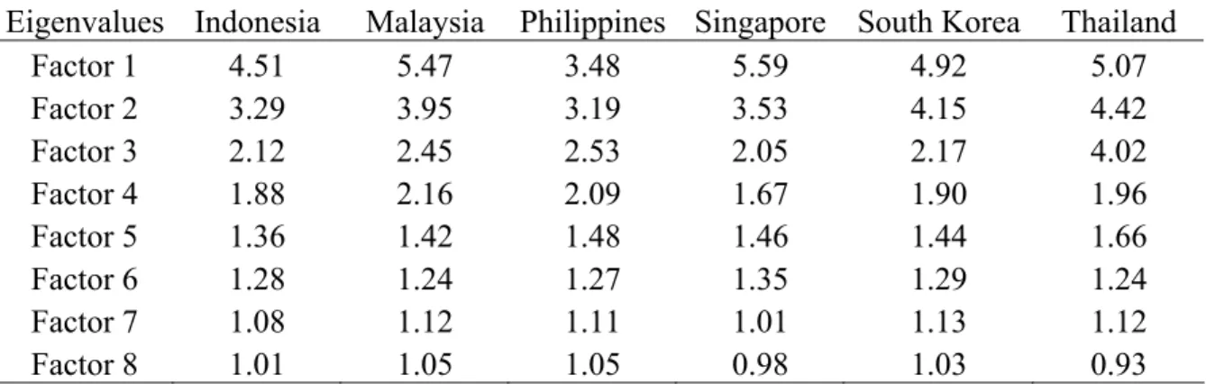
The following table shows the eigenvalues obtained. Notice that eight factors are retained for Singapore and Thailand even thought there are only seven eigenvalues above 1.0.
TABLE 1: Eigenvalues using a Principal Component Analysis
Eigenvalues Indonesia Malaysia Philippines Singapore South Korea Thailand
Factor 1 4.51 5.47 3.48 5.59 4.92 5.07 Factor 2 3.29 3.95 3.19 3.53 4.15 4.42 Factor 3 2.12 2.45 2.53 2.05 2.17 4.02 Factor 4 1.88 2.16 2.09 1.67 1.90 1.96 Factor 5 1.36 1.42 1.48 1.46 1.44 1.66 Factor 6 1.28 1.24 1.27 1.35 1.29 1.24 Factor 7 1.08 1.12 1.11 1.01 1.13 1.12 Factor 8 1.01 1.05 1.05 0.98 1.03 0.93
5.2.6 Step 5: Factor Score Estimation Method
The final step is to get factor scores. These scores in their whole represent a more parsimonious set of composite scores (i.e. composite variable scores for each Asian country of each factor). Different methods are available to compute the factor scores. This research utilizes the regression method.
Firstly, the original measured variables are changed into z scores with mean 0.0 and standard deviation of 1.0. These transformed variables present themselves under the matrix ZN × V. Then, the matrix of factor scores (FN × F) is obtained with the following
algorithm:
FN × F = ZN × V × R-1V × V × P(r)V × F,
where R-1
V × V is the inverse of the matrix of association and P(r)V × F is the rotated pattern
coefficient matrix.
The factor scores are computed with Huber-White robust standard errors.
These scores obtained serve as the independent variables in the multinomial logit model below. First differences in these factors are as well used as independent variables: They are the dynamics that Jacobs, Kuper and Lestano found to be statistically relevant in explaining probabilities of currency crises.
5.3 Part III : Multinomial Logit Analysis
The purpose of using a logit model is to compare the behaviour of economic variables (the indicators) during tranquil periods to their respective behaviours during pre-crisis episodes. In order to measure the probabilities of facing a crisis, a multinomial logit model is put in place so that it defines three possible outcomes. The model will be explained by presenting the different steps that allow its conception. Steps 1 and 2 construct variables used as tools to identify a crisis, whereas the following steps enter in the core of logit modeling.
5.3.1 Step 1 : Computing an Index
The first step when modeling an early warning system is to create an index that will serve to identify a crisis. The index used here is the one calculated by Bussière and
Fratzscher called the “exchange market pressure” index, EMPi,t (2002, p. 9), and is
computed as follows: For each country i and period t,
EMPi,t = ωREX [ RERi,t - RERi,t-1] + ωr (ri, t – ri, t-1) – ωres [resi,t – resi, t-1]
RERi,t-1 resi, t-1
EMPi,t is a weighted average of the change of the real effective exchange rate
(RER), the change in the interest rate (r) and the change in foreign exchange reserve (res). […] the weights ωRER, ωr and ωres are the relative precision of
each variable so as to give a larger weight to the variables with less volatility. The relative precision is defined as the inverse of the variance of each variable for all the countries over the full sample period (2002, p. 9).
Table A2 of the Appendix presents the sources of the three independent variables forming the pressure index, the transformation applied to EMPi,t and the explanation as to
why this index is used.
5.3.2 Step 2: Definition of a Crisis
The following step is to compute the occurrence of a currency crisis. Mathematically, Bussière and Fratzscher define the occurrence of a crisis in the following way: A currency crisis (CCi,t) happens
[…] at the event when the exchange market pressure (EMPi,t) variable is two
standard deviations (SD) or more above its country average EMPi (2002, p.
9):
CCi,t = 1 if EMPi,t > EMPi, + 2 SD(EMPi,)
0 if otherwise
5.3.3 Step 3: What the Model wants to Predict
This step is crucial in the sense that the researcher must decide whether his/her early warning model will attempt to predict the exact timing of a crisis or whether it will try to forecast the occurrence of the crisis within a specific time interval. So far in literature, the endeavour to master both the exact timing and the time horizon has not been taking care of, as it still represents an ambitious objective.
The paper of Bussière and Fratzscher aims to foresee crises occurring within a specific time horizon. This task is accomplished with the help of the currency crisis tool
(CCi,t). Indeed, a transformation of CCi,t is undertaken to create the variable Yi,t. This new
variable has three outcomes so that it addresses the post-crisis bias. The transformation is (2002, p. 21):
Yi,t = 1 if ∈ k = 1…12 [so that] CCit+k = 1
2 if ∈ k = 1…12 [so that] CCi
t-k = 1
0 if otherwise
where Y is the regime, i is the country and t is the time.
More precisely, “[…] a pre-crisis regime for the 12 months prior to the onset of a crisis (Yi,t = 1), a post/recovery regime for the crisis itself and 12 months following the
end of the crisis (Yi,t = 2), and a tranquil regime for all the other times (Yi,t = 0)” (2002, p.
21).
The choice of a 12-month window for the time to recover is made by a “strong empirical observation” (2002, p. 21) of the 32 countries in their simple. Additionally,
[…] our model attempts to predict whether a crisis will occur during a particular period of time, in this case in the coming 12 months. Choosing the length of this period requires striking balance between two opposite requirements. On the one hand, economic fundamentals tend to weaken closer an economy comes to a financial crisis, and therefore a crisis can be anticipated more reliably the closer the crisis is. But on the other hand, from a policy-maker’s perspective it is desirable to have as early an indication of economic weaknesses and vulnerabilities as possible in order to be able to take pre-emptive measures. […] the 12-month horizon provides what we believe is a good trade-off between these two issues (2002, p. 10).
One should finally notice that CCi,t is a contemporaneous variable whereas Yi,t is a
forward variable. From a practical point of view, the authors note that
Forwarding the left-hand side variable and using it on contemporaneous right-hand side variables allows a considerable simplification of the notation: otherwise we would need to include in the right-hand side all the 12 lags of the […] variables (2001, p. 21).
5.3.4 Interpretation of the Regimes
The tranquil regime (Yi,t = 0) is taken as the reference period (or base period) and
Prob (Yi,t = 0) = 1
1 + e(Xi,t-1β1) + e(Xi,t-1β2)
Prob (Yi,t = 1) = e(Xi,t-1β1)
1 + e(Xi,t-1β1) + e(Xi,t-1β2)
Prob (Yi,t = 2) = e(Xi,t-1β2)
1 + e(Xi,t-1β1) + e(Xi,t-1β2)
where X is the independent variable, i is the country and t is the time. These probability equations can be rearranged in the following way:
Prob (Yi,t = 1) = e(Xi,t-1β1)
Prob (Yi,t = 0)
And
Prob (Yi,t = 2) = e(Xi,t-1β2)
Prob (Yi,t = 0)
This indicates that
β1 measures the marginal effect of a change in the variable Xi,t-1 on the
probability of being in a pre-crisis period relative to the probability of being in the tranquil regime. Accordingly, β2 measures the marginal effect of a
change in the variable Xi,t-1 on the probability of being in a recovery period
relative to the probability of being in the tranquil regime (2002, p. 23).
The aim when constructing an early warning system model is to predict correctly if a market is vulnerable, thus more likely to fall into a crisis. With this definition in mind, the coefficient β1 therefore is the one to pay attention to. β2 will not be mentioned
further.
5.4 Results and Evaluation of the Performance of the Multinomial Logit Model using Factor Analysis
This section answers empirically the question raised earlier as to know if the Asian crisis of 1997 could have been more accurately predicted. In order to do so, a
measure of performance is computed, namely the signal-to-noise ratio. In fact, multiple ways of calculating this ratio exist, but with the purpose of comparing the model developed here to the models studied by Jacob, Kuper and Lestano, this present paper reproduces their calculations.
5.4.1 The Signal-to-Noise Ratio as a Measure of Performance
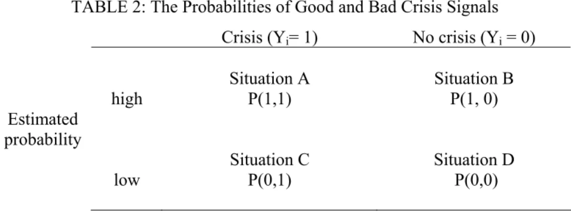
The signal-to-noise ratio is calculated from the four possibilities that an early warning system can produce:
1) The model might reveal a high estimated probability that a crisis is about to arise and a crisis indeed materializes: A correct call (a good signal) is then issued (P(1,1)).
2) The second possibility is when the model estimates the occurrence of a crisis (again with a high estimated probability) but no crisis in fact occurs (P(1,0)). The model consequently sends a wrong signal.
3) The model may estimate a low probability of an upcoming crisis but a crisis does occur (P(0,1)). In other words, the model missed it.
4) The model shows again a low estimated probability and no crisis takes place (P(0,0)). In that case, there is a correct called of a non-event.
All of these options are synthesized in the table below:
TABLE 2: The Probabilities of Good and Bad Crisis Signals Crisis (Yi= 1) No crisis (Yi = 0)
high Situation A P(1,1) Situation B P(1, 0) Estimated probability low Situation C P(0,1) Situation D P(0,0)
The goal of every early warning signal model is to predict as correctly as possible the situations A and D at the same time as minimising cases C and B. These later situations are in fact called noise and are also known as Type 1 and Type 2 errors,
respectively. One may notice that a missed call has much more ill-fated consequences than a wrong call.
The probabilities are calculated as follows:
P(1,1) = Σt ƥt* Уt Σt Уt P(1,0) = Σt ƥt * (1- Уt) Σt (1- Уt) P(0,1) = 1- P(1,1) P(0,0) = 1 - P(1,0)
where ƥt is the estimated probability from the multinomial logit model at time t and Уt is
the crisis index dummy equals to 1 in a pre-crisis regime 12 months before the start of a crisis, to 2 in a post/recovery regime for the crisis itself and 12 months following the end of the crisis and 0 otherwise (i.e. in a tranquil regime).
The signal-to-noise ratio is then calculated with the four possible probabilities: S = P(1,1) + P(0,0)
N P(1,0) + P(0,1)
5.4.2 The Results obtained by Jacobs, Kuper and Lestano (2004)
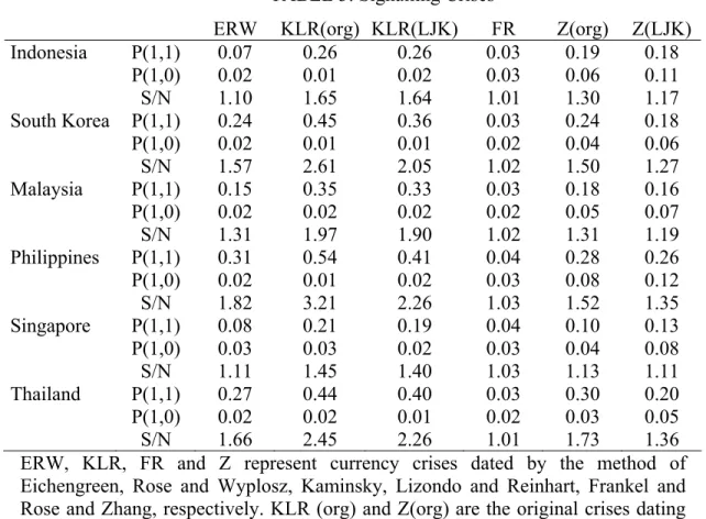
The following table lists the crisis signals, good and bad (P(1,1) and P(1, 0)) as well as the signal-to-noise ratio calculated by Jacobs, Kuper and Lestano for the six Asian countries, with monthly data from January 1977 until December 2001, using dynamic factor analysis with a two-outcome logit model. The analysis is performed on the researches developed by Eichengreen, Rose and Wyplosz (1995), Frankel and Rose (1996), Kaminsky, Lizondo and Reinhart (1998) and Zhang (2001) as well as versions of the mentioned papers of Kaminsky, Lizondo and Reinhart and Zhang modified by Jacobs, Kuper and Lestano.
TABLE 3: Signalling Crises
ERW KLR(org) KLR(LJK) FR Z(org) Z(LJK)
Indonesia P(1,1) 0.07 0.26 0.26 0.03 0.19 0.18 P(1,0) 0.02 0.01 0.02 0.03 0.06 0.11 S/N 1.10 1.65 1.64 1.01 1.30 1.17 South Korea P(1,1) 0.24 0.45 0.36 0.03 0.24 0.18 P(1,0) 0.02 0.01 0.01 0.02 0.04 0.06 S/N 1.57 2.61 2.05 1.02 1.50 1.27 Malaysia P(1,1) 0.15 0.35 0.33 0.03 0.18 0.16 P(1,0) 0.02 0.02 0.02 0.02 0.05 0.07 S/N 1.31 1.97 1.90 1.02 1.31 1.19 Philippines P(1,1) 0.31 0.54 0.41 0.04 0.28 0.26 P(1,0) 0.02 0.01 0.02 0.03 0.08 0.12 S/N 1.82 3.21 2.26 1.03 1.52 1.35 Singapore P(1,1) 0.08 0.21 0.19 0.04 0.10 0.13 P(1,0) 0.03 0.03 0.02 0.03 0.04 0.08 S/N 1.11 1.45 1.40 1.03 1.13 1.11 Thailand P(1,1) 0.27 0.44 0.40 0.03 0.30 0.20 P(1,0) 0.02 0.02 0.01 0.02 0.03 0.05 S/N 1.66 2.45 2.26 1.01 1.73 1.36 ERW, KLR, FR and Z represent currency crises dated by the method of Eichengreen, Rose and Wyplosz, Kaminsky, Lizondo and Reinhart, Frankel and Rose and Zhang, respectively. KLR (org) and Z(org) are the original crises dating schemes, KLR(LJK) and Z(LJK) are the versions of Lestano, Jacobs and Kuper. P(1,1)= the estimated probability is high and a crisis does occur; P(1,0)= the estimated probability is high and a crisis does not occur; S/N is the signal-to-noise ratio (2004, p. 21).
By differencing currency crisis dating schemes, Lestano, Jacobs and Kuper assess each of them as indicated by their respective power to signal a crisis. The authors conclude that the dating methodology presented by the original Kaminsky, Lizondo and Reinhart (1998) outperforms the other models with signal-to-noise ratios (S/N) higher than all the other signal-to-noise ratios calculated for each of the six countries.
The next step now is to calculate the signal-to-noise ratios of the model suggested in this present paper that differentiates itself by following not only the dating scheme of Bussière and Fratzscher, but also by applying their method of multinomial logit modeling.