Correcting the Errors: A Note on Volatility Forecast Evaluation Based on High-Frequency Data and Realized Volatilities

Texte intégral

(1)2002s-91. Correcting the Errors: A Note on Volatility Forecast Evaluation Based on High-Frequency Data and Realized Volatilities Torben G. Andersen, Tim Bollerslev, Nour Meddahi. Série Scientifique Scientific Series. Montréal Décembre 2002. © 2002 Torben G. Andersen, Tim Bollerslev, Nour Meddahi. Tous droits réservés. All rights reserved. Reproduction partielle permise avec citation du document source, incluant la notice ©. Short sections may be quoted without explicit permission, if full credit, including © notice, is given to the source..

(2) CIRANO Le CIRANO est un organisme sans but lucratif constitué en vertu de la Loi des compagnies du Québec. Le financement de son infrastructure et de ses activités de recherche provient des cotisations de ses organisationsmembres, d’une subvention d’infrastructure du ministère de la Recherche, de la Science et de la Technologie, de même que des subventions et mandats obtenus par ses équipes de recherche. CIRANO is a private non-profit organization incorporated under the Québec Companies Act. Its infrastructure and research activities are funded through fees paid by member organizations, an infrastructure grant from the Ministère de la Recherche, de la Science et de la Technologie, and grants and research mandates obtained by its research teams. Les organisations-partenaires / The Partner Organizations •École des Hautes Études Commerciales •École Polytechnique de Montréal •Université Concordia •Université de Montréal •Université du Québec à Montréal •Université Laval •Université McGill •Ministère des Finances du Québec •MRST •Alcan inc. •AXA Canada •Banque du Canada •Banque Laurentienne du Canada •Banque Nationale du Canada •Banque Royale du Canada •Bell Canada •Bombardier •Bourse de Montréal •Développement des ressources humaines Canada (DRHC) •Fédération des caisses Desjardins du Québec •Hydro-Québec •Industrie Canada •Pratt & Whitney Canada Inc. •Raymond Chabot Grant Thornton •Ville de Montréal. Les cahiers de la série scientifique (CS) visent à rendre accessibles des résultats de recherche effectuée au CIRANO afin de susciter échanges et commentaires. Ces cahiers sont écrits dans le style des publications scientifiques. Les idées et les opinions émises sont sous l’unique responsabilité des auteurs et ne représentent pas nécessairement les positions du CIRANO ou de ses partenaires. This paper presents research carried out at CIRANO and aims at encouraging discussion and comment. The observations and viewpoints expressed are the sole responsibility of the authors. They do not necessarily represent positions of CIRANO or its partners.. ISSN 1198-8177.

(3) Correcting the Errors: A Note on Volatility Forecast Evaluation Based on High-Frequency Data and Realized Volatilities* Torben G. Andersen†, Tim Bollerslev‡, Nour Meddahi§ Résumé / Abstract Cette note développe des méthodes d’ajustement, sans spécifier le modèle, qui corrigent le biais induit par les erreurs de mesures de la volatilité dans la mesure de performance des méthodes de prévision de la volatilité. Les procédures, qui utilisent la récente théorie asymptotique de Barndorff-Nielsen et Shephard (2002a), sont faciles à mettre en œuvre et très performantes dans les situations empiriques usuelles. En particulier, la prise en compte des erreurs de mesures dans les procédures de prévision de Andersen, Bollerslev, Diebold et Labys (2003), amène à des performances de prévision de la volatilité très élevées.. This note develops general model-free adjustment procedures for the calculation of unbiased volatility loss functions based on practically feasible realized volatility benchmarks. The procedures, which exploit the recent asymptotic distributional results in Barndorff-Nielsen and Shephard (2002a), are both easy-to-implement and highly accurate in empirically realistic situations. On properly accounting for the measurement errors in the volatility forecast evaluations reported in Andersen, Bollerslev, Diebold and Labys (2003), the adjustments result in markedly higher estimates for the true degree of return-volatility predictability.. Mots clés: Erreurs de mesure; méthode d’ajustement; volatilité intégrée, volatilité réalisée; données à haute fréquence; prévision de série chronologiques; régressions de Mincer-Zarnowitz. Keywords: Measurement errors; model-free adjustment procedures; integrated volatility; realized volatility; high-frequency data; time series forecasting; MincerZarnowitz regressions.. *. This work was supported by a grant from the National Science Foundation to the NBER (Andersen and Bollerslev), and from IFM2 and MITACS (Meddahi). Some of this material was circulated earlier as part of the paper "Analytical Evaluation of Volatility Forecasts." Detailed comments by Neil Shephard and discussions with Francis X. Diebold on closely related ideas have been very helpful. The third author thanks the Bendheim Center for Finance, Princeton University, for its hospitality during his visit and the revision of the paper. † Department of Finance, Kellogg School of Management, Northwestern University, Evanston, I1 60208, and NBER, USA, phone: 847-467-1285, e-mail: t-andersen@kellogg.northwestern.edu. ‡ Department of Economics, Duke University, Durham, NC 27708, and NBER, USA, phone: 919-660-1846, e-mail: boller@econ.duke.edu. § Département de sciences économiques, CIRANO, CIREQ, Université de Montréal, C.P. 6128, succursale Centreville, Montréal (Québec), H3C 3J7, Canada, phone: 514-343-2399, e-mail: nour.meddahi@umontreal.ca..

(4) 1. Introduction. The burgeoning literature on time-varying financial market volatility is abound with empirical studies in which competing models are evaluated and compared on the basis of their forecast performance. Contrary to the typical setting for economic forecast evaluation, the variable of interest in that context - the volatility - is not directly observable but rather inherently latent. Consequently, any ex-post assessment of forecast precision must contend with a fundamental errors-in-variable problem associated with the measurement of the realization of the forecasted variable. Growing recognition of the importance of this issue has led a number of recent studies to advocate the use of so-called realized volatilities, constructed from the summation of finely sampled squared high-frequency returns, as a practical method for improving the ex-post volatility measures. The recent paper by Andersen, Bollerslev, Diebold and Labys (2003) (henceforth ABDL) provides a leading example. The use of realized volatility as the practical benchmark may be justified by standard continuous-time arguments. Assuming that the sampling frequency of the squared returns utilized in the realized volatility computations approaches zero, the realized volatility consistently estimates the true (latent) integrated volatility. Importantly, the latter concept corresponds to the realization of the (cumulative) instantaneous variance process over the horizon of interest (see, e.g., ABDL, 2001; Barndorff-Nielsen and Shephard, 2001, 2002a,b; and Comte and Renault, 1998, for detailed discussions). Unfortunately, market microstructure frictions distort the measurement of returns at the highest frequencies so that, e.g., tick-by-tick return processes blatantly violate the theoretical semi-martingale restrictions implied by the no-arbitrage assumptions in continuous-time asset pricing models. These same features also bias empirical realized volatility measures constructed directly from the ultra high-frequency returns, so in practice the measures are instead typically constructed from intraday returns sampled at an intermediate frequency.1. As such, the integrated. volatility is invariably measured with error (see, e.g., the numerical calculations in Andreou and Ghysels, 2002, and Bai, Russell, and Tiao, 2000). The exact form of the measurement error will, of course, depend on the assumed model structure (see, e.g., Meddahi, 2002, for analytical calculations within the eigenfunction stochastic volatility class of models), but it will generally result in a downward bias in the estimated degree of predictability obtained 1 The daily realized volatilities in ABDL (2003) are based on the summation of squared half-hourly foreign exchange rate returns, but either 5-minute or 15-minute returns are other common choices in the literature.. 1.

(5) through any forecast evaluation criterion that simply uses the realized volatility in place of the true (latent) integrated volatility. Although this bias may be large (Andersen and Bollerslev, 1998), it is almost always ignored in empirical applications. This note addresses that issue by developing general model-free adjustment procedures that allow for the calculation of simple unbiased loss functions in realistic forecast situations. Moreover, the adjustments are simple to implement in practice. The derivation exploits the recent asymptotic (for increasing sampling frequency) distributional results in BarndorffNielsen and Shephard (2002a). Following Andersen and Bollerslev (1998) and ABDL (2003), we focus our forecast comparisons on the value of the coefficient of multiple correlation, or R2 , in the Mincer-Zarnowitz style regressions of the ex-post realized volatility on the corresponding model forecasts,2 but our procedures are general and could be applied in the adjustment of other loss functions used in the evaluation of any arbitrary set of volatility forecasts. On applying the procedures in the context of ABDL (2003), we obtain markedly higher estimates for the true degree of return-volatility predictability, with the adjusted R2 ’s exceeding their unadjusted counterparts by up to forty-percent. We proceed as follows. The first subsection below introduces the notions of integrated and realized volatility within the general class of continuous-time stochastic volatility models, along with the (feasible) asymptotic distribution theory due to Barndorff-Nielsen and Shephard (2002a). The development of the practical and easy-to-implement adjustment procedures is then presented in the next subsection, followed by our reassessment of the empirical evidence in ABDL (2003) related to the fit of the Mincer-Zarnowitz style volatility regressions. The Appendix presents the results from a small scale Monte Carlo simulation experiment that confirms the accuracy of the asymptotic approximations - which form the basis for our approach - for models calibrated to reflect empirically relevant and challenging specifications.. 2. Theory. We focus on a single asset traded in a liquid financial market. Assuming that the sample-path of the logarithmic price process, {pt , 0 ≤ t}, is continuous, the class of continuous-time stochastic volatility models employed in the finance literature is then conveniently expressed 2. This particular loss function is directly inspired by the work of Mincer and Zarnowitz (1969), and we will refer to the corresponding regressions as such; see also the discussion in Chong and Hendry (1986).. 2.

(6) in terms of the following generic stochastic differential equation (sde),. dpt = µt dt + σt dWt ,. (1). where Wt denotes a standard Brownian motion, and the drift term µt is (locally) predictable and of finite variation. To facilitate the discussion we will assume that the point-in-time, or spot, volatility process and the Brownian motion driving the price are (instantaneously) uncorrelated, or Corr(dσt , dWt ) = 0. However, the same (approximate) arguments carry over to the case of a non-zero correlation, as documented by, e.g., the simulation evidence in Barndorff-Nielsen and Shephard (2003), and the theoretical calculations for the class of eigenfunction stochastic volatility models in Meddahi (2002).. We further support. this contention for the measures utilized in the adjustments developed here by explicitly incorporating a realistic degree of leverage (negative contemporaneous return-volatility correlation) for one of the models analyzed within the Monte Carlo study reported on in the Appendix.. 2.1. Integrated and Realized Volatility. Although the sde in equation (1) is very convenient from a theoretical arbitrage-based pricing perspective, as emphasized by Andersen, Bollerslev and Diebold (2002), practical return calculations and volatility measurements are invariably restricted to discrete time intervals. In particular, focusing on the unit time interval, the one-period continuously compounded return for the price process in equation (1) is formally given by,3 Z. t. Z. rt ≡ pt − pt−1 =. t. µu du + t−1. σu dWu .. (2). t−1. Hence, conditional on the sample-path realizations of the drift and instantaneous volatility processes, {µu , t−1 ≤ u ≤ t} and {σu , t−1 ≤ u ≤ t}, respectively, the one-period returns are Gaussian with conditional mean equal to the first integral on the right-hand-side of equation (2), and conditional variance equal to the integrated volatility, Z. t. IVt ≡. σu2 du.. (3). t−1 3. For notational simplicity, we focus our discussion on one-period return and volatility measures, but the general results and associated measurement error adjustment extend in a straightforward manner to the multi-period case.. 3.

(7) The integrated volatility therefore affords a natural measure of the (ex-post) return variability.4 Of course, integrated volatility is not directly observable. However, by the theory of quadratic variation, the corresponding realized volatility defined by the summation of the (h). 1/h intra-period squared returns, rt. ≡ pt − pt−h ,. RVt (h) ≡. 1/h X. (h)2. rt−1+ih ,. (4). i=1. where 1/h is assumed to be an integer, converges uniformly in probability to IVt as h → 0. Moreover, under additional mild regularity conditions on the process in (1), BarndorffNielsen and Shephard (2002a) have recently established that for h → 0, and conditional on {σu , t − 1 ≤ u ≤ t}, the realized volatility error is approximately distributed as, RVt (h) − IVt ∼ h1/2 IQt (h)1/2 zt ,. (5). where zt is N (0, 1), and the integrated quarticity, Z. t. σu4 du ,. IQt ≡ 2. (6). t−1. is consistently estimated by the (standardized) realized quarticity 1/h. 1 2 X (h)4 r . RQt (h) ≡ h 3 i=1 t−1+ih. (7). This remarkable set of asymptotic results allow for general model-free approximations to the distribution of the realized volatility error. Importantly, from the present perspective, equation (5) implies that the time t+1 realized volatility error is (approximately) serially uncorrelated and orthogonal to any variables (volatility forecasts) in the time t information set. This justifies the common use of realized volatility as a convenient simple and unbiased, albeit potentially noisy, benchmark in ex-post volatility forecast evaluations. Building on these general results, we next develop a set of easy-to-implement procedures that may be used to properly account for the corresponding measurement errors in practical forecast situations. 4. The integrated volatility also plays a crucial role in the pricing of options; see, e.g., Garcia, Ghysels, and Renault (2002).. 4.

(8) 2.2. Practical Measurement Error Adjustments. The consistency and asymptotic normality results discussed in the previous section rely on the (conceptual) idea of an ever increasing number of finer sampled high-frequency returns, or h → 0. However, as previously noted, the requisite semi-martingale property of returns invariably breaks down at ultra-high frequencies, so that in actual applications market microstructure frictions in effect put a limit on the number of return observations per unit time interval ∆ that may be used productively in the computation of the realized volatility measures; i.e., h ≥ 1/∆ > 0. As such, the realized volatility will necessarily be subject to a finite-sample (non-zero h) measurement error vis-a-vis the true (latent) integrated volatility. Assuming that the underlying continuous time process satisfies a weak uniform integrability condition so that the consistency of RQt (h) for IQt also guarantees convergence in mean (see, e.g., Billingsley, 1994, and Hoffmann-Jørgensen, 1994), it follows directly from equation (5) that for small values of h,. V ar[IVt ] ≈ V ar[RVt (h)] − hE[RQt (h)].. (8). Thus, any MSE type forecast evaluation criteria based on a comparison of the volatility forecasts with the ex-post RVt (h) in place of IVt (h) will on average over-estimate the true variability of the forecast errors by hE[RQt (h)]. In particular, consider the MincerZarnowitz regression of the ex-post realized volatility on a set of predetermined regressors (volatility forecasts) commonly used as guide in evaluating and comparing the performance of competing volatility models.. It follows that the (feasible) R2 from this regression. will under-estimate the true predictability as measured by the (infeasible) R2 from the regression of the future (latent) integrated volatility on the same set of predetermined regressors (volatility forecasts) by the multiplicative factor:. V ar[RVt (h)]/V ar[IVt ] ≈. V ar[RVt (h)]/{V ar[RVt (h)] − hE[RQt (h)]}.5 Meanwhile, the predictive regressions and related loss functions reported in the extant volatility literature are often formulated in terms of the realized standard deviation, RVt (h)1/2 , or the logarithmic standard deviation, log RVt (h)1/2 . To properly gauge the true predictability in those situations the sample variances of the transformed realized volatilities 5. As previously noticed by Meddahi (2002), the approximation in (8) also allows for the construction of more efficient (in the sense of MSE) model-free integrated volatility estimates, by downweighting the realized volatility by the multiplicative factor {V ar[RVt (h)] − hE[RQt (h)]}/V ar[RVt (h)] and adding the constant {E[RVt (h)]hE[RQt (h)]}/V ar[RVt (h)].. 5.

(9) 1/2. may be similarly replaced by (feasible) expressions for the true (latent) variances, V ar[IVt 1/2. and V ar[log IVt. ]. ], respectively.6 To this end, it follows from equation (5) and a second-order. Taylor series expansion of the square-root function of RVt (h) around IVt that, conditional on the sample-path realization of the (latent) point-in-time volatility process, 1/2. RVt (h)1/2 ≈ IVt. +. 1 1/2 −1/2 1/2 1 −3/2 h IVt IQt zt − hIVt IQt zt2 , 2 8. for small values of h. Subject to the necessary uniform integrability conditions on the underlying continuous-time process ensuring convergence in mean of the relevant quantities, it therefore follows that 1/2. V ar[IVt. ] ≈ E[RVt (h)] − {E[RVt (h)1/2 ] +. h E[RVt (h)−3/2 RQt (h)]}2 . 8. (9). The variance of the square-root of the realized volatility, as used in a number of previous empirical studies, obviously exceeds the expression in (9) by the absence of the second (positive) term in the last squared bracket. This in turn will result in a downward bias in the R2 ’s from the (feasible) predictive regressions formulated in terms of RVt (h)1/2 in place 1/2. of IVt. .. By similar arguments, 1/2. log RVt (h) ≈ log IVt + h1/2 IVt−1 IQt zt −. 1 hIVt−2 IQt zt2 , 2. and, 1/2. [log RVt (h)]2 ≈ [log IVt ]2 + 2h1/2 IVt−1 [log IVt ]IQt zt + hIVt−2 (1 − log IVt )IQt zt2 . Thus, subject to the necessary integrability conditions, it follows that, V ar[log IVt ] ≈ E[[log RVt (h)]2 ] − hE[RVt (h)−2 (1 − log RVt (h))RQt (h)] 1 − {E[log RVt (h)] + hE[RVt (h)−2 RQt (h)]}2 . 2. (10). The transformation of the asymptotic distribution in equation (5) to a logarithmic scale discussed in Barndorff-Nielsen and Shephard (2002b, 2003) provides an alternative approximation to the distribution of the logarithmic realized volatility. 1/2. 6. Any transformed unbiased forecast for IVt+1 will generally not be unbiased for IVt+1 or log IVt+1 . However, allowing for a non-zero intercept and a slope coefficient different from unity in the Mincer-Zarnowitz regression of the future transformed realized volatility on the transformed forecast explicitly corrects this bias; see also the discussion in Andersen, Bollerslev and Meddahi (2002).. 6.

(10) The accuracy of the distributional assumption and second-order Taylor series expansions underlying the (feasible) expressions for the latent variances in equations (8)-(10) are underscored by the simulation results reported in the Appendix. Similar arguments could, of course, be applied for any other twice continuously differentiable function of integrated volatility in order to obtain an approximate value for V ar[f (IVt )], in turn allowing for simple model-free approximations to the true (infeasible) R2 ’s that would obtain in the hypothetical regressions of f (IVt ) on any forecasts by scaling the (feasible) R2 ’s from the corresponding regressions based on f (RVt (h)) by the multiplicative adjustment factor, V ar[f (RVt (h))]/{V ar[f (IVt (h))]}. We next apply these ideas in re-interpreting the empirical evidence related to the Mincer-Zarnowitz volatility regressions reported in ABDL (2003).. 2.3. ABDL (2003) Revisited. The forecast comparisons in ABDL (2003) are based on daily realized volatilities constructed from high-frequency half-hourly, or h=1/48, spot exchange rates for the U.S. dollar, the Deutschemark and the Japanese yen spanning twelve-and-a-half years.7 Separate forecast evaluation regressions are reported for the “in-sample” period comprised of the 2,449 “regular” trading days from December 1, 1986 through December 1, 1996, and the shorter “out-of-sample” forecast period consisting of the 596 days from December 2, 1996 through June 30, 1999. Separate results are also reported for one-day-ahead and ten-days-ahead forecasts. Interestingly, for all series and both sample periods and forecast horizons, a simple AR(5) model estimated directly from the realized volatilities generally performs as well or better than any of the many alternative models considered, including several GARCH type models estimated directly to the high-frequency data (both with and without corrections for the pronounced intradaily seasonal pattern in volatility). The representative R2 ’s for the DM/$, Yen/$, and Yen/DM forecast regressions for RVt+1 (1/48), RVt+1 (1/48)1/2 , log RVt+1 (1/48)1/2 , RVt+10,10 (1/48), RVt+10,10 (1/48)1/2 , and log RVt+10,10 (1/48)1/2 , where RVt+10,10 (1/48) ≡ RVt+1 (1/48) + RVt+2 (1/48) + ... + RVt+10 (1/48), as reported in ABDL (2003) and the accompanying appendix, are given in square brackets in Table 1.8 7. The high-frequency data were generously provided by Olsen & Associates in Z¨ urich, Switzerland; see Dacorogna, Gencay, M¨ uller, Olsen and Pictet (2001) for further discussion of the data capture, filtering, and return construction. 8 The out-of-sample period contains a “once-in-a-generation” move in the Japanese Yen on October 8, 1998. Somewhat higher R2 ’s, but qualitatively similar results, were obtained by excluding this and the neighboring two days; see ABDL (2003) and the accompanying appendix for further discussion and sensitivity analysis along these lines.. 7.

(11) By failing to account for the measurement errors in the future realized volatilities, these R2 ’s understate the true degree of predictability in the (latent) integrated volatilities. This problem is rectified by the main entries in Table 1, which report the adjusted R2 ’s obtained by applying the (feasible) asymptotic approximations in equations (8)-(10) along with the relevant multiplicative adjustment factors.9 The results are quite striking. For some of the forecasts horizons and rates, the “true” R2 ’s exceed the standard predictive R2 ’s, as reported in ABDL (2003), by up to forty percent. For instance, the in-sample, one-day-ahead R2 for the DM/$ series given in the very first entry in the table equals 0.219, whereas the true (albeit estimated) R2 is substantially higher at 0.314. As such, the results highlight the importance of appropriately adjusting for measurement error when assessing the quality of volatility forecasts in practical empirical applications. Interestingly, the numerical values for the adjusted R2 ’s for the DM-dollar series in Table 1 are quite close to the exact theoretical R2 ’s implied by the specific two-factor affine diffusion discussed in Andersen, Bollerslev and Meddahi (2002). This is especially noteworthy because the parameter values for this model are based on the identical DM-dollar sample underlying the results reported on in Table 1. This suggests that the simple AR(5) models for the realized volatilities estimated in ABDL (2003) - when adjusted for the measurement error problem - capture a degree of predictability that is consistent with that implied by a conventional two-factor affine model. This type of benchmarking of the true predictive power of such reduced-form forecast procedures relative to that of a specific continuous-time volatility model would, of course, be impossible without the type of measurement error correction developed here.. 9. The adjustments are constructed separately for each series and for the in-sample and out-of-sample periods using the corresponding realized volatility and quarticity series.. 8.

(12) Table 1 ABDL (2003) Adjusted Predictive R2 ’s. In-Sample, One-Day-Ahead DM/$ Yen/$ Yen/DM Out-of-Sample, One-Day-Ahead DM/$ Yen/$ Yen/DM In-Sample, Ten-Days-Ahead DM/$ Yen/$ Yen/DM Out-of-Sample, Ten-Days-Ahead DM/$ Yen/$ Yen/DM. 3. IV. IV 1/2. log IV 1/2. 0.314 [0.219] 0.315 [0.229] 0.450 [0.361]. 0.399 [0.351] 0.482 [0.431] 0.412 [0.374] 0.476 [0.433] 0.559 [0.499] 0.630 [0.567]. 0.200 [0.158] 0.230 [0.197] 0.215 [0.189]. 0.296 [0.246] 0.350 [0.285] 0.366 [0.338] 0.419 [0.373] 0.378 [0.344] 0.483 [0.424]. 0.411 [0.374] 0.386 [0.355] 0.536 [0.513]. 0.463 [0.436] 0.499 [0.473] 0.414 [0.396] 0.424 [0.407] 0.606 [0.589] 0.653 [0.637]. 0.182 [0.168] 0.197 [0.187] 0.186 [0.178]. 0.209 [0.195] 0.228 [0.213] 0.287 [0.279] 0.347 [0.336] 0.301 [0.293] 0.401 [0.390]. Concluding Remarks. Building on the recent theoretical results of Barndorff-Nielsen and Shephard (2002a), this note develops a set of simple and practically feasible expressions for calculating true measures of return volatility predictability relative to that of the corresponding underlying (latent) integrated volatility. The procedures are general and could be applied in the evaluation of any volatility forecasts. On specifically applying the procedures to the ex-post forecast evaluation regressions reported in ABDL (2003), we document sizeable downward biases in terms of the previously reported predictive powers. More generally, the practical techniques developed here hold the promise for further development of new and improved easy-toimplement volatility forecasting procedures guided by proper benchmark comparisons. The techniques should also prove useful in more effectively calibrating the type of continuous-time models routinely employed in modern asset pricing theories.. 9.

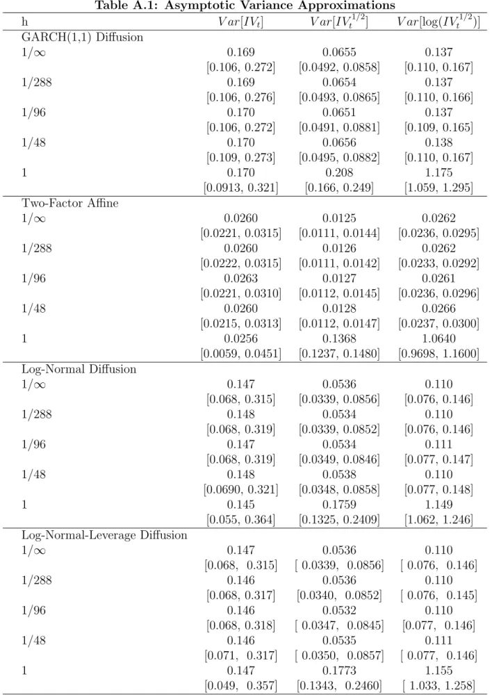
(13) Appendix: Finite Sample Variance Approximations To assess the accuracy of the distributional assumptions and second-order Taylor series expansions underlying the asymptotic approximations for the variances of the latent integrated volatilities in empirically relevant specifications and sample sizes compatible with those of ABDL (2003), Table A.1 reports the simulated medians and ninety-percent confidence intervals (in square brackets) across 100 replications, each consisting of 2,500 “days.” The table reports the results for four different continuous-time models along with 1/h = 288, 96, 48, and 1, corresponding to the use of “5-minute,” “15-minute,” “half-hourly,” and “daily” returns. In the first three models we assume the mean to be zero, or dpt = σt dWt . The numbers in the first panel refer to the GARCH(1,1) diffusion analyzed in Andersen and Bollerslev (1998), dσt2 = 0.035(0.636 − σt2 )dt + 0.144dBt , where the Bt denotes a standard Brownian motion. The second panel gives the results for the two-factor 2 2 2 affine diffusion estimated by Bollerslev and Zhou (2002), where σt2 = σ1,t + σ2,t , dσ1,t = 2 2 2 0.571(0.326−σ1,t )dt+0.229σ1,t dB1,t , dσ2,t = 0.076(0.179−σ2,t )dt+0.110σ2,t dB2,t , and the two Brownian motions are assumed to be independent. These parameter values were obtained from estimation based on the identical DM-dollar sample used in ABDL (2003). The two final sets of numbers refer to the log-normal diffusion reported in Andersen, Benzoni and Lund (2002) with volatility dynamics governed by d log(σt2 ) = −0.014[0.838+log(σt2 )]dt+0.115dBt . The results in the third panel imposes a zero mean return. The final panel is based on the identical volatility specification, but the log-price dynamics are now given by √ dpt = 0.031dt + σt [ 1 − 0.5762 dBt − 0.576dWt ]. This representation therefore includes a positive mean return and, more importantly, a strong leverage effect through the negative contemporaneous correlation between the return and volatility innovations. It is evident that the simulated medians and ninety-percent confidence intervals for 1/2 1/2 the asymptotic approximations to V ar[IVt ], V ar[IVt ] and V ar[log(IVt )] are extremely close to the simulated sampling distributions for the true variances (labelled h = 1/∞) as long as the frequency of the returns used in the calculation of the realized volatility and quarticity measures, RVt (h) and RQt (h), respectively, exceeds half-an-hour, or h ≤ 1/48. These results are directly in line with the earlier simulation evidence related to the accuracy of the underlying asymptotic approximation in equation (5) for other models reported in Barndorff-Nielsen and Shephard (2002a,b, 2003) and Meddahi (2002). Most noteworthy are the near identical results for the log-volatility diffusion model with and without the leverage effect. The asymptotic approximations are clearly robust to this - for equity returns important - feature of the data generating process.. 10.

(14) Table A.1: Asymptotic Variance Approximations 1/2 1/2 h V ar[IVt ] V ar[IVt ] V ar[log(IVt )] GARCH(1,1) Diffusion 1/∞ 0.169 0.0655 0.137 [0.106, 0.272] [0.0492, 0.0858] [0.110, 0.167] 1/288 0.169 0.0654 0.137 [0.106, 0.276] [0.0493, 0.0865] [0.110, 0.166] 1/96 0.170 0.0651 0.137 [0.106, 0.272] [0.0491, 0.0881] [0.109, 0.165] 1/48 0.170 0.0656 0.138 [0.109, 0.273] [0.0495, 0.0882] [0.110, 0.167] 1 0.170 0.208 1.175 [0.0913, 0.321] [0.166, 0.249] [1.059, 1.295] Two-Factor Affine 1/∞ 0.0260 0.0125 0.0262 [0.0221, 0.0315] [0.0111, 0.0144] [0.0236, 0.0295] 1/288 0.0260 0.0126 0.0262 [0.0222, 0.0315] [0.0111, 0.0142] [0.0233, 0.0292] 1/96 0.0263 0.0127 0.0261 [0.0221, 0.0310] [0.0112, 0.0145] [0.0236, 0.0296] 1/48 0.0260 0.0128 0.0266 [0.0215, 0.0313] [0.0112, 0.0147] [0.0237, 0.0300] 1 0.0256 0.1368 1.0640 [0.0059, 0.0451] [0.1237, 0.1480] [0.9698, 1.1600] Log-Normal Diffusion 1/∞ 0.147 0.0536 0.110 [0.068, 0.315] [0.0339, 0.0856] [0.076, 0.146] 1/288 0.148 0.0534 0.110 [0.068, 0.319] [0.0339, 0.0852] [0.076, 0.146] 1/96 0.147 0.0534 0.111 [0.068, 0.319] [0.0349, 0.0846] [0.077, 0.147] 1/48 0.148 0.0538 0.110 [0.0690, 0.321] [0.0348, 0.0858] [0.077, 0.148] 1 0.145 0.1759 1.149 [0.055, 0.364] [0.1325, 0.2409] [1.062, 1.246] Log-Normal-Leverage Diffusion 1/∞ 0.147 0.0536 0.110 [0.068, 0.315] [ 0.0339, 0.0856] [ 0.076, 0.146] 1/288 0.146 0.0536 0.110 [0.068, 0.317] [0.0340, 0.0852] [ 0.076, 0.145] 1/96 0.146 0.0532 0.110 [0.068, 0.318] [ 0.0347, 0.0845] [0.077, 0.146] 1/48 0.146 0.0535 0.111 [0.071, 0.317] [ 0.0350, 0.0857] [ 0.077, 0.146] 1 0.147 0.1773 1.155 [0.049, 0.357] [0.1343, 0.2460] [ 1.033, 1.258] 11.

(15) References Andersen, T.G., L. Benzoni and J. Lund (2002), “An Empirical Investigation of ContinuousTime Equity Return Models,” Journal of Finance, 57, 1239-1284. Andersen, T.G. and T. Bollerslev (1998), “Answering the Skeptics: Yes, Standard Volatility Models Do Provide Accurate Forecasts,” International Economic Review, 39, 885-905. Andersen, T.G., T. Bollerslev and F.X. Diebold (2002), “Parametric and Nonparametric Volatility Measurement,” in Y. A¨ıt-Sahalia and L.P. Hansen (Eds.), Handbook of Financial Econometrics, forthcoming. Andersen, T.G., T. Bollerslev, F.X. Diebold and P. Labys (2001), “The Distribution of Exchange Rate Volatility,” Journal of the American Statistical Association, 96, 42-55. Andersen, T.G., T. Bollerslev, F.X. Diebold and P. Labys (2003), “Modeling and Forecasting Realized Volatility,” Econometrica, forthcoming. Andersen, T.G., T. Bollerslev, and N. Meddahi (2002), “Analytic Evaluation of Volatility Forecasts,” unpublished manuscript, Northwestern, Duke, and University of Montreal. Andreou, E. and E. Ghysels (2002), “Rolling-Sampling Volatility Estimators: Some New Theoretical, Simulation and Empirical Results,” Journal of Business and Economic Statistics, 20, 363-276. Bai, X., J.R. Russell, and G.C. Tiao (2000), “Beyond Merton’s Utopia: Effects of NonNormality and Dependence on the Precision of Variance Estimates using High-frequency Financial Data,” unpublished manuscript, University of Chicago. Barndorff-Nielsen, O.E. and N. Shephard (2001), “Non-Gaussian Ornstein-Uhlenbeck-based Models and Some of Their Uses in Financial Economics,” Journal of the Royal Statistical Society, B, 63, 167-207. Barndorff-Nielsen, O.E. and N. Shephard (2002a), “Econometric Analysis of Realised Volatility and its Use in Estimating Stochastic Volatility Models,” Journal of the Royal Statistical Society, B, 64, 253-280. Barndorff-Nielsen, O.E. and N. Shephard (2002b), “Estimating Quadratic Variation Using Realised Variance,” Journal of Applied Econometrics, 17, 457-477. Barndorff-Nielsen, O.E. and N. Shephard (2003), “How Accurate is the Asymptotic Approximation to the Distribution of Realised Volatility?,” in Identification and Inference for Econometric Models: A Festschrift for Thomas J. Rothenberg, D. Andrews, J. Powell, P. Ruud, and J. Stock eds., Cambridge University Press, forthcoming. Billingsley, P. (1994), Probability and Measure, Third Edition, New-York: John Wiley & Sons. Bollerslev, T. and H. Zhou (2002), “Estimating Stochastic Volatility Diffusion Using Conditional Moments of Integrated Volatility,” Journal of Econometrics, 109, 33-65. Chong, Y.Y. and D. Hendry (1986), “Econometric Evaluation of Linear Macro-Economic Models,” Review of Economic Studies, 53, 671-690. Comte, F. and E. Renault (1998), “Long Memory in Continuous Time Stochastic Volatility Models,” Mathematical Finance, 8, 291-323. Dacorogna, M.M., R. Gencay, U.A. M¨ uller, R.B. Olsen, and O.V. Pictet (2001), An Introduction to High-Frequency Finance, San Diego: Academic Press. Garcia, R., E. Ghysels and E. Renault (2002), “Option Pricing Models,” in Y. A¨ıt-Sahalia and L.P. Hansen (Eds.), Handbook of Financial Econometrics, forthcoming. Hoffman-Jørgensen, J. (1994), Probability with a View Toward Statistics, Volume 1, Chapman and Hall Probability Series, New-York: Chapman & Hall. Meddahi, N. (2001), “An Eigenfunction Approach for Volatility Modeling,” CIRANO working paper, 2001s-70. Meddahi, N. (2002), “A Theoretical Comparison Between Integrated and Realized Volatility,” Journal of Applied Econometrics, 17, 479-508. Mincer, J. and V. Zarnowitz (1969), “The Evaluation of Economic Forecasts,” in J. Mincer (Ed.), Economic Forecasts and Expectation, National Bureau of Research, New York.. 12.

(16)