Ardia: Corresponding author. Département de finance, assurance et immobilier, Université Laval, Québec (Québec), Canada
david.ardia@fsa.ulaval.ca
Hoogerheide: Department of Econometrics, Vrije Universiteit Amsterdam, The Netherlands
l.f.hoogerheide@vu.nl
We are grateful to Kris Boudt, Michel Dubois, Attilio Meucci, Istvan Nagi, Stefano Puddu and Enrico Schumann for useful comments. Any remaining errors or shortcomings are the authors’ responsibility.
Cahier de recherche/Working Paper 13-13
Cross-Sectional Distribution of GARCH Coefficients across S&P 500
Constituents : Time-Variation over the Period 2000-2012
David Ardia
Lennart F. Hoogerheide
Abstract:
We investigate the time-variation of the cross-sectional distribution of asymmetric
GARCH model parameters over the S&P 500 constituents for the period 2000-2012. We
find the following results. First, the unconditional variances in the GARCH model
obviously show major time-variation, with a high level after the dot-com bubble and the
highest peak in the latest financial crisis. Second, in these more volatile periods it is
especially the persistence of deviations of volatility from is unconditional mean that
increases. Particularly in the latest financial crisis, the estimated models tend to
Integrated GARCH models, which can cope with an abrupt regime-shift from low to high
volatility levels. Third, the leverage effect tends to be somewhat higher in periods with
higher volatility. Our findings are mostly robust across sectors, except for the technology
sector, which exhibits a substantially higher volatility after the dot-com bubble. Further,
the financial sector shows the highest volatility during the latest financial crisis. Finally, in
an analysis of different market capitalizations, we find that small cap stocks have a
higher volatility than large cap stocks where the discrepancy between small and large
cap stocks increased during the latest financial crisis. Small cap stocks also have a
larger conditional kurtosis and a higher leverage effect than mid cap and large cap
stocks.
Keywords: GARCH, GJR, equity, leverage effect, S&P 500 universe
Electronic copy available at: http://ssrn.com/abstract=2226406
1. Introduction
Investigation of volatility dynamics has attracted many academics and practitioners, as this is of substan-tial importance for risk management and derivatives pricing. Since the seminal paper byBollerslev(1986),
GARCH-type models have been widely used in financial econometrics for the forecasting of volatility.
These are nowadays standard models in risk management: they are easy to understand and interpret and available in many statistical packages.
Volatility tends to rise more in response to bad news than to good news and this phenomenon is espe-cially true on equity markets. This effect was observed byBlack(1976) and is referred to as the leverage
effectin the financial literature. One explanation of this empirical fact is that negative returns increase fi-nancial leverage which extends the company’s risk and therefore the variance. To cope with this stylized
fact, we use the GJR model of Glosten et al. (1993). In this setting, the conditional variance can react asymmetrically depending on the sign of the past shocks due to the introduction of dummy variables.
This note investigates the cross-sectional distribution of GJR-Student-t model parameters over con-stituents of the the S&P 500 index. Our aim is to investigate the time-variation of the estimated parameters
for a large universe of equities in the period 2000-2012. We first consider the whole universe of S&P 500 equities and then compare the results for different industries and sizes.
2. Model specification
As in McNeil and Frey (2000), the model starts with an AR(1) component in order to filter a possi-ble autoregressive part of the equity log-returns. For the volatility dynamics, we rely on the asymmetric
GJR(1,1) specification byGlosten et al.(1993).
More specifically, in the AR(1)-GJR(1,1)-Student-t model the log-returns rtare expressed as:
rt= µ + ρ rt−1+ ut (t = 1, . . . , T )
ut= σtεt εt∼ iid S(0, 1, ν)
σt2= ω + (α + γ 1{ut−1≤ 0}) u2t−1+ β σt−12 ,
(1)
where we require ω > 0 and α, γ, β ≥ 0 to ensure a positive conditional variance. 1{} denotes the
indicator function, whose value is one if the constraint holds and zero otherwise. Covariance stationarity
constraints have been imposed in the estimation, ie, α + γ/2 + β < 1, ensuring the existence of the
unconditional variance given by ω/(1−α−γ/2−β). For the distribution of the innovations εt, we consider
the standardized Student-t distribution (with variance one, where we impose the restriction ν > 2). The
Student-t distribution is probably the most commonly used alternative to the Gaussian for modeling stock returns and allows modeling fatter tails than the Gaussian. The model is fitted by maximum likelihood. We
rely on the rolling-window approach where 500 log-returns – ie, approximately two trading years – are used to estimate the model. The reason for using a relatively short and moving window of data is that we are
interested in the possible time-variation of the parameters.
3. Results and discussion
We estimate the model on all constituents of the S&P 500 index (using the constituents as of June 2012)
for a period ranging from January 1, 2000, to June 26, 2012, thus representing more than eleven years of daily data. The data are then filtered for liquidity followingLesmond et al.(1999). In particular, we remove
the time series with less than 1500 data points history, with more than 10% of zero returns and more than two trading weeks of constant price. This filtering approach reduces the database to 406 equities for which
the adjusted daily closing prices, the industry codes and the market capitalization are downloaded from Datastream.
3.1. Overall results
We report first the cross-sectional distribution of the estimated unconditional variance ˆω/(1 − ˆα − ˆγ/2 − ˆ
β) over time. The left-hand side of Figure1 displays the median (blue), 50% area (green) and 95% area
(red) of the unconditional variance for the 406 GJR models fitted over time. We can notice a clearly higher
unconditional volatility after the dot-com bubble and in the latest financial crisis, periods when the S&P 500 index had troughs; see the left-hand side of Figure2.
The right-hand side of Figure1displays the cross-sectional distribution of the estimated persistence ˆα + ˆ
γ/2 + ˆβ over time. In more volatile periods the persistence of deviations of volatility from its unconditional
mean increases substantially.
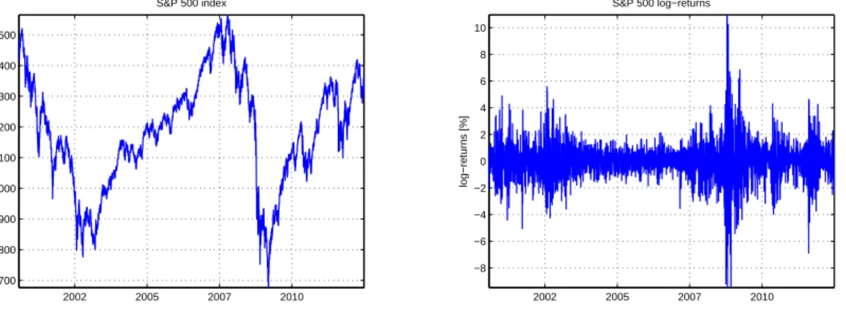
Figure 1: Left: Cross-sectional distribution plot of the unconditional volatility for the 406 GJR models fitted over time on the S&P 500 universe constituents. Right: Cross-sectional distribution plot of the persistence. Median (blue), 50% area (green), 95% area (red) 2002 2005 2007 2010 700 800 900 1000 1100 1200 1300 1400 1500 S&P 500 index 2002 2005 2007 2010 −8 −6 −4 −2 0 2 4 6 8 10 S&P 500 log−returns log−returns [%]
Figure 2: Left: S&P 500 level for our data window of years 2000–2012. Right: S&P 500 log-returns.
Particularly in the latest financial crisis, the estimated models tend to Integrated GARCH models (with ˆ
α + ˆγ/2 + ˆβ tending to 1), which can cope with a regime-shift from low to high volatility levels. That is, in
these estimated GJR models the volatility shows very little mean-reversion.
We notice that in the latest financial crisis, the set of persistence parameters of different stocks seems tighter to one than it has ever been before, which can reflect an abrupt regime-shift in volatility for (almost)
all stocks. In the previous trough after the Internet bubble, the changes of the volatility were more gradual (at least for a considerable subset of the stocks), where for many stocks there was clear evidence for substantial
mean-reversion of the volatility within each estimation window of 500 days. See also the right-hand side of Figure2that shows that the behavior of the log-returns on the S&P 500 index changed more abruptly in the
latest financial crisis.
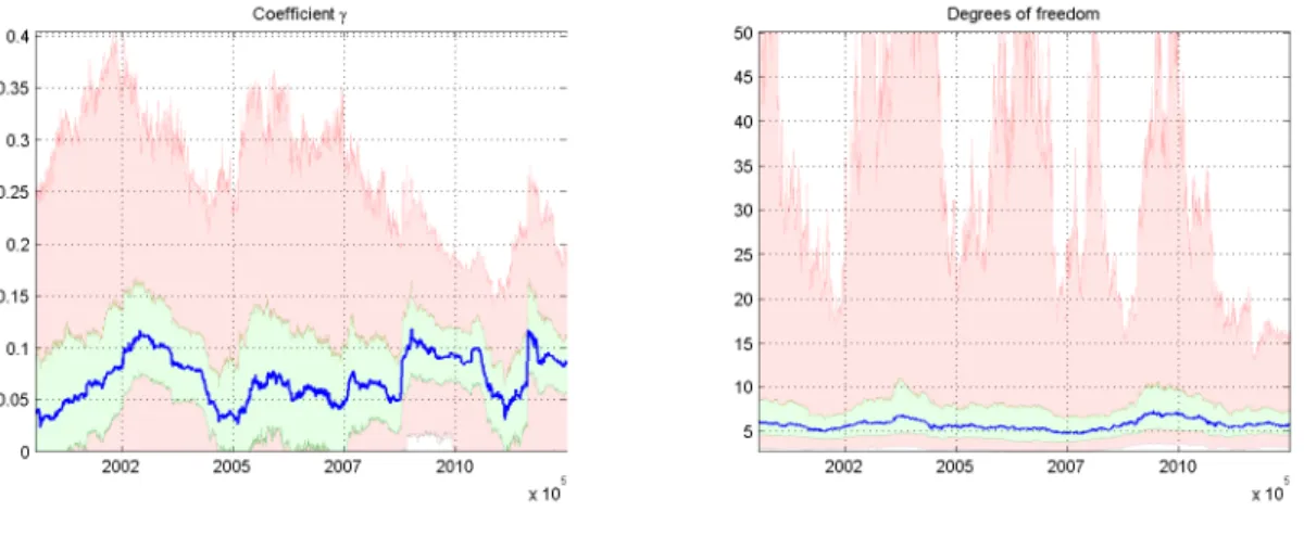
The left-hand side of Figure3displays the cross-sectional distribution of the estimated leverage
coef-ficient ˆγ over time, which follows a peculiar pattern. In the latest financial crisis, the leverage coefficients across S&P 500 stocks were not higher than in the trough after the dot-com bubble. However, the lower
bound of the 95% interval shows that the latest financial crisis is the first time (in the period 2000-2012) when more than 97.5% of the stocks had a strictly positive estimated leverage coefficient. This stresses how
widely the credit crunch affected the response of markets to bad news.
Figure 3: Left: Cross-sectional distribution plot of the leverage coefficient for the 406 GJR models fitted over time on the universe constituents. Right: Cross-sectional distribution plot of the degrees of freedom coefficient. Median (blue), 50% area (green), 95% area (red)
The right-hand side of Figure 3displays the cross-sectional distribution of the estimated
freedom parameter ˆν over time. The median value (between 5 and 7) reflects the fat tails that are commonly
observed in equity markets. Clearly the conditional Gaussian distribution (for the innovations in the GJR model) would not suffice for the majority of stocks.
Further, the degrees-of-freedom parameter does not show a clear time-varying pattern; if anything, the degrees-of-freedom parameter is higher in more volatile periods, so that the conditional kurtosis is smaller.
A simple explanation for this finding is that the ‘denominator’ of the kurtosis (ie, the square of the variance) is much larger in these periods.
3.2. Sectors
We perform the same analysis with a focus at the different industries; it is indeed of interest to determine whether the plots over time look similar or not among the industries. We rely on the ICB industry definition
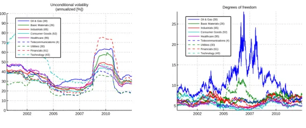
(nine industries). The left-hand side of Figure4displays the median values of the unconditional volatility of the GJR models over time, computed for each sector. The number within parentheses reports the number
of stocks for the industry (industry definition at the end of June 2012). We notice similar shapes for the unconditional volatility, except for the technology sector, which exhibits a substantially higher volatility
after the dot-com bubble. Further, the financial sector shows the highest volatility during the latest financial crisis. 2002 2005 2007 2010 0 10 20 30 40 50 60 70 80 90 100 Unconditional volatility (annualized [%]) Oil & Gas (30)
Basic Materials (26) Industrials (65) Consumer Goods (52) Healthcare (95) Telecommunications (4) Utilities (30) Financials (61) Technology (43) 2002 2005 2007 2010 5 10 15 20 25 Degrees of freedom Oil & Gas (30)
Basic Materials (26) Industrials (65) Consumer Goods (52) Healthcare (95) Telecommunications (4) Utilities (30) Financials (61) Technology (43)
Figure 4: Left: Median value of the estimated unconditional volatility per sector over time. Right: Median value of the estimated degrees-of-freedom parameters per sector over time.
The right-hand side of Figure4shows the median degrees-of-freedom parameter for each sector. We
notice a clear departure for the “Oil and Gas” sector, which has a smaller conditional kurtosis. In a similar
fashion to the previous section, the reason for this may be the relatively high volatility.
For persistence and leverage, the graphs look similar across industries (and hence similar to the
aggre-gate graphs in Section3.1).
3.3. Sizes
We now turn to the analysis with respect to the size of the stocks. To that end, at each time point, we
rank the 406 stocks with respect to the market capitalization at the fitting time, and form percentile groups. We compute the median values of the top (large cap), medium (mid cap) and bottom (small cap) groups,
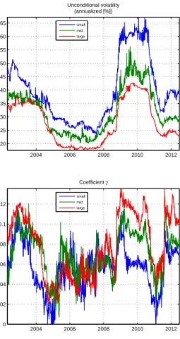
where each group consists of 40 equities. The top left-hand side of Figure5 displays the median values of the estimated unconditional volatility of the GJR models over time, computed for the three groups of
interest. We notice the common trends of the unconditional volatilities, with the clear feature that small cap stocks have a higher volatility than large cap stocks (on average 10% higher). Interestingly, during the latest
financial crisis the discrepancy between small and large cap stocks increases (on average 20% higher). The top right-hand side and bottom left-hand side of Figure5show that returns on small cap stocks have
a larger conditional kurtosis (lower degrees-of-freedom parameter) and a higher leverage effect (especially since the latest financial crisis) than mid cap and large cap stocks, and that (except for the different levels)
the patterns over time are somewhat similar across sizes. For persistence, the graphs look similar across sizes (and hence similar to the aggregate graph in section3.1).
In future research, we intend to investigate the following extensions. First, the symmetric Student-t distribution can be replaced by the skewed Student t distribution ofHansen (1994). Second, stocks of
different countries or continents can be considered instead of the S&P 500 constituents. Third, the time-varying behavior of the GJR model parameters can be explicitly described in a model. For this purpose,
one can consider a two-step estimation procedure similar to the approach ofDiebold and Li(2006) for the Nelson-Siegel model with time-varying parameters; in our context, one can estimate an AR, VAR or factor
model for the parameter estimates. Alternatively, the GJR model parameters and their dynamics can be simultaneously estimated in a non-linear, non-Gaussian state space model that is somewhat similar to the
models ofKoopman et al.(2010) orKoopman and Van der Wel(2011). Koopman et al.(2010) estimate a spline function of time for the parameter that makes the Nelson-Siegel model non-linear; a similar choice
2004 2006 2008 2010 2012 20 25 30 35 40 45 50 55 60 65 Unconditional volatility (annualized [%]) small mid large 2004 2006 2008 2010 2012 4 4.5 5 5.5 6 6.5 7 7.5 8 8.5 Degrees of freedom small mid large 2004 2006 2008 2010 2012 0 0.02 0.04 0.06 0.08 0.1 0.12 Coefficient γ small mid large
Figure 5: Top left: Median value of the estimated unconditional volatility per size over time. Top right: Median value of the estimated degrees-of-freedom parameters per size over time. Bottom left: Median value of the estimated leverage coefficients per size over time.
can also be investigated in our context.
References
Black, F., Jan.–Mar. 1976. The pricing of commodity contracts. Journal of Financial Economics 3 (1–2), 167–179.
Bollerslev, T., Apr. 1986. Generalized autoregressive conditional heteroskedasticity. Journal of Econometrics 31 (3), 307–327. Diebold, F. X., Li, C., 2006. Forecating the term structure of government bond yields. Journal of Econometrics 130 (2), 337–364. Glosten, L. R., Jaganathan, R., Runkle, D. E., Dec. 1993. On the relation between the expected value and the volatility of the
nominal excess return on stocks. Journal of Finance 48 (5), 1779–1801.
Hansen, B. E., 1994. Autoregressive conditional density estimation. International Economic Review 35 (3), 705–730.
Koopman, S. J., Mallee, M. I. P., Van der Wel, M., 2010. Analyzing the term structure of interest rates using the dynamic Nelson-Siegel model with time-varying parameters. Journal of Business and Economic Statistics 28, 329–343.
Koopman, S. J., Van der Wel, M., 2011. Forecasting the U.S. term structure of interest rates using a macroeconomic smooth dynamic factor model. Tinbergen Institute Discussion Paper TI 2011-063/4.
Lesmond, D. A., Ogden, Joseph, P., Trzinka, C. A., 1999. A new estimate of transaction costs. The Review of Financial Studies 12 (5), 1113–1141.
McNeil, A. J., Frey, R., Nov. 2000. Estimation of tail-related risk measures for heteroscedastic financial time series: an extreme value approach. Journal of Empirical Finance 7 (3–4), 271–300.