Panel Data Analysis of the Time-Varying Determinants of Corruption

Texte intégral

(1)2006s-28. Panel Data Analysis of the Time-Varying Determinants of Corruption Guillaume R. Fréchette. Série Scientifique Scientific Series. Montréal Décembre 2006. © 2006 Guillaume R. Fréchette. Tous droits réservés. All rights reserved. Reproduction partielle permise avec citation du document source, incluant la notice ©. Short sections may be quoted without explicit permission, if full credit, including © notice, is given to the source..

(2) CIRANO Le CIRANO est un organisme sans but lucratif constitué en vertu de la Loi des compagnies du Québec. Le financement de son infrastructure et de ses activités de recherche provient des cotisations de ses organisations-membres, d’une subvention d’infrastructure du Ministère du Développement économique et régional et de la Recherche, de même que des subventions et mandats obtenus par ses équipes de recherche. CIRANO is a private non-profit organization incorporated under the Québec Companies Act. Its infrastructure and research activities are funded through fees paid by member organizations, an infrastructure grant from the Ministère du Développement économique et régional et de la Recherche, and grants and research mandates obtained by its research teams. Les partenaires du CIRANO Partenaire majeur Ministère du Développement économique, de l’Innovation et de l’Exportation Partenaires corporatifs Alcan inc. Banque de développement du Canada Banque du Canada Banque Laurentienne du Canada Banque Nationale du Canada Banque Royale du Canada Banque Scotia Bell Canada BMO Groupe financier Bourse de Montréal Caisse de dépôt et placement du Québec DMR Conseil Fédération des caisses Desjardins du Québec Gaz de France Gaz Métro Hydro-Québec Industrie Canada Investissements PSP Ministère des Finances du Québec Raymond Chabot Grant Thornton State Street Global Advisors Transat A.T. Ville de Montréal Partenaires universitaires École Polytechnique de Montréal HEC Montréal McGill University Université Concordia Université de Montréal Université de Sherbrooke Université du Québec Université du Québec à Montréal Université Laval Le CIRANO collabore avec de nombreux centres et chaires de recherche universitaires dont on peut consulter la liste sur son site web. Les cahiers de la série scientifique (CS) visent à rendre accessibles des résultats de recherche effectuée au CIRANO afin de susciter échanges et commentaires. Ces cahiers sont écrits dans le style des publications scientifiques. Les idées et les opinions émises sont sous l’unique responsabilité des auteurs et ne représentent pas nécessairement les positions du CIRANO ou de ses partenaires. This paper presents research carried out at CIRANO and aims at encouraging discussion and comment. The observations and viewpoints expressed are the sole responsibility of the authors. They do not necessarily represent positions of CIRANO or its partners.. ISSN 1198-8177. Partenaire financier.

(3) Panel Data Analysis of the Time-Varying * Determinants of Corruption Guillaume R. Fréchette † Résumé / Abstract Depuis longtemps, des modèles sont utilisés dans le but de déterminer les causes de la corruption. Toutefois, l’analyse empirique demeure complexe. Qui plus est, les données sont difficiles à recueillir et couvrent souvent un nombre restreint de pays et une période limitée. Ce genre d’évaluation présente aussi des complexités inhérentes. Le présent document met l’accent sur le recours à des techniques de données de panels dans le but de mieux connaître les facteurs qui influent sur la corruption bureaucratique. En outre, cette analyse souligne le problème d’endogénéité qui ressort de l’analyse des causes de la corruption et propose une nouvelle variable instrumentale permettant de contrer celui-ci. Pour faciliter la démarche, ce document utilise un ensemble de données fournissant des renseignements sur au moins 135 pays et pour une période de seize ans. Les résultats indiquent que si le problème d’endogénéité n’est pas pris en compte, les résultats sont sérieusement biaisés. De plus, la corruption est décrite comme étant procyclique. Mots clés : corruption, endogénéité. There is a long history of models attempting to identify the causes of corruption, yet empirical analysis is complicated. Not only is data difficult to obtain and often available only for few countries and a limited number of years, but such estimation involves inherent complexities. This paper focuses on the use of panel data techniques to better identify factors that affect bureaucratic corruption. Furthermore, this paper identifies an endogeneity problem which arises in the analysis of the causes of corruption, and a new instrumental variable is proposed to solve it. To help in this endeavor, a data set is employed which provides information for as many as 135 countries over a span of sixteen years. Results show that neglecting the endogeneity problem leads to severely biased results. Using panel data techniques reveals that the availability of rents is a crucial determinant of corruption and that previous research may have underestimated the economic significance of rents on corruption. Furthermore, corruption is shown to be procyclical. Keywords: corruption, endogeneity, income, rents Codes JEL : H8, K4, C33. *. This paper has benefited from discussions with Rafael Di Tella, John Ham, David Hineline, Steven Lehrer, and John Kagel to whom I am very grateful. I also benefited from the help of Dilek Aykut and Daniel Treisman who provided me with data. I wish to thank Neil Bush, Lung-Fei Lee, Steve Leider, Dan Levin, Howard Marvel, Massimo Morelli, Jim Peck, Utku Unver, and seminar participants at the Corruption and Rent Seeking I session of the Public Choice 2001 meetings and participants of the Economics of Crime Prevention and Corruption session of the Canadian Economic Association 2001 meeting for helpful comments. My research was partially supported by the Center for Experimental Social Science, the C.V. Starr Center and the National Science Foundation (Grant SES-0519045). † CIRANO, email: guillaume.frechette@cirano.qc.ca and New York University, Department of Economics, 269 Mercer St. 7th Floor, New York, NY, 10003-6687, USA, email: frechette@nyu.edu.

(4) 1. Introduction. Bureaucratic corruption is an important phenomenon for many reasons. Corruption might depress investment which in turn reduces growth. It can also result in the misallocation of resources. Furthermore, lack of respect for public service can cause talented inidviduals to shy away from working for the government. Finally, it can a¤ect public …nances by making funds from the World Bank and the IMF unavailable. In recent years, these two institutions have decided to crack down on corruption by making funds contingent on e¤orts to eliminate corruption. This can have dramatic consequences on a country’s …nances and on its development. For instance, in 1997 the IMF suspended a $220 million loan to Kenya after its President failed to create a new anticorruption authority. Part of the focus of empirical work on corruption has been on the e¤ects of rents. Ades and Di Tella (1999) suggest that increasing competition in the bidder’s market has an ambiguous e¤ect. A decrease in rents due to increased competition reduces the incentives for bureaucrats to engage in corrupt practices. But this also reduces the incentives for the government to monitor them and prompts them to rewrite contracts, thus having the opposite e¤ect.1 This sets the stage for two empirical questions. First, does the availability of rents a¤ect the amount of corruption? Second, is this e¤ect positive or negative? One problem that arises is that one of the control variables, income, may be endogenous (see Treisman (2000)), which could bias the estimate of rent on corruption. In this paper I propose a new instrumental variable for income to re-evaluate the e¤ects of changes in rent (and other factors) on variation in corruption. The introduction of a time varying instrumental variable will solve the endogeneity problem even in the presence of unobserved country speci…c e¤ects. This paper will be concerned with variables that change over time, and since unobservable country speci…c e¤ects might be of great importance in this application, the paper will focus attention on …xede¤ects estimates.2 This raises a particular set of issues, such as concern for sample size, and limits the choice of instruments to time varying ones. This paper though, o¤ers solutions to these problems. The results suggest that accounting for endogeneity and country speci…c e¤ects as well as dealing with the endogeneity of income is crucial as it reveals that rents are more important than previous estimates 1 Earlier. models focussed on competition amongst bureaucrats, see for instance Rose-Ackerman (1978) and Schleifer and. Vishny (1993). 2 Results without country speci…c e¤ects are provided in the Appendix for reference. For a more detailed discussion go to http://homepages.nyu.edu/~gf35/print/frechette_corruption.pdf.. 1.

(5) have suggested – both in terms of statistical signi…cance and in terms of magnitude. Moreover, such an approach indicates that estimates of the e¤ect of income on corruption are severely biased downward if one doesn’t correct for its endogeneity. In fact, the e¤ect of income and education on corruption is found to be the opposite of what has been found in past studies. This implies that corruption is procyclical. Finally, political freedom is shown to have an important, and nonlinear, impact on corruption. A better understanding of the causes of corruption is critical to establishing more e¤ective policies aimed at its reduction. Also, determining the magnitude of the impact of di¤erent channels is important as this has a direct impact on the cost of alternative corruption reducing policies.. 2. Background, Data, and Methodology. The speci…cation used in this paper closely follows that of Ades and Di Tella (1999, hereafter AD). The reader interested in the details for the speci…c choice of regressors is referred to their paper. Another paper that is relevant to this study is that of Treisman (2000) who, to our knowledge, is the …rst to identify the potential endogeneity of income and to propose an instrument for it. Since his focus is mainly on the e¤ects of time-invariant factors such as religious or legal traditions, the focus is on cross-sectional analysis, and the instrument proposed does not vary over time. When he uses distance from the equator as an instrument for log per capita GDP, he …nds that this does not a¤ect the results. Without going any further in the details of previous works (for reviews of the literature see Elliott (1997), Jain (2001), and Mauro (1997)), let me summarize the most signi…cant results (at least for time varying variables): (1) higher income implies lower corruption, (2) a higher share of imports in GDP results in lower corruption, and (3) fewer political rights (fewer years of democracy) increase corruption. Result (1) is probably the most stable one, even when Treisman uses 2SLS and instruments for income using distance from the equator neither the sign nor the statistical signi…cance of the coe¢ cient estimate of income change. Result (2) is true even when AD uses 2SLS techniques to deal with the potential endogeneity of the share of imports in GDP. Treisman …nds support for this as well, although his results are not as stable. Finally, result (3) doesn’t seem robust to the use of …xed-e¤ects (hereafter FE). In both samples used by AD, when estimating FE, the coe¢ cient estimate on the lack of political rights variable becomes insigni…cant. On the other hand, Treisman consistently …nds support for the result that fewer political rights increase corruption. One other result worth mentioning is that Treisman …nds strong support for some of the other socio/historical factors he introduced, namely if the country is a former British colony and the percentage of Protestants. 2.

(6) As was previously mentioned, the focus of this paper will be on FE estimation, and there are many reasons for doing so. AD suggests that there may be country unobservables which are correlated to both rents and corruption. Certainly, as Treisman demonstrated, there are time-invariant factors that matter, and taking FE will account for these factors, even those not yest considered or those for which there is no data available. The reason I want to control for such unobservables is evident. Imagine for example that in some countries there is a culture of never telling on people, even if they broke the law. Clearly, if people do not talk about what others are doing, it fosters corruption by reducing the chances of getting caught. Furthermore, imagine that in countries where there are historically low rents, people tend to be less likely to denounce others and also suppose that, conditional on this cultural factor, rents decrease corruption. Then, if one regresses corruption on rents without conditioning on this cultural variable, you might get a negative coe¢ cient estimate on rents since you are confounding the e¤ects of rents and culture. Note also that this bias will be transmitted to all other regressors correlated with rent, even if they are not correlated with culture. One other appealing feature of FE is that it could solve the endogeneity problems. Note that there are two potential endogeneity problems: share of imports in GDP could be endogenous and so could income. If the endogeneity problems arise because of correlation with the country speci…c part of the error term, then estimating FE could resolve the estimation problem. There is evidence to support the position that country speci…c unobservables might be important in this application. In AD’s paper, FE yielded di¤erent results than OLS and 2SLS (both of which gave similar estimates). Finally, there is one more reason why one would want to use FE estimation. Subjective estimates of corruption might be a¤ected by preconceived ideas and biases. However, it seems likely that those a¤ect the level of the estimate but not the changes from one year to the next. If this is true, if despite misconceptions that could a¤ect the level of a country’s index, as long as the individuals who determine these indexes can determine changes in corruption correctly, then FE estimates would not be a¤ected by the incorrect level and would be the appropriate estimator. Similar to previous studies of this type, this paper will rely on a subjective measure of corruption. Hence, one might wonder how accurate or reliable such estimates are. Treisman provides a very complete and eloquent answer to this question which is only summarized here (the interested reader is referred to Treisman pp.410-412). First, these estimates tend to be highly correlated, which suggests that they are to some extent consistent. Second, they tend to be highly correlated with themselves across years, again suggesting that they are picking up something enduring.3 Third, someone might argue that the previous two 3 As. will be pointed out later, this is not to say that there is no variation. It is sometimes suggested that such index are. too noisy in the time dimension to take advantage of the panel structure of the data. The question, of course, is one of the. 3.

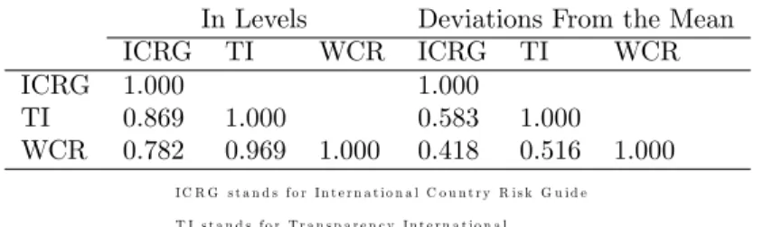
(7) ICRG TI WCR. ICRG 1.000 0.869 0.782. In Levels TI WCR 1.000 0.969. 1.000. Deviations From the Mean ICRG TI WCR 1.000 0.583 1.000 0.418 0.516 1.000. IC R G sta n d s fo r Inte rn a tio n a l C o u ntry R isk G u id e T I sta n d s fo r Tra n sp a re n c y Inte rn a tio n a l W C R sta n d s fo r W o rld C o m p e titive n e ss R e p o rt. Table 1: Correlation Between Corruption Indexes For Overlapping Countries and Years (1996-1997) arguments are simply by-products of the fact that these estimates are in‡uenced by biases and stereotypes. Nonetheless, as Mauro 1995 shows, corruption, or the subjective estimates of corruption, seem to negatively a¤ect economic growth by depressing investments. Thus, even if these rankings are a¤ected by perceptions, these perceptions have real e¤ects. Two other justi…cations of a more technical nature which I would propose are the following. First, as mentioned earlier, even if the levels of these indixes were a¤ected by misconceptions, as long as changes from those levels are correct, a FE estimator will result in unbiased estimates. Furthermore, even if these are imperfect measures, if the errors are what is often referred to as classical (mean zero and uncorrelated with the true corruption) then the estimates would be unbiased since such errors are uncorrelated with the regressors. The speci…c index I will use is that of the International Country Report Guide (hereafter ICRG).4 To my knowledge, the ICRG data set has not been used previously to study the causes of corruption.5 The ICRG index is highly correlated with the indexes used by Treisman as is shown in Table 1 (and to the WCR index used by AD).6 Furthermore, considering deviations from their mean, which is what FE does, the ICRG data importance of the signal to noise ratio. As I will show, our estimates indicate statistically signi…cant results, some of which are robust across speci…cations. This cannot result from changes simply due to noise. Furthermore, these do not follow simple trends since including the year as a regressor in the OLS and IV speci…cations always resulted in that regressor being statistically insigni…cant. 4 The ICRG corruption index ranges from zero to six. It is reported on a monthly basis, but I am using annual averages. This means that for practical purposes, it is continuous between zero and six. Lower scores indicate “high government o¢ cials are likely to demand special payments”and that “illegal payments are generally expected throughout lower levels of government”in the form of “bribes connected with import and export licenses, exchange controls, tax assessment, police protection, or loans.” For purposes of comparability, I have transformed the variable such that zero is the lowest degree of corruption and higher numbers indicate greater corruption. It is also rescaled to range from zero to ten to make results comparable to previous works. 5 Although it is considered by Treisman, he decides not to use it because he points out some scores which he …nds suspicious. Although I will not argue that the speci…c examples he gives are not suspicious, I will argue that these must be exceptions. 6 The countries and years used for each index are reported in the Appendix.. 4.

(8) is more correlated with Treisman’s main index (TI) than with one of the data sets used by AD (WCR) as illustrated in Table 1. The ICRG data also meets the criterion of high correlation across years exhibiting correlations of at least 0.941 from one year to the next.7 Thus, even if there are anomalies, they are most likely to be exceptions and, as previously noted, if these errors are classical, should not bias the results. However, the main reason for using the ICRG data is that it is considerably larger than any alternative data sets; it covers 135 countries for as long as sixteen years.8 Although sample size may not be crucial for all estimators, it is certainly of importance when one uses IV techniques as I will do. The 2SLS’s bias decreases with sample size, and even though it is not clear how many observations are required for the estimates to stabilize, more is de…nitely better. The rest of the data used is similar to that of AD except that in order to focus on FE, only time varying regressors will be used. Schooling is measured as the ratio of total enrollment in primary school, regardless of age, to the population of the age group that o¢ cially corresponds to the primary school level.9 Estimates are based on the International Standard Classi…cation of Education. Income is GDP per capita divided by 1000. Political freedom is given by the Gastil index of political rights. The Gastil index ranges from one to seven, one being the highest degree of political freedom. Every estimated equation will have as two of its regressors ‘high political freedom’and ‘lack of political freedom.’ High political freedom is an indicator variable taking value one if the Gastil index is less than or equal to three. Lack of political freedom is an indicator variable taking value one if the Gastil index is greater than or equal to six. Thus the excluded values are four and …ve. Note that this departs from the AD speci…cation which included the Gastil index as a regressor. However, using the Gastil index directly assumes that the e¤ect of political freedom on corruption is the same going from a score of one to two as going from a score of six to seven. Of course this may not be the case and permitting all these scores to enter as a set of seven indicator variables allows for nonlinear e¤ects. It turns out that the hypothesis that the e¤ect is the same for scores one, two and three, the same for scores four and …ve, and that the e¤ect for scores six and seven is the same cannot be rejected for the crucial regressions (a more detailed analysis of the e¤ects will be o¤ered in the discussion of the results). Thus these are grouped for ease of exposition. The level of pro…ts is accounted for by the share of merchandise imports in GDP and the fraction of fuel and mineral exports in the total exports of goods and services (which will often be 7 This. is not to say that there is no variation over time in the data. On average, countries scores vary by 23% between their. highest and lowest levels. 8 Note that not all the countries are in the data set for all sixteen years. For instance, there were ninety countries in 1982. 9 This was preferred to AD’s measure because it varies over time.. 5.

(9) referred to simply as share of fuel and mineral exports)10 . Two instruments will be used, one to control for the potential endogeneity of share of imports in GDP and the other for income. The instrument for share of import in GDP is one of the two proposed by AD, log of population, which is obtained from the World Development Indicators.11 As for income I propose a new instrument which is presented bellow. Treisman was the …rst to identify this potential problem and to suggest an instrument. Although he found no evidence that such a correction mattered, this lack of evidence could be speci…c to the data set or to the instrument.12 The new instrument, which will be explained in more detail, is the per capita GDP of a country’s greatest importer for the mid-sample year of 1989,13 and this will be used as an IV for income. This is constructed in part using data from the Direction of trade statistics which is published by the IMF. This source gives me the country which is the greatest importer for each country in our data. The complete data sources are provided in the Appendix. The remainder of this paper will be organized as follows. First, the instruments and …rst-stage regressions are presented. Then I cover the analysis of the determinants of corruption. Finally, the results are discussed and interpreted.. 3. First-Stage Regressions: the Instruments. To correct for endogeneity problems, I will use two methods. First, if the regressors causing problems can be decomposed into a permanent or time-invariant part and a part that varies over time, and the endogeneity 1 0 Note. that this di¤ers from AD’s measure of rents through exports. They take the percentage of fuel, mineral, and metals. export in merchandise exports whereas I use the percentage of fuel, ores, and metals export in total exports of goods and services. This is done for two reasons. First, I believe this better captures the importance of rents as merchandise exports may be a negligible portion of all exports for some countries, thus these rents would be of no relevance. It also improves the statistical signi…cance of the estimates for this coe¢ cient without a¤ecting others. This last claim will be elaborated on in the discussion. Note that since the data given to the World Bank for fuel and mineral exports and exports of goods and services are from di¤erent sources, there are a few observations that are inconsistent (the former is greater than the latter). These were simply dropped. This a¤ected only twenty observations or only about 2% of the data. 1 1 I do not use the other one they propose, land area, since it does not vary over time. 1 2 Most of the empirical literature on corruption deals with the e¤ect of corruption on growth. For instance, Shleifer and Vishny (1993) argue that corruption reduces growth. The same argument is made by Mauro (1995) who suggests in his empirical study that corruption reduces investment which in turn reduces growth. Of course, growth and income are di¤erent, but they are correlated. In a FE context, the interest is in deviations from the mean. 1 3 The choice of year is arbitrary, but there is no reason to believe it a¤ected the results. There are a few exceptions to this, and these are all noted in the Appendix.. 6.

(10) results only from the permanent part, then FE will solve this problem. To see this, denote corruption and income at time t for country i: Cit and Yit . Let’s suppose that Cit = cli + cit and Yit = yli + yit , where cli and yli are country speci…c corruption and income levels. Assume that the true relationships are (1) Cit =. + (yli + yit ) + "it and (2) yli =. + cli +. i.. Simply estimating OLS on the corruption. equation would not yield consistent estimates since the right hand side determines the left hand side (in (1)) but part of the right hand side is also simultaneously determined by the left hand side (from (2)). Instead, one can estimate the corruption equation using OLS on the di¤erences from the mean (i.e. take P P P FE): Cit (yli + yit (yit T T Cit = T (yli + yit )) + it = T yit )) + it . It is easy to see that this transformation eliminates the endogeneity problem that is present if one simply estimate OLS, since yli. is eliminated from the right hand side. Of course, there are other reasons to use FE which are valid even if there is no endogeneity problem, for instance, to correct for unobserved time invariant factors. However the endogeneity may not take the particular form illustrated above. Consequently, another way to solve this problem is used, namely instrumental variable techniques. A valid instrument is one such that the instrument is uncorrelated with the error term in the equation of interest (the second-stage regression) and it has some partial correlation with the endogenous regressor (in the …rst-stage regression). Note that when estimating FE and IV simultaneously, a valid instrument needs to be rede…ned in terms of the deviations from the mean. The endogeneity of the share of imports in GDP has been recognized earlier, when AD suggested it as a proxy for rents (Ades and Di Tella 1999).14 Clearly bureaucrats can a¤ect imports; therefore their corruption can both determine and result from the share of imports in GDP. The instrument used here is the same as the one used by Ades and Di Tella (1999), the natural log of population. There is no a priori reason why one would expect population to a¤ect corruption, and to my knowledge, no model of corruption suggests that it should depend on population. On the other hand, the e¤ect of population on foreign trade as a portion of GDP is a well established phenomenon. For instance, Perkins and Syrquin (1989) write “the one proposition that is beyond dispute: the larger a nation’s population, the lower is the share of foreign trade in that nation’s GDP.”(p. 1705.) Multiple explanations for this relationship are suggested, including: transport cost favoring domestic producers in large countries, economies of scale enjoyed by large countries, distribution of mineral resources around the globe (small nations have more than they can use at home), and others. In this case however, the variable of interest is not the share of foreign trade in that nation’s GDP but a subset of foreign trade, namely imports. Nonetheless, since imports and foreign trade are positively 1 4 This. was also noted by Treisman (2000): “corrupt o¢ cials may themselves create barriers to imports.” p. 408.. 7.

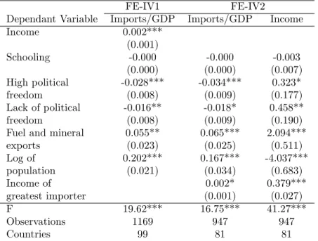
(11) correlated, the result almost certainly extends (that it does will be shown below).15 For instance, in the context of analyzing the determinants of growth, Levine and Renelt (1992) conclude that “all …ndings using share of exports in GDP could be obtained almost identically using the total trade or import share” (p. 959). If it is di¢ cult to understand why population levels and corruption would be correlated, it is even more di¢ cult to see why variations in population (around a country’s average population) would correlate with changes in corruption. This is to say that in FE, it seems unlikely that population is not exogenous in the second stage equation. The …rst column of Table 2 shows the estimates for imports over GDP as a function of (log) population and other regressors conditional on country FE (labelled FE-IV1). Note that population seems to provide a strong instrument as the F statistic is above the Staiger and Stock (1997) rule of thumb threshold for weak instruments,16 and the coe¢ cient estimate on (log) population is highly statistically signi…cant, the negative sign, as compared to the previous case. This could be explained if after an increase in the demand in a country, most of the extra demand is ful…lled in the short-run by supply from the rest of the world. This implies that the share of imports in GDP is counter-cyclical. This result is not surprising. When income grows, holding population constant, if not all of the increased demand goes to imports (some of it goes toward domestic production), then the numerator of the left-hand side variable increases by less than the denominator. The coe¢ cient estimate on political freedom implies that when political freedom changes in a country, it increases imports as a share of GDP when it goes toward an intermediate level of political freedom. Finally, the share of fuel and mineral exports in total exports moves in the same direction as the share of imports in GDP. However, this paper also proposes to control for the endogeneity of income. Thus far, the …rst stage regression presented would apply if only share as a fraction of income was endogenous. This was provided to allow comparison to Ades and Di Tella’s (1999) work and to give a point of comparison to see the e¤ect of allowing and controlling for the endogeneity of income. Here is a description of how I propose to identify the e¤ect of income on corruption. There is little doubt that, over time, a country’s per capita GDP is correlated with the per capita GDP of the country to which it sells most of its exports. Note that since this paper focuses on FE estimates, the correlation needs to come from the changes in per capita GDP, not from 1 5 To. see why this make sense, take the special case where current-account balance equals net investment income from. nonresidents, then exports has to equal imports. 1 6 Staiger and Stock (1997) argue that when there is only one endogenous variable, instruments should be deemed weak if the …rst stage F statistic is less than ten.. 8.

(12) Dependant Variable Income Schooling High political freedom Lack of political freedom Fuel and mineral exports Log of population Income of greatest importer F Observations Countries. FE-IV1 Imports/GDP 0.002*** (0.001) -0.000 (0.000) -0.028*** (0.008) -0.016** (0.008) 0.055** (0.023) 0.202*** (0.021). 19.62*** 1169 99. FE-IV2 Imports/GDP Income. -0.000 (0.000) -0.034*** (0.009) -0.018* (0.009) 0.065*** (0.025) 0.167*** (0.034) 0.002* (0.001) 16.75*** 947 81. -0.003 (0.007) 0.323* (0.177) 0.458** (0.190) 2.094*** (0.511) -4.037*** (0.683) 0.379*** (0.027) 41.27*** 947 81. Standard errors in parenthesis (clustered std. errors in OLS, IV1, and IV2). ***,**,* indicate statistical signi…cance at the 1%, 5%, and 10% level respectively.. Table 2: First Stage Estimates (Imports/GDP and Income endogenous) the levels of GDP. In other words, it’s not that rich (poor) countries export to rich (poor) countries –or vice versa –but rather that when the country to which you export the most is getting richer, it is likely to make you richer as well. The reasoning is quite simple. Variations in income are in part a¤ected by variations in demand, and an important part of those variations in demand are determined by the changes in income of the country which buys the most of another country’s exports. On the other hand, there is no reason to believe that the changes in (or level of) income of the country to which you export the most are correlated to the changes in your corruption levels. In order for this not to be true, changes in corruption of many countries would need to correlate to the changes in income of very few countries. For instance, over half the countries in this sample have one of three countries as their main export destination. To take a concrete example, even though Bangladesh and England both have the United States as their greatest export destination, the evolution of corruption in each of those countries followed very di¤erent paths. Thus, turning to the …rst stage regressions under the FE-IV2 heading in Table 2, one notes that again, for the Imports/GDP regressions, the results are similar in terms of sign, magnitude, and statistical signi…cance as in the FE-IV1 case. However, income of greatest importer yields a small positive estimate (as opposed. 9.

(13) to small negative for income in FE-IV1). In the Income regression, schooling is not statistically signi…cant, which could be explained if it takes a long time for education to have an impact on income. Political freedom once again exhibits a non-linear relation, but it is the opposite than in the Imports/GDP regressions. That is, ceteris paribus, either reducing or increasing political freedom away from its intermediate level would increase income. Fuel and mineral exports as a share of total exports has a positive impact on income, which is easy to rationalize since increasing exports of a natural resource in the short-run must increase income. The instrument, (log) population, is also highly statistically signi…cant and has the expected sign, reproducing the result that larger countries have a lower share of imports in GDP. But furthermore, it has been argued before that high population growth is likely to lead to a decrease in per capita income if the rate of technological growth is not high enough (Enke 1971). Finally, as expected, income of greatest importer has a positive and highly statistically signi…cant impact on income. Moreover, both instruments are statistically signi…cant in both regressions, and the F statistic soundly rejects the insigni…cance of the …rst stage regressions. Hence, population and income of the greatest importer have been shown to be valid instruments for share of imports in GDP and income controlling for country …xed e¤ects. That is to say that changes in population and income of the greatest importer are orthogonal to the residuals in a corruption equation. Furthermore, explanations for their correlation with and evidence that they are partially correlated with share of imports in GDP and income are o¤ered. But is there a need to perform such a correction, i.e. are share of imports in GDP and income endogenous? Using a Durbin-Wu-Hausman type test suggested by Davidson and MacKinnon (1993), the null hypothesis that these two regressors are exogenous can be rejected at any conventional level.17 One additional concern however could be that when both instruments are used, the instrumented variables for income and share of imports in GDP do not have enough variation (multicolinearity). Fortunately, this does not seem to be cause for concern in this case, as the correlation between the predicted values in FE-IV2 is 0.448.18. 10.

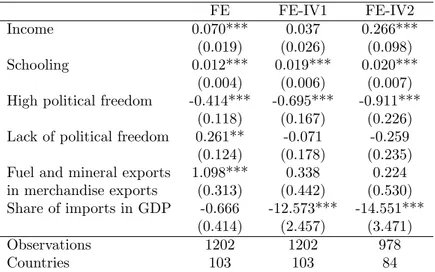
(14) Income Schooling High political freedom Lack of political freedom Fuel and mineral exports Share of imports in GDP Observations Countries. FE 0.072*** (0.019) 0.011** (0.004) -0.447*** (0.119) 0.282** (0.124) 1.346*** (0.342) -0.832* (0.458) 1169 99. FE-IV1 0.049** (0.024) 0.013** (0.006) -0.762*** (0.157) -0.014 (0.162) 1.219*** (0.420) -11.415*** (1.975) 1169 99. FE-IV2 0.205*** (0.075) 0.012* (0.006) -0.952*** (0.199) -0.159 (0.198) 1.095** (0.462) -12.626*** (2.576) 947 81. Standard errors in parenthesis. ***,**,* indicate statistical signi…cance at the 1%, 5%, and 10% level respectively.. Table 3: The Determinants of Corruption (ICRG: 1982-1997). 4. Second Stage Regressions: The Determinants of Corruption. Table 3 presents the results for FE estimates, where FE-IV1 are estimates, the share of imports in GDP is instrumented and FE-IV2 are estimates where not only share of imports in GDP is instrumented but income as well.19 Income is positive, meaning that when income goes up, corruption increases as well. When income is instrumented, its coe¢ cient estimate increases. Schooling is positive in all regressions, which means that when the population becomes more educated, corruption increases. High political freedom has a negative estimate, hence increasing political freedom from the baseline of a Gastil index of four or …ve to three or less leads to a decrease in corruption. The coe¢ cient estimate on the e¤ect of fuel and mineral exports is positive, and thus a reduction in the importance of fuel and mineral exports as part of all exports implies a decrease in corruption. Share of imports in GDP is positive, and thus when imports become more important, relative to GDP, corruption decreases. Note that in both speci…cations where the endogeneity of share of imports is taken into account, the coe¢ cient estimate for share of imports in GDP is substantially higher, 1 7 Davidson 1 8 Note. and MacKinnon 1993, p. 237-240. that both instruments need to be used in both …rst stage regressions for consistency. Given that the instruments meet. the required assumptions, 2SLS is known to give consistent estimates (see for instance Chapter 5.2.1 of Wooldridge 2002). 1 9 Throughout the paper FE will be used interchangeably to mean the speci…c FE regression reported in the second column of Table 3 or the set of estimations (FE, FE-IV1, and FE-IV2) that rely on …xed e¤ects techniques.. 11.

(15) more than thirteen times greater than in the FE speci…cation. The e¤ect of correcting for the endogeneity of both income and share of imports in GDP is also noticeable in other coe¢ cient estimates, such as that for high political freedom and fuel and mineral exports which both increase. The coe¢ cient estimate for high political freedom more than doubles between the FE speci…cation and the FE-IV2 speci…cation. The only regressor which changes sign, and is only statistically signi…cant once, is lack of political freedom. It is only statistically signi…cant in the FE speci…cation, in which case it is positive, i.e., fewer political rights increase corruption. It is negative in the other two regressions, implying that a lack of political freedom, as compared to the baseline, reduces corruption. In all three speci…cations, an F test strongly rejects the null hypothesis that the country speci…c e¤ects are equal. It is worth noting that if country FE were not included, the results would di¤er in the following way. First, the coe¢ cient estimates of income and schooling all change signs, going from negative without FE to positive with FE. Second, using both FE and IV methods jointly has a considerable impact on the magnitude of some of the coe¢ cient estimates, namely share of imports but also high political freedom and fuel and mineral exports. Using either FE or IV by itself does not have such a dramatic impact.. 5. Discussion. Although some of the results support past research, others are quite di¤erent. As with previous papers, these results support the idea that higher rents increase corruption. But unlike previous papers, this e¤ect is found not only through share of imports in GDP but also through share of fuel and mineral exports in total exports. In fact, share of fuel and mineral exports in total exports is statistically signi…cant in the three speci…cations considered. This is an interesting …nding since fuel and mineral exports are less likely than share of imports in GDP to be endogenous, it gives stronger support to the hypothesis that rents a¤ect (positively) corruption. One potential criticism of this …nding is that evaluators are biased against “oil exporting countries” and simply assume that those are more corrupt. Such a critique seems less convincing given that the estimates are statistically signi…cant in the FE speci…cations, where such bias can be absorbed in the country speci…c e¤ect. To give an idea of the importance of the implied e¤ect of the coe¢ cient estimates, which are all slightly greater than one, consider the following. Increasing a country’s share of fuel and mineral exports in total exports by the sample standard deviation of 0.248,20 which predicts a change in the corruption ‘score’of 0.272, is approximately the di¤erence between Belgium’s average corruption of 1.211 and Australia’s average 2 0 This. is computed using the sample of 947 observations used in the FE-IV2 estimation.. 12.

(16) score of 1.510. It corresponds to about 0.116 standard deviation in the corruption index. This does not seem to be a very strong e¤ect in terms of magnitude, although some countries are clearly outliers in terms of how important fuel and mineral exports are to their economy. Note that, coincidentally, of the two FE estimations performed by AD, one of them yielded a positive coe¢ cient estimate on fuel and mineral exports. There are three potential explanations for this new result that fuel and mineral exports are statistically signi…cant. It could be the source of the data: ICRG versus other indexes. Another possibility is that a large amount of data is required to estimate this e¤ect, at least more data than used by previous studies. Finally, this could be due to the fact that fuel and mineral exports is de…ned as the share in exports of goods and services instead of the share in merchandise exports: i.e. the former is a better proxy for rents than the latter. To attempt determining which of these explanations is the correct one the estimation is performed with fuel and mineral exports in merchandise exports (see Table 8 in the Appendix). Note that almost all results are identical (qualitatively). This suggests that the source of the di¤erences is not the data set. However, the coe¢ cient estimate on fuel and mineral exports is now statistically signi…cant in only one speci…cation even though the sample size has not changed. This indicates that fuel and mineral exports in exports of goods and services is a better proxy of the relevant rents. The results for share of imports in GDP are consistent with previous studies that …nd most estimates are statistically signi…cant and negative. However, combining FE and IV yields lower coe¢ cient estimates. Note that this is true both in terms of the FE-IV estimates of this paper as compared to other estimates in this paper, and as compared to estimates of other papers except for one of AD’s FE estimates. AD’s estimates are between -1.871 and –12.73 (-2.405 if you exclude the one outlier estimate), and Treisman has estimates between -0.01 and -0.02. How important is an estimate of -12.626? A change of one standard deviation in the share of imports in GDP (the standard deviation is 0.232) implies a change in corruption of -2.925. This is clearly an important e¤ect. It represents over one quarter of the range of possible values (the measure of corruption takes values between zero and ten). It represents a change of 1.181 times the standard deviation of the corruption index. For the sake of illustration, this would be similar to the di¤erence in average corruption between the United Kingdom (1.073) and Brazil (3.875). But what can explain the coe¢ cient changing so much only after FE and IV are combined? This suggests that the endogeneity is really at the level of changes in the import share of GDP rather than at its level. In other words, the kind of endogeneity for which FE is a solution (see the …rst paragraph of the section First-Stage Regressions: the Instruments) is exactly what is not at work in this case. If you add to this the fact that country FE are important and correlated to the share of imports in GDP, you can get a situation where combining FE and 13.

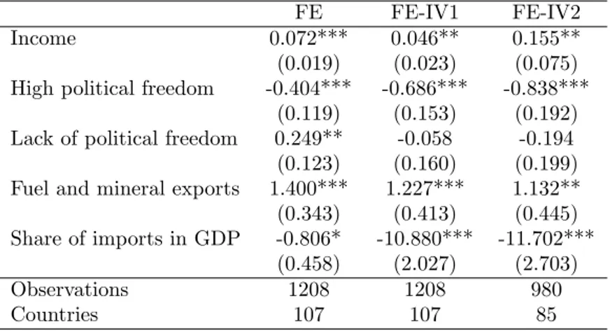
(17) IV gives di¤erent results from using either one by itself. The analysis of the e¤ects of income on corruption yields truly novel results. Controlling for the endogeneity of income increases its coe¢ cient estimate independently of the estimation method. This is entirely consistent with the source of the endogeneity, namely that corruption has a negative impact on income. AD had a similar result for their FE estimation in which they had a positive and statistically signi…cant estimate of the coe¢ cient of income for one of their two data sets (all other estimates of both AD and Treisman were negative).21 The estimates suggest that income has very important e¤ects on corruption. Once again, taking a change in income of one standard deviation (the standard deviation of income is 8.949) yields a change in corruption of 1.832. Again this is important as it represents slightly more than three quarters of a standard deviation in the corruption index or almost one …fth of the range of possible corruption scores. Thus the e¤ect could be compared to going from the average level of corruption of Mexico, 5.375, to the level of Gabon, 7.222. Corruption being procyclical is not implausible. In economic upturns, it might be that rents are generally increasing (besides what is captured by the import share of GDP and the share of fuel and mineral exports in total exports). This could be the result of the procyclical nature of labor productivity (Aizcorbe 1992). If the two proxies for rents used in this paper do not capture all the relevant rents, which is highly plausible, than this would explain the positive coe¢ cient estimate. The only prior study that estimates the e¤ect of schooling on corruption is that of AD, and they only do so in their OLS and IV speci…cations. Surprisingly all the coe¢ cient estimates of schooling are positive and statistically signi…cant. What can explain a positive coe¢ cient estimate on the estimate of the e¤ect of schooling? This cannot be established from this data set, but one possibility is that as the population is getting more educated, and thus better at controlling its bureaucracy, bureaucrats are also becoming more educated and thus better at performing corrupt acts. If bureaucrats are getting better faster than the population is improving its monitoring capability, this could explain the positive sign. A more plausible explanation however is that changes in schooling, as measured here, is more of a proxy for changes in rent than anything else. Figure 1 graphs the standard deviation of the measure of schooling against average income (the points are labelled by their World Bank country code). Clearly, for most developed countries, this variable barely changes in the entire sample. Consequently most of the variation in this variable comes 2 1 This. does con‡ict however with Treisman’s …nding that instrumenting for income doesn’t a¤ect the results. This di¤erence. is investigated further in the longer version of this paper. It is illustrated that sample size, choice of instruments, and/or the combination of FE and IV techniques are the driving force behind this di¤erence. The interested reader is referred to http://homepages.nyu.edu/~gf35/print/frechette_corruption.pdf.. 14.

(18) Standard Deviation of Schooling 20 30 10 0. MWI. UGA. HT I. KWT. AGO SUR DOM BRA PAK IRL NGA COG MOZ ZAR ZAF SLV MNG MDG ZWE MAR TMLI GO KEN T ZA EGY GIN GT M CMR LBN CYP BGD IRN ET H ZMB SGP ROM GAB GUY SEN BGR GBR GMB PNG BOL SAU CHN DZA T UR GNB VNM HKG ARE YEM OMN BFA RUS SLE TCOL HA BRN KOR NIC NZL GRC SDN ARG SYR BWA ECU CIV NAM HUN ISR NCL AUS IND GHA PRY ALB LKA MYS TPER UN PHL PRT IT A CHL BHR MEX HND CRI BHS VEN URY JAM CAN JOR POL IDN YUG NER PAN T CZE T O MLT ESP SVK. 0. 10. 20. CHE NLD SWE DEU FRA FIN USA AUT NORDNK BEL ISL. LUX. JPN. 30 Mean Income (x1000). 40. Figure 1: Relation Between Income and Changes in Schooling. from countries with relatively low income. In such countries, increases in the quantity of students is strongly a¤ected by foreign aid,22 but changes in foreign aid are a¤ecting the opportunities for corrupt behavior. This is particularly true given that aid has been documented to be fungible (World Bank 1998, pp. 60-74). Thus, the schooling variable might re‡ect something di¤erent than the e¤ect of schooling in its variation over time. To make sure other results are not driven by the schooling variable, the estimation is performed without it. It reveals almost identical results which are reported in the Appendix. Thus, if one is uncomfortable with this measure of schooling, the remaining results appear not to be a¤ected by it. Finally lets turn to political freedom. Clearly results indicate that the e¤ects of political freedom are nonlinear. This might explain why AD found lack of political rights to be rarely signi…cant (remember that they include the Gastil index directly as a regressor). In their own words, “Throughout this paper we fail to …nd bene…cial and signi…cant e¤ects of political rights on corruption. If anything, lack of political rights seems to be associated with less corruption” (AD, p. 987). However, Treisman consistently found that 2 2 See. for instance Pack and Pack (1990) which establishes a positive relation between aid and education (amongst other. things). Also see Assessing Aid – What Works, What Doesn’t, and Why (1998) from the World Bank: “Most aid is delivered as investment projects in particular sectors such as roads, water supply, or education.” p. 3.. 15.

(19) uninterrupted democracy resulted in lower corruption. The results presented here are not in contradiction with these earlier results. The insight is that this relation is nonlinear. Going from no political freedom to some is not enough: what is really bene…cial is to go one step further to a high degree of political freedom.23 Interpreting the magnitude of the results is simple. Going from a Gastil score of four or …ve to one of less than four implies a decrease in corruption of 0.952 points. For example, this would approximately correspond to the di¤erence in mean corruption between Kenya which has a score of 5.000 and Argentina at 4.111. One may be worried about the e¤ect of pooling scores together. As mentioned earlier, the joint hypothesis that the e¤ect of scores one through three is the same, that scores four and …ve have the same e¤ect, and that scores six and seven have the same e¤ect cannot be rejected for the crucial speci…cations FE-IV1 and FE-IV2 at any conventional levels (as for the FE estimates, the probability of rejection is 0.041). More importantly, for all speci…cations, results are qualitatively the same (there are no sign changes for instance). The estimates with one dummy for each level (except level four) are reported in the Appendix for completeness.. 6. Conclusion. The results presented in this paper con…rm some of the previous conclusions regarding the causes of corruption, but it also sheds light on some new results and raises entirely new questions. One result that is con…rmed is that rents foster corruption (This was shown mainly in AD but was also present to a lesser extent in Treisman.). Two new aspects of this relationship are presented in this paper. First, the e¤ect of rents on corruption can be found not only through the e¤ect of share of imports in GDP but also in the e¤ect of fuel and mineral exports. This e¤ect is found to be relatively small in magnitude and that may explain why it did not tend to be statistically signi…cant when using smaller data sets. Second, the e¤ect of share of imports in GDP may be much more important than was previously believed. The joint use of FE and IV techniques, to control for both country unobservables and endogeneity problems, reveals a coe¢ cient estimate which is many times larger than when these corrections are not performed. The use of a time varying measure of education permits analysis of the e¤ects of schooling in FE type speci…cations. These reveal that contrary to what OLS suggests, an increase in schooling may increase corruption. However, as previously noted, variations in this measure of schooling may be picking up something else. Another result which is con…rmed here is that greater political freedom decreases corruption (this found support mainly in 2 3 Looking. for evidence of an “inverted U pattern on the relation between democracy and rent seeking,” which is predicted. by their model, Mohtadi and Roe (2003) also observe that corruption and democracy exhibit a nonlinear relation (inverted U).. 16.

(20) Treisman, whereas AD had mixed results.). A new aspect of this result however, is that the relation between political freedom and corruption seems to be nonlinear. Finally, an entirely new …nding is that increases in income may not decrease corruption but might even increase it! As was explained in this paper however, this is entirely consistent with the endogeneity problem intrinsic in the relation between income and corruption. Furthermore, the procyclical nature of corruption is not counter intuitive once one considers the relation between factors such as productivity and income. Identi…cation of these new results relied on the use of FE and IV techniques. The former restricts the set of questions that can be asked, and thus there is no doubt that cross-sectional analysis is, for some questions, a better approach. For instance, most of the questions asked in Treisman cannot be considered within this framework. However, to analyze time-varying causes of corruption, such an approach has distinct advantages. The latter is restrictive in that it requires more observations to achieve reliable results and thus limits the choice of data set. Nonetheless, as was argued in this paper, although the ICRG data might not be perfect, it is nonetheless very similar to the other data sets that have been used in determining the causes of corruption. Clearly, one always wants to be cautious in interpreting such results, and eventually there will be enough data sets of substantial size to clarify this issue. The instrument proposed in this paper to control for the endogeneity of income performed very well. This instrument has several attractive features: it is easy to construct; it is not limited to any speci…c data set; and it varies over time. It seems plausible that it could be used in other applications investigating the causes of some social factor where income is both a cause and a consequence. The apparent importance of allowing for country speci…c e¤ects suggests that corruption might be imbedded in the bureaucratic and legal culture of a country in some signi…cant way. Just as Ades and Di Tella suggest that di¤erent individuals may be more or less willing to be corrupted, di¤erent countries’bureaucracies may be more tolerant of corruption. This appears true given the result of past research such as that of La Porta et al. 1998 and Treisman 2000. And although this could mean that the way out of corruption may be a long road for some countries, the importance of the e¤ect of share of imports in GDP on corruption might suggest that there are policy variables that can substantially decrease bureaucratic corruption. However, the …nding that increasing income and education increases corruption suggests that some policy objectives might work against each other.. 17.

(21) References Ades, A. and Tella, R. D.: 1999, Rents, competition, and corruption, The American Economic Review 89, 982–993. Aizcorbe, A. M.: 1992, Procyclical labour productivity, increasing returns to labour and labour hoarding in car assembly plant employment, The Economic Journal 102(413), 860–873. Davidson, R. and McKinnon, J. G.: 1993, Estimation and Inference in Econometrics, Oxford University Press, New York. Elliott, K. A. (ed.): 1997, Corruption and the Global Economy, Institute for International Economics, Washington, DC. Enke, S.: 1971, Economic consequences of rapid population growth, The Economic Journal 81(324), 37–57. Jain, A. K.: 2001, Corruption: A review, Journal of Economic Survey 15(1), 71–121. La-Porta, R., de Silanes, F. L., Shleifer, A. and Vishny, R. W.: 1998, Law and …nance, Journal of Political Economy 106, 1113–1155. Levine, R. and Renelt, D.: 1992, A sensitivity analysis of cross-country growth regressions, The American Economic Review 82(4), 942–963. Mauro, P.: 1995, Corruption and growth, The Quarterly Journal of Economics 110(3), 681–712. Mauro, P.: 1997, Corruption and the Global Economy, Institute for International Economics, Washington, DC, chapter The E¤ects of Corruption on Growth, Investment, and Government Expenditure: A CrossCountry Analysis. Mohtadi, H. and Roe, T. L.: 2003, Democracy, rent seeking, public spending and growth, Journal of Public Economics 87, 445–466. Pack, H. and Pack, J. R.: 1990, Is foreign aid fungible? the case of indonesia, The Economic Journal 100(399), 188–194. Perkins, D. H. and Syrquin, M.: 1989, Large Countries: The In‡uence of Size, Elsevier Science Publishers. Rose-Ackerman, S.: 1978, Corruption: A Study of Political Economy, Academic Press, New York. 18.

(22) Shleifer, A. and Vishny, R.: 1993, Corruption, The Quarterly Journal of Economics CIX, 588–617. Staiger, D. and Stock, J. H.: 1997, Instrumental variables regression with weak instruments, Econometrica 65(3), 557–586. Treisman, D.: 2000, The causes of corruption: A cross-national study, Jornal of Public Economics 76, 399– 457. Wooldridge, J. M.: 2002, Econometric Analysis of Cross Section and Panel Data, The MIT Press, Cambridge. World-Bank (ed.): 1998, Assessing Aid – What Works, What Doesn’t, and Why, Oxford University Press, New York, NY.. 19.

(23) A. Countries in the Sample Code ALB DZA AGO ARG AUS AUT BHS BHR BGD. Country Albania Algeria Angola Argentina Australia Austria Bahamas, The Bahrain Bangladesh. BEL BOL. Belgium Bolivia. BRA BGR CMR. Brazil Bulgaria Cameroon. CAN CHL. Canada Chile. CHN. China. COL. Colombia. ZAR COG. Congo, Dem. Rep. Congo, Rep.. CRI CIV. Costa Rica Cote d’Ivoire. CYP. Cyprus. CZE DNK DOM. Czech Republic Denmark Dominican Republic. Partner ITA USA USA JPN USA SAU USA USA USA USA USA FRA ARG ARG USA FRA FRA FRA FRA USA USA USA HKG HKG USA USA BEL USA USA USA NLD NLD NLD GBR GBR. USA USA 20. Years 1996-1996 1982-1996 1990-1991 1982-1998 1982-1997 1982-1998 1985-1985 1984-1996 1982-1984 1986-1986 1988-1988 1993-1994 1996-1996 1982-1996 1982-1983 1985-1997 1982-1998 1996-1998 1982-1983 1986-1987 1989-1990 1995-1998 1982-1998 1982-1996 1998-1998 1984-1984 1987-1998 1982-1996 1998-1998 1982-1983 1985-1986 1994-1995 1982-1997 1982-1983 1985-1985 1995-1998 1984-1991 1996-1996 1993-1998 1982-1998 1982-1983 1986-1987. ICRG x x x x x x x x x x x x x x x x x x x x x x x x x x x x x x x x x x x x x x x x. TI. WCR. x x x. x x x. x x. x. x x x. x. x x x x. x x x. x x x. x x x. x. x. x x. x x.

(24) Code. Country. ECU EGY SLV. Ecuador Egypt, Arab Rep. El Salvador. EST ETH. Estonia Ethiopia. FIN FRA GAB. Finland France Gabon. GMB DEU GHA. Gambia, The Germany Ghana. GRC GTM GIN GUY HTI. Greece Guatemala Guinea Guyana Haiti. HND. Honduras. HUN ISL IND IDN IRN IRL ISR ITA JAM. Hungary Iceland India Indonesia Iran, Islamic Rep. Ireland Israel Italy Jamaica. JPN JOR. Japan Jordan. KEN. Kenya. KOR KWT. Korea, Rep. Kuwait. Partner USA USA ITA USA USA RUS*. SWE** FRA FRA JPN NLD NLD USA USA GBR USA USA USA USA USA GBR USA JPN JPN GBR USA USA USA USA. GBR GBR USA JPN JPN 21. Years 1992-1997 1982-1998 1982-1998 1982-1984 1987-1998 1998-1998 1993-1993 1995-1995 1997-1997 1982-1998 1982-1998 1982-1983 1994-1994 1995-1996 1991-1998 1984-1984 1992-1992 1982-1998 1982-1998 1996-1997 1982-1983 1982-1983 1990-1991 1996-1996 1982-1988 1990-1997 1984-1998 1988-1998 1982-1998 1982-1996 1982-1983 1982-1998 1982-1998 1982-1998 1982-1996 1998-1998 1982-1998 1982-1989 1991-1995 1997-1998 1982-1988 1990-1998 1982-1997 1982-1984 1986-1989. ICRG x x x x x x x x x x x x x x x x x x x x x x x x x x x x x x x x x x x x x x x x x x x. TI. WCR. x x. x. x x. x x. x x. x. x. x x. x. x x x x. x x x x. x x x. x x x. x x. x x. x x x.

(25) Code. Country. LVA MDG. Latvia Madagascar. MWI. Malawi. MYS MLI MLT MUS MEX MNG MAR MOZ NLD NZL NIC. Malaysia Mali Malta Mauritius Mexico Mongolia Morocco Mozambique Netherlands New Zealand Nicaragua. NER NGA NOR OMN. Niger Nigeria Norway Oman. PAK PAN PNG PRY. Pakistan Panama Papua New Guinea Paraguay. PER PHL POL PRT ROM RUS SAU. Peru Philippines Poland Portugal Romania Russian Federation Saudi Arabia. SEN. Senegal. SGP. Singapore. ZAF. South Africa. ESP LKA. Spain Sri Lanka. Partner JPN RUS* FRA FRA GBR GBR SGP BEL** ITA USA JPN FRA USA AUS CAN CAN FRA USA GBR ARE ARE USA USA JPN BRA BRA USA USA. USA USA FRA FRA FRA USA USA USA USA FRA USA 22. Years 1992-1997 1998-1998 1984-1984 1990-1997 1982-1991 1994-1995 1982-1998 1997-1997 1986-1997 1998-1998 1982-1998 1996-1996 1982-1998 1994-1996 1982-1998 1982-1997 1982-1986 1988-1997 1995-1997 1996-1996 1982-1998 1984-1988 1990-1994 1982-1998 1982-1996 1984-1993 1987-1987 1991-1998 1982-1998 1982-1997 1990-1997 1982-1998 1989-1998 1996-1996 1985-1985 1988-1996 1982-1983 1986-1987 1989-1998 1982-1996 1998-1998 1982-1982 1988-1998 1982-1998 1982-1994. ICRG x. TI. WCR. x x x x x x x x x x x x x x x x x x x x x x x x x x x x x x x x x x x x x x x x x x. x. x. x x. x. x x x. x x. x x. x. x. x. x x x x x x x. x x x x. x x x. x x. x x. x x.

(26) Code SDN SUR SWE CHE SYR. TZA THA TGO. TTO TUN TUR UGA ARE GBR USA URY YEM ZMB. ZWE. Country Sudan. Partner ITA ITA NOR. Years ICRG 1982-1983 x 1996-1996 x Suriname 1988-1991 x Sweden 1982-1998 x Switzerland 1982-1998 x Syrian Arab Republic ITA** 1982-1987 x ITA 1989-1990 x ITA 1992-1992 x ITA 1995-1997 x Tanzania 1997-1998 x Thailand USA 1982-1998 x Togo CAN 1982-1983 x CAN 1986-1991 x CAN 1995-1997 x Trinidad and Tobago USA 1982-1996 x Tunisia FRA 1982-1998 x Turkey 1982-1997 x Uganda NLD 1982-1983 x NLD 1994-1998 x United Arab Emirates JPN 1983-1986 x JPN 1988-1993 x United Kingdom USA 1982-1998 x United States CAN 1982-1986 x CAN 1989-1998 x Uruguay BRA 1982-1996 x BRA 1998-1998 Yemen, Rep. 1991-1991 x Zambia JPN 1982-1983 x JPN 1993-1993 x JPN 1995-1995 x Zimbabwe GBR 1982-1986 x GBR 1990-1997 x Table 4: Countries Used in the Estimation. TI. WCR. x x. x x. x x. x. x x. x. x. x. x. x. x. x. Partner refers to the country which was the greatest importer in 1989 except for countries with * or ** listed beside the partner’s World Bank code. * is for countries created after 1989 for which I used data from 1993 in the case of Estonia and 1994 in the case of Latvia. ** is for countries that had the USSR as their main export destination in 1989, in which case I used data from 1991. For countries that had West Germany as their main export destination in 1989, the Partner was left as missing as this created data problem because of the transition and how the statistics are reported. However, this change seems innocuous as in a previous version the West Germany was used and results were not a¤ected. All countries which have a Partner listed are used in all estimations, except those for which there is only one year of data that are not used in the FE type estimations. Countries without a Partner are not used in the IV2 and FE-IV2 estimations. If data on a country is listed as available for years, e.g., 1984-1998, and there is an x for all data corruption 23.

(27) indexes (ICRG, TI, and WCR), it means it was used in the years 1984-1997 when the ICRG data was used, 1996-1998 when the TI data was used, and 1991-1998 when the WCR data was used.. 24.

(28) B. Data Sources Variables Schooling, income, population, Share of imports in GDP, Fuel and mineral exports: Political freedom (Gastil Index): Greatest importer: ICRG corruption index TI corruption index WCR corruption index. Sources The World Development Indicators produced by the World Bank. Freedom in the World produced by the Freedom House. Direction of trade statistics produced by the International Monetary Fund. IRIS-III produced by the International Country Risk Guide. Daniel Treisman produced by Transparency International The World Competitiveness Yearbook produced by IMD International.. Table 5: Data Sources. 25.

(29) C. Results For Principal Speci…cations Without FE Dependant Variable Income Schooling High political freedom Lack of political freedom Fuel and mineral exports Log of population Income of greatest importer Constant F Observations Countries. IV1 Imports/GDP 0.002*** (0.001) 0.001*** (0.000) -0.170*** (0.018) -0.102*** (0.019) -0.103*** (0.025) -0.068*** (0.003). 1.431*** (0.065) 81.03*** 1177. IV2 Imports/GDP. Income. 0.001*** (0.000) -0.171*** (0.020) -0.111*** (0.022) -0.115*** (0.022) -0.070*** (0.004) 0.002* (0.001) 1.417*** (0.076) 63.87*** 951. 0.038** (0.016) 6.121*** (0.836) 0.004 (0.913) -0.650 (1.172) -0.531*** (0.167) -0.117*** (0.040) 5.772* (3.212) 27.08*** 951. Standard errors in parenthesis (clustered std. errors in IV1). ***,**,* indicate statistical signi…cance at the 1%, 5%, and 10% level respectively.. Table 6: First Stage Estimates (Imports/GDP endogenous). 26.

(30) Income Schooling High political freedom Lack of political freedom Fuel and mineral exports Share of imports in GDP Constant Observations. OLS -0.140*** (0:016) -0.011 (0:007) -0.796*** (0:29) 0.047 (0:261) 1.134* (0:609) -1.220*** (0:435) 6.847*** (0:768) 1177. IV1 -0.140*** (0:017) -0.011 (0:008) -0.765** (0:382) 0.066 (0:284) 1.139* (0:603) -1.03 (1:354) 6.785*** (0:845) 1177. IV2 -0.023 (0:271) -0.015 (0:01) -1.638 (2:09) -0.031 (0:367) 1.047 (0:809) -1.559 (2:651) 7.106*** (1:120) 951. Clustered standard errors in parenthesis. ***,**,* indicate statistical signi…cance at the 1%, 5%, and 10% level respectively.. Table 7: The Determinants of Corruption (ICRG: 1982-1997). 27.

(31) D. Speci…cations Using Fuel and Mineral Exports as a Share of Merchandise Exports Income Schooling High political freedom Lack of political freedom Fuel and mineral exports in merchandise exports Share of imports in GDP Observations Countries. FE 0.070*** (0.019) 0.012*** (0.004) -0.414*** (0.118) 0.261** (0.124) 1.098*** (0.313) -0.666 (0.414) 1202 103. FE-IV1 0.037 (0.026) 0.019*** (0.006) -0.695*** (0.167) -0.071 (0.178) 0.338 (0.442) -12.573*** (2.457) 1202 103. FE-IV2 0.266*** (0.098) 0.020*** (0.007) -0.911*** (0.226) -0.259 (0.235) 0.224 (0.530) -14.551*** (3.471) 978 84. Standard errors in parenthesis (clustered std. errors in OLS, IV1, and IV2). ***,**,* indicate statistical signi…cance at the 1%, 5%, and 10% level respectively.. Table 8: Ades and Di Tella’s Speci…cation For Fuel and Mineral Exports. 28.

(32) E. Excluding Schooling Income High political freedom Lack of political freedom Fuel and mineral exports Share of imports in GDP Observations Countries. FE 0.072*** (0.019) -0.404*** (0.119) 0.249** (0.123) 1.400*** (0.343) -0.806* (0.458) 1208 107. FE-IV1 0.046** (0.023) -0.686*** (0.153) -0.058 (0.160) 1.227*** (0.413) -10.880*** (2.027) 1208 107. Table 9: Excluding Schooling. 29. FE-IV2 0.155** (0.075) -0.838*** (0.192) -0.194 (0.199) 1.132** (0.445) -11.702*** (2.703) 980 85.

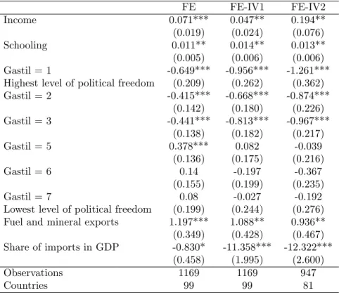
(33) F. Including Every Level of Political Freedom Income Schooling Gastil = 1 Highest level of political freedom Gastil = 2 Gastil = 3 Gastil = 5 Gastil = 6 Gastil = 7 Lowest level of political freedom Fuel and mineral exports Share of imports in GDP Observations Countries. FE 0.071*** (0.019) 0.011** (0.005) -0.649*** (0.209) -0.415*** (0.142) -0.441*** (0.138) 0.378*** (0.136) 0.14 (0.155) 0.08 (0.199) 1.197*** (0.349) -0.830* (0.458) 1169 99. FE-IV1 0.047** (0.024) 0.014** (0.006) -0.956*** (0.262) -0.668*** (0.180) -0.813*** (0.182) 0.082 (0.175) -0.197 (0.199) -0.027 (0.244) 1.088** (0.428) -11.358*** (1.995) 1169 99. FE-IV2 0.194** (0.076) 0.013** (0.006) -1.261*** (0.362) -0.874*** (0.226) -0.967*** (0.217) -0.039 (0.216) -0.367 (0.235) -0.192 (0.276) 0.936** (0.467) -12.322*** (2.600) 947 81. Standard errors in parenthesis (clustered std. errors in OLS, IV1, and IV2). ***,**,* indicate statistical signi…cance at the 1%, 5%, and 10% level respectively.. Table 10: All Political Freedom Dummies Included. 30.

(34)