Openness and Optimal Monetary Policy
Texte intégral
Figure
Documents relatifs
moreeconomic gains to the European consumers than the current EC proposal, and
Last but not least, the eurozone members are divided almost equally between the two groups of EU Member States (those with an improving export-import ratio, and the others) and, as a
This motivates our empirical strategy: we rst estimate sector- level trade elasticities, then compute price and income changes resulting from trade cost changes
The problem is that the WTO rules under the DSU do not allow collective retaliations, and the general principles of international law regarding collective measures embedded in
The importance of the exchange rate to monetary policy is reflected in large academic and policy-related literatures on the topic. We contribute to this literature by addressing
In this paper, we compare, …rst, the impact of a windfall and a boom sectors on the economy of an oil exporting country and their welfare implications; in a second step, we analyze
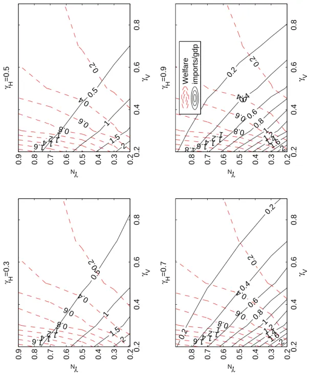
Elasticity of substitution between domestic and foreign goods () As stated above, the necessary condition for the real exchange rate to depreciate in response to an
If the intention of the central bank is to maximize actual output growth, then it has to be credibly committed to a strict inflation targeting rule, and to take the MOGIR
