Retirement age and senior workers’ employment: modelling the ‘distance-to-retirement’ effect

Retirement Age and Senior Workers’ Employment:

Modelling the ‘Distance-to-Retirement’ Effect

March 2012

Preliminary version. Do not quote.

Abstract

With the retirement reform of 2010, a new element has been taking into account in simulation model on retirement: the feedback effects on the labour market, or so-called ‘distance-to-retirement’ effect. The 2010 reform has increased the minimum legal age of retirement progressively from 60 to 62 years old, then, what people will do between these two ages (and before 60 if they change their behaviour)? Will they stay in employment? Will they be unemployed? This study analyses how to model the distance to retirement effect and the consequences of different assumptions on two projected indicators: the employment rate and the activity rate. If the assumptions made seem to entail similar activity rate, the employment rate can have a difference of 10 percentage points according to the assumption. The conclusion in terms of political economy can be radically different from ‘a better senior employment rate’ to ‘a larger unemployment rate’.

Key words: labour market, retirement behavior, microsimulation

Introduction

The French retirement reform of 2010 was intended to balance pension system by 2020. The main measure of this reform was to increase progressively (with a smoothing over 4 years) the minimum legal age of retirement, from 60 to 62 year old.

The efficiency of the reform is based on the capacity of the labour market to maintain older workers at work. Then, the modelling of the reform impact should take into account these consequences, especially in a microsimulation model on retirement.

During the last decades, most French workers have left (voluntary or not) the labour market during the last 5 years before the retirement legal age. In 2010, the employment rate dropped by 30 to 40 percentage points between 54 and 59 year old, i.e. one year before the minimum legal age (DARES, 2011).

The consequence for the modelling is that we should not only make assumptions on the impact of the reform on the labour market between 60 and 62 years old, but also few years before the minimum legal age.

The link between the senior employment rate and the minimum legal age of retirement is usually named ‘the distance to retirement effect’. It is defined by the impact of the retirement legislation on the labour market due to anticipation behaviour of workers and employers.

This link can also be due to the role of social institutions, such as unemployment insurance or disability benefits, which allow a specific status for elder workers close to retirement. Indeed, the increase in the minimum legal age for retirement might also increase the minimum legal age of several social arrangements (pre-retirement, disability or unemployment benefits…). This will be also the case for the private arrangements to guarantee that the enterprise’s pre-retirement program will not support a significant additional cost.

For the modelling, only the aggregate impact of all mechanisms (individual, institutional, employers…) is relevant, not the role played by each of them. So we intend to model the results of all of them taken together. Nevertheless, the ‘distance to retirement effect’ can be defined differently across studies, and then we discuss on the first part the definition of this concept.

The second part analyses how to take into account, in a simulation model on retirement, the impact of the increase of the retirement minimum legal age on the senior labour market. We illustrate this question using the PROMESS model developed by the DREES1 in 2010 (Aubert et al., 2010 et 2011). This model was created within the context of the retirement reform of 2010, then, the modelling of the impact of the increase of the minimum legal age was crucial to determinate the model structure. Indeed, the modelling was done in a way that makes it very easy to simulate and test several alternative assumptions concerning the elasticity of the older workers’ employment to the minimum legal age of retirement. The consequences on the labour market of these assumptions are presented in the third part. The quantitative analyse shows the uncertainty concerning the evolution of the labour market for seniors. It also permits to estimate the robustness of projected indicators such as senior employment rate or the labour market leaving age.

The ‘distance to retirement’: mechanisms and empirical proofs.

Theoretical arguments

The concept of ‘distance to retirement effect’ has gained increased attention in France since the studies on ‘distance effect’ of Hairault et al. (2006, 2010).

In their articles, the theoretical argument is based on the job return to investment, that is, the formation cost for the worker and for the employer. This return, as all returns, depends on the duration of the job. For elder workers, the two parts know that the horizon, (i.e. the depreciation period), is equal to the number of years before retirement, which is relatively short compared with younger employees. Their definition of the ‘distance effect’ includes several mechanisms which modify the supply and the demand of labour which itself depends on workers and unemployed old people.

Behaviour model on retirement define individual decision as a trade-off between cost and gain associated with different situations. Costs and gains are calculated both on present period and future periods. The future gains are positive only if people remain on the labour market, then they are weighted by the probability to stay on the labour market. These probabilities decrease rapidly to zero for people close to their retirement age. It’s by this way that theoretical model define the distance to retirement effect.

The concept of the ‘distance’ appears only when we want to simplify models for an empirical estimation. In this case, we use a proxy defined by the duration between two ages.

To apprehend this concept of distance to retirement effect, we should then define the reference age. Several ‘legal ages’ can be used for the French case: the minimum legal age for retirement, the legal age for a pension without financial penalties, the individual age for a pension without financial penalties… the theory can not help us because the real horizon is an anticipated age in expectancy. In Hairault et al. (2006), they opt for the minimum legal age for retirement for international comparisons but argue that for the empirical estimation is more relevant to take into account the individual age for a pension without financial penalties (which, in the French system, depends on the individual’s length of carreer). In a comment of this article, Blanchet (2006) wonders if it is relevant to take this individual age, indeed, workers and employers do not know this individual age but only the median or the modal social age.

This question is interesting because it determines the political decision. If the relevant age is the median or the modal social age, then a reform can have no effect on the labour market, even if the distance to retirement effect exists. The impact of this reform will appear only when the social median age will change, with no information about how long it will take.

Moreover the feedback effects on the labour market of the retirement legislation are not necessary due to the distance to retirement effect in this sense that they do not come from workers and employers behaviour. As mentioned previously, several institutional arrangements also have a minimum legal age. A modification of the minimum legal age for retirement may entail the same modification to benefit from these arrangements implying a modification of the labour market equilibrium. These consequences are not due to the distance to retirement effect2.

Another example illustrated by Aubert (2011), shows that people who already acquired the required insurance duration before the minimum legal age for retirement are more likely to leave the labour market a few years before the legal age. This can be due to private pre-retirement arrangements. Indeed, during this arrangement, individuals do not acquire insurance duration, then, a worker without this required insurance duration will not accept to leave the labour market for such arrangement.

Empirical Investigation

In Hairault et al. (2006), the stylised facts used to illustrate the distance to retirement effect come from both macro and micro economic estimations. At the macroeconomic level, they display the correlation between the minimum legal age for retirement and the relative senior-to-youngsters employment rate in several countries. They also use the historical evolution of the activity rate of the 55-59 years old people which decreased dramatically at the beginning of the 1980s’. They argue that this decrease is due to the retirement reform of 1983, which established the minimum legal age at 60 years old instead of 65 years old and then change the distance to retirement. In their study, they also estimate3 the probability to be in employment for every age since 50 years old according to individual characteristics (gender, degree, socio-professional category…), the age and the distance at the individual age for a pension without financial penalties (i.e. the age at which individual acquires the required insurance duration).

Their results show that the distance has a significant positive coefficient, i.e. the probability to be in employment is higher when the distance is greater. Then, the authors conclude that the distance to retirement effect exists.

These first results have entailed a debate on the interpretation of the econometric results (Benallah et

al., 2009 ; Hairault et al., 2009 et 2010 ; OFCE, 2009). The question focuses on the measure of the

distance until the retirement age. This age is estimated for every individual from its first employment

2 _{We could name it an ‘institutional effect’.}

age plus the required insurance duration. However, the first employment age can be correlated with individual characteristics no taken into account in the empirical estimation. Therefore, we can not interpret the significant coefficient. Particularly, it’s difficult to identify the effects of the ‘entry distance’ (i.e. the number of year since the first employment) and the effects of the ‘exit distance’ (i.e. the number of years until the retirement) when this last one is calculated using the first employment age. Using the same database, Benallah et al. (2009) estimate two regressions including the ‘entry distance’ for the first one and the ‘exit distance’ for the second. Results are statistically significant for both estimation but the interpretation can be radically different.

Nevertheless, both effects can be estimated jointly because the relation between the first employment age and the retirement age for a pension without financial penalties is not perfectly linear. Indeed, the retirement age is bounded on the right and the left: it can not be lesser than the minimum legal age (60 year old before the 2010 reform) and it can not be greater than the legal age for a pension without financial penalties (65 year old before the 2010 reform) whatever the first employment age is. This non-linear relation enables Hairault et al. (2009, 2010) to estimate simultaneously both effects. They confirm that an ‘entry distance’ exists and has an impact on the probability to be in employment but it is not a substitute to the ‘exit distance’. This last one is still statistically significant.

Another comments concerning these estimations was that their might be measurement errors. Indeed, the age of retirement without financial penalties is calculated using the first employment age plus the required insurance duration. Even if the sample only includes men working in the private sector, this is a bit frustrating because it does not take into account the inactivity period or unemployment without benefits… Using a more detailed database concerning individual pension rights (Pensioners’ Inter-scheme sample, DREES), Aubert (2011) confirms the existence of the ‘exit distance’ and the significant effect of a distance to retirement effect. Results show that a greater distance to retirement is associated with a lesser probability to leave the labour market for men between 57 and 59 years old.

Microeconometric results: qualitative rather than quantitative.

Available estimations conclude that a distance to retirement effect exists a few years before the retirement. This does not imply that this effect is the only one which determines the senior employment. Particularly, the age effects are also significant in all these estimations.

Moreover, econometric results do not directly provide estimation at the aggregate level of this effect. Thus, it is difficult to determine the aggregate impact of an increase of the minimum legal age of retirement on the labour market for elder workers.

The difference between the individual effect (the one of the econometric estimations) and the average effect on the population as a whole can have been the source of controversy in the public debate. Indeed, empirical studies results are made ceteris paribus, whereas the political reflection concerning the legal ages of retirement is made at the aggregate level.

A modelling for the senior workers labour market

The question in our study is how to quantify, in the context of a simulation model on retirement4, the overall impact on employment rates for senior workers of distance to retirement effects, or more generally the feedback impact of retirement reform on the labour market. To illustrate the sensitivity of different modelling of the distance to retirement effect, we use the PROMESS model (DREES).

First, it should be noted that for modelling the last decade of a professional career, we need to model two things: the labour market transitions (employment, inactivity, unemployment…) and the retirement decision, taking retirement legislation (minimum legal age, retirement age…) into account. These two events can be modelled jointly or separately. Nevertheless, the feedback effects of retirement legislation have an impact on the labour market transition, several years before the minimum legal age of retirement.

These feedback effects were taken into account since 2010 to estimate the impact of an increase of the minimum legal age of retirement. Note that this modelling can come from 2 channels (taken together or not):

- the individual channel for which the ‘distance to retirement ‘equals the distance to the age a to the individual age of retirement (which varies according to the individual’s lenght of carreer)5 - the social channel for which the distance to retirement effect depends on the minimum legal

age for retirement (the same for every people belonging to the same generation6)

The first channel is the real individual distance to retirement effect; the second can be viewed as a distance to retirement effect but in relation to a social norm and can also include the impact of other elements than the pure, stricly-speaking distance to retirement effec.

In practice, we choose to model the second channel (at least for the two models Destinie and Promess) because it is more global. The understanding of all the mechanisms is not essential for the functioning of the model7. We only should keep this choice in mind when interpreting the results.

Modelling issues

The distance to retirement effect modelling implies to modify the end of the professional career. The easiest way to model it is to postpone the age of leaving the labour market by the same proportion of the increase of the minimum legal age of retirement. For example, when the minimum legal age of retirement increases by one year, we postpone by one year all individual employment situations: all individuals in employment at 60 year old will be in employment at 61 year old, etc. We can also make the assumption that the proportion is lesser than 1 to take into account a partial feedback effect or for the transitional period before the total implementation of the reform. The proportionality coefficient is then ad-hoc. This type of assumption is made in Destinie for the 2010-2060 population projection exercise8.

An alternative modelling is made in the Promess model (for details see Aubert, et al., 2010 and 2011). This model was elaborated to prepare the retirement reform of 2010. The increase of the minimum legal age of retirement was explicitly announced among the options of the reform, so special attention to the distance to retirement effect has been made, particularly for the structure of our model. The

4

Several simulation models on retirement exist in France: DESTINIE by the Insee (National Statistic Institute), PRISME by CNAV (National pension organism), PROMESS by the DREES (Statistic Direction of the labour Ministry), VENUS by the Financial Directorate… DESTINIE is also used for the 2010-2060 active population projection which takes or not into account the horizon effect (Filatriau, 2011).

5 _{The French econometric studies used to refer to this channel because it’s the only age which has been modified} across time before the 2010 reform (due to the increase of the required insurance duration).

6 _{Except special cases such as earlier retirement for long career or specific categories of civil servant}

7 _{This choice is also easier to model. Nevertheless, there are no technical barriers to model the both channels in a} future version of our model.

8 _{The age of the labour market leaving is move forward according the individual retirement age (and not} according to the minimum legal age for retirement).

feedback effects are modelled postponing instantaneous probability associated to the labour market transitions.

For a minimum legal age for retirement at 60 year old, the age distributions for the labour market leaving age since 54 year old is modelled multiplying the instantaneous probability at 54 years, 55 years, etc, following equation (1)

employment employment employment employment employment

P

P

P

P

P

old

years

after

validation

old

years

at

employment

in

be

to

P

60 59 55 54 53

*

*

*

...

*

*

)

50

60

(

=

(1)

We define two ages (we have then two age distributions): an age for the employment leaving and an age for the labour market leaving (employment, unemployment, pre-retirement, and disability…, eg. each arrangements or situations which permit individuals to acquire insurance duration).

These probabilities are estimated separately for every age, for men and for women, according to the wage quartile between 50 and 54 years old, and according to the validation (or not) of the required insurance duration.

In projection, for simulations with an increase of the minimum legal age for retirement, we assume that the instantaneous probabilities of the 5 years before the minimum legal age are the same as the probabilities between 55 and 60 years old and every years before the last 5 years are similar to the probabilities at 54 year old9. For example:

(

employment employment employment

)

employment employment employment employment

P

P

P

P

P

P

P

old

years

after

validation

old

years

at

employment

in

be

to

P

60 59 55 54 54 54 53

*

*

*

*

*

...

*

*

)

50

62

(

=

(2)

This modelling consists in maintaining a constant distance to the minimum legal age for retirement, as far as probability of remaining in (or leaving) employment are concerned. Indeed, the instantaneous probability of permanent exit from employment at 59 year old becomes, ceteris paribus, the instantaneous probability of permanent exit from employment at 61 years old when the minimum legal age for retirement increases from 60 to 62 year old. This modification is not absolute concerning the probability to be in employment at the age a, because the postponement of the instantaneous probability does not imply the same postponement of the employment rate. For this last one, the evolution is lesser due to the application, as many times as there are years, of the instantaneous probability at 54 years old:

P

₅₄employment

Moreover, the postponement is not absolute also because it is ceteris paribus, and individual characteristics evolve across time (and age), and particularly concerning the insurance duration, one of the principal determinants of the employment.

Implicit assumptions

The offset of the instantaneous probabilities implies assumption on the feedback effects on the labour market. We present the interpretation we made of each of them. The figure 1 permits to apprehend the mechanisms.

Fact1: for each gender and wage quartile, the probability to stay in employment when individuals have not yet acquired the required insurance duration is high until 54 years old and decreases dramatically after this age (black curve) 10;

Fact2: people with sufficient required insurance duration have a lower probability to remain in employment particularly at 58 and 59 year old;

9 _{This modelling concerned people in employment at 50 years old. The probability} employment

P

53 is defined as the probability to be in employment at 53 years old knowing that individual was in employment at 50 years old. 10 _{Note that the probability at 60 years old is not comparable with the other ages in that sense that it represents} the probability to exit the labour market before the minimum legal age.

Fact3: the probability to remain ‘close to’ the labour market (including employment, unemployment, pre-retirement, disability, illness…) is close to one for people without a sufficient insurance duration;

Fact4: the probability to remain ‘close to” the labour market decreases after 57 year old for people with the required insurance duration

Figure 1

Probabilities to remain in employment and probability to remain close to the labour market, by age

Men 0,70 0,75 0,80 0,85 0,90 0,95 1,00 5 0 -5 3 (-6 ) 5 4 (-5 ) 5 5 (-4 ) 5 6 (-3 ) 5 7 (-2 ) 5 8 (-1 ) 5 9 (-0 ) 6 0 5 0 -5 3 (-6 ) 5 4 (-5 ) 5 5 (-4 ) 5 6 (-3 ) 5 7 (-2 ) 5 8 (-1 ) 5 9 (-0 ) 6 0 5 0 -5 3 (-6 ) 5 4 (-5 ) 5 5 (-4 ) 5 6 (-3 ) 5 7 (-2 ) 5 8 (-1 ) 5 9 (-0 ) 6 0 5 0 -5 3 (-6 ) 5 4 (-5 ) 5 5 (-4 ) 5 6 (-3 ) 5 7 (-2 ) 5 8 (-1 ) 5 9 (-0 ) 6 0

First (low er) w age quartile Second w age quartile Third w age quartile Fourth (upper) w age quartile age dis tance to retirem ent P ro b a b il it y t o s ta y e m p lo y e d ( re s p . c o n ti n u e v a li d a ti n g q u a rt e rs )

Stay at work: individuals without sufficient career duration Stay at work: individuals with sufficient career duration

Continue validating quarters: individuals without s ufficient career duration Continue validating quarters: individuals with sufficient career duration

Women 0,70 0,75 0,80 0,85 0,90 0,95 1,00 5 0 -5 3 (-6 ) 5 4 (-5 ) 5 5 (-4 ) 5 6 (-3 ) 5 7 (-2 ) 5 8 (-1 ) 5 9 (-0 ) 6 0 5 0 -5 3 (-6 ) 5 4 (-5 ) 5 5 (-4 ) 5 6 (-3 ) 5 7 (-2 ) 5 8 (-1 ) 5 9 (-0 ) 6 0 5 0 -5 3 (-6 ) 5 4 (-5 ) 5 5 (-4 ) 5 6 (-3 ) 5 7 (-2 ) 5 8 (-1 ) 5 9 (-0 ) 6 0 5 0 -5 3 (-6 ) 5 4 (-5 ) 5 5 (-4 ) 5 6 (-3 ) 5 7 (-2 ) 5 8 (-1 ) 5 9 (-0 ) 6 0

First (low er) w age quartile Second w age quartile Third w age quartile Fourth (upper) w age quartile age dis tance to retirem ent P ro b a b il it y t o s ta y e m p lo y e d ( re s p . c o n ti n u e v a li d a ti n g q u a rt e rs )

Stay at work: individuals without s ufficient career duration Stay at work: individuals with sufficient career duration

Continue validating quarters: individuals without sufficient career duration Continue validating quarters: individuals with sufficient career duration

Note 1: men belonging to the first quartile of wage, with the required insurance duration and who are on the labour market at 59 years old have a probability of 0.95 to be on the labour market at 60 years old

Note 2: indivudals who finish their professional career in the private salary sector. Sources: Drees, Promess, EIC 2005 (Contributors’ Inter-scheme sample)

Facts2 2 and 4 can be a consequence of arrangements which not permit to acquire insurance duration (firm-funded pre-retirement schemes or the so-called ARPE public pre-retirement scheme). Such

arrangements are of course subscribed only by individuals who have a sufficient insurance duration because they are the only one not to be penalised by these arrangements in terms of pension rights. We can then assume that the differential of probabilities between people with sufficient insurance duration and people without it is a proxy of the proportion of people leaving the labour market to enter such arrangements. As the probabilities differ particularly between 57 and 59 years old, to neutralize the effect of such arrangements for a modeling, we need to remove the probabilities differences. An alternative method will consist in replacing the instantaneous probability at 57-58 and 59 years old by the instantaneous probability observed at 56 years old.

For the PROMESS model, we assume that these arrangements will be still relevant in the future and in the same proportion11. The only difference is that the cost for employers or social institutions will be the same, then, the minimum age of theses arrangements will be delayed.

Fact 3 is due to the fact that generally, after employment, people enter a period of unemployment, illness or disability which permits to acquire insurance duration until their retirement age without financial penalties.

Fact 1 has three interpretations. First, the distance to retirement effect has a role only during the five years before the minimum legal age of retirement; second, the instantaneous probability at 54 year old is a good proxy of the instantaneous probability without a distance to retirement effect (that is, only due to the age effects); third, the difference between the instantaneous probability at 54 year old and the instantaneous probability after this age can be due to the distance to retirement effect. Indeed, if the determinants of the seniors’ employment are only due to their productivity or capacities, the probabilities should be decreasing with age and not drop dramatically at 55 years old.

These three elements entail us to assume for the PROMESS model that when the minimum legal age of retirement increases from 60 to 62 years old, the instantaneous probabilities at 55 and 56 years old are the instantaneous probability observed at 54 years old before the reform.

These interpretations are only used to explain the different assumptions retained for the PROMESS model and the choice concerning the alternative simulations.

Variation in assumptions

Table 1 presents the different assumptions we make for the modelling of the feedback effects of the 2010 retirement reform on the labour market. These assumptions are applied only on individuals who finish their professional career in the private sector12. Each of them makes an implicit assumption on the labour market.

- The ‘total move’ assumption (HTC): this assumption supposes that the seniors remain on employment with certainty at 54 and 55 years old. After 55 years old, probabilities observed the last 5 years before the new minimum legal age of retirement are similar to the probabilities observed between 55 and 60 year old before the reform. This is a strong assumption because it supposes that there is no employment exit between 53 and 55 year old and that all arrangements (as private pre-retirement) still exist and their access (in terms of age) is modified as the minimum legal age of retirement.

- The ‘high move’ assumption (54a) is the assumption used for the preparation of the retirement reform of 2010. It is similar to the HTC assumption, except that the instantaneous probabilities to leave employment and to leave the labour market at 55 and 56 year old are the same as the instantaneous probabilities at 54 years old before the reform.

- The ‘pre-retirement removal’ assumption (HH) is the 54a assumption until 58 years old. From 59 to 61 year old, the instantaneous probabilities are the ones of the 56 years old before the reform, that is, no more pre-retirement arrangements from 59 years old. This assumption will entail a greater employment rate compared with the 54a assumption.

11 _{We do not assume that in the future the same arrangements will exist (we already know that the employment} replacement allocation does not exist anymore) but that the same kind of arrangements will persist, with the same consequences on the labour market.

12

For workers finishing their professional career in the public or special sector, the labour market exit is due to the retirement. For these categories, the retirement takes place as soon as individuals validate the insurance duration.

- The ‘median’ assumption (56a) makes no modification until 56 year old. After this age, at 57 and 58 years old, the instantaneous probabilities are similar to the ones of the 56 years old before the reform. As the employment rate is lower at 56 years than at 54 years old, we can expected a lower employment rate for this simulation compared with the 54a simulation. - The ‘low’ assumption (58a) keeps the same probabilities until 58 years old. At 59 and 60 years

old, the instantaneous probabilities are the ones of the 58 year old before the reform. The expected employment rate is then lower compared with the 54a and 56a assumptions. Moreover, the ‘low’ assumption considers that the age condition for all pre-retirement arrangements is unchanged; therefore, the duration of these arrangements will be longer. - The last three assumptions keep the same probabilities until 60 years old before and after the

reform. The ‘stability after 60 years old’ assumption (EMP_60) assumes that individuals still in employment at this age will remain on the labour market until the minimum legal age of retirement. The ‘60a’ assumption applies the 60 years old instantaneous probabilities at 61 and 62 years old. Finally, the ‘median alternative’ assumption (56b) duplicates the instantaneous probabilities of 56 years old before the reform at 61 and 62 years old. As the employment rate at 60 years old before the reform is low, we can expect a lower employment rate for these 3 simulations compared with the others.

Table 1

Probability of remaining in employment at each age, under several assumptions of the feedback effects

Age

Before 2010

After 2010

(minimum legal age of retirement at 62 years old)

Assumption =

‘total move’ assumption ‘pre-retirement removal’ ‘high move’ assumption (Promess) ‘median’ assumption ‘low’ assumption ‘60a’ assumption ‘median alternative’ assumption ‘stability after 60 years old’ assumption

HTC

HH

54A

56A

58A

60A

56B

emp_60

54

P

54

1

P

54

P

54

P

54

P

54

P

54

P

54

P

54

55

P

55

1

P

54

P

54

P

55

P

55

P

55

P

55

P

55

56

P

56

P

54

P

54

P

54

P

56

P

56

P

56

P

56

P

56

57

P

57

P

55

P

55

P

55

P

56

P

57

P

57

P

57

P

57

58

P

58

P

56

P

56

P

56

P

56

P

58

P

58

P

58

P

58

59

P

59

P

57

P

56

P

57

P

57

P

58

P

59

P

59

P

59

60

P

60

P

58

P

56

P

58

P

58

P

58

P

60

P

60

P

60

61

P

59

P

56

P

59

P

59

P

59

P

60

P

56

1

62

P

60

P

60

P

60

P

60

P

60

P

60

P

56

1

Note: the probabilities Pa are estimated at the age a on the observed data before the reform of 2010

on the generation born in 1934, 1938 and 1942.

Graph 2 represents three of these assumptions for men born in 1970 and belonging to the second quartile of wage. The area below the curves in Graph 3 permits to compare the impact of simulation assumptions on employment rates at each age.

The ‘low’ assumption implies, as expected, a lower employment rate compared with the ‘total’ assumption.

The expected employment rate for people who validated the required insurance duration should be lower at the minimum legal age for retirement compared with people who did not validate it. In practice, the insurance duration increases with the age in our model, therefore, people who did not validate the insurance duration at 54 years old can jump in the other group before the minimum legal age for retirement.

Graph 2. Instantaneous probabilities to remain in employment, by quarterly age Men belonging to the second quartile of wage, born in 1970

96,5% 97,0% 97,5% 98,0% 98,5% 99,0% 99,5% 100,0% 5 4 5 5 5 6 5 7 5 8 5 9 6 0 6 1 6 2 5 4 5 5 5 6 5 7 5 8 5 9 6 0 6 1 6 2

Age (without sufficient insurance duration) Age (with sufficient insurance duration)

Simulation

Total (HTC) Promess (54a) Low (58a) Sources: Drees, Promess

Note1: men who finish their professional career in the private sector, belonging to the second quartile of wage and born in 1970.

Note2: Under the ‘total’ assumption, men have a probability to remain in employment at 54 years old equals to 1 whatever their insurance duration.

Remark: the probabilities are not comparable with the graph 1 because the age is annual for the graph 1 and quarterly in this graph.

Graph 3. Cumulated probabilities to stay in employment after age 50, by quarterly age Population born in 1970 0,0% 10,0% 20,0% 30,0% 40,0% 50,0% 60,0% 70,0% 80,0% 90,0% 100,0% 54 55 56 57 58 59 60 61 62 63 64 65 66 67 68 Simulation

Total (HTC) Promess (54a) Low (58a)

Note: people who finish their professional career in the private sector. Sources: Drees, Promess

Simulation sensitivity according to the assumptions

We analyse the impact of these different assumptions according to several points of view. We first pay attention to the activity rate for the 55-59 year old in projection and second, to the projected employment rate. ‘Activity rate’ is here defined as the share of people in employment or in any arrangement that implies acquiring insurance duration within the population. It is therefore distinct to the more usual ILO activity rate.

With the retirement reform of 2010, we can expect that the age of leaving the labour market will increase and then entail an increase of the validated insurance duration for elder workers. At the same time, the legal required insurance duration increases over generations. To distinguish each of them, we simulate several scenarii taking into account (separately or simultaneously) the increase of the insurance duration and the increase of the minimum legal age of retirement.

1. Activity rate projections from 2010 to 2030

For men, the differences between the assumptions for the modeling of the feedbacks effects are not really relevant (graph 4); the activity rate has no more than 2 percentage points of differences whatever the simulation is.

However, for women, even if the modeling assumptions have no differences greater than 3 points of per cent, a modeling is necessary, the simulation ‘before the 2010 reform being statistically lower than the others.

Graph 4. Activity rate (employment or assimilated period) of 55-59 years old for the private sector

65% 70% 75% 80% 85% 2 0 1 0 2 0 1 5 2 0 2 0 2 0 2 5 2 0 3 0 2 0 1 0 2 0 1 5 2 0 2 0 2 0 2 5 2 0 3 0 Men Women

Before the 2010 reform Promess (54a)

Median (56a) Low (58a)

Preretirement removal (HH) Total (HTC) Note1: people who finish their professional career in the private sector. Sources: Drees, Promess

2. Employment rate projections from 2010 to 2030

The projected employment rates for the 55-59 year old rise sharply for the stronger assumptions (graph 5 and 6): plus 6 percentage points for the 54a assumption and plus 9-10 points for the HTC simulation compared with a scenario without an increase of the minimum legal age of retirement (before the 2010 reform).

The median assumption (56a) is a quite upper to the other ‘soft’ simulations (1 point for men and 0.5 point for women).

At least, the low (58a) assumption seems to have no effect on the labour market for men (compared with the simulation without reform), contrary to women. These results can be explained by other mechanisms such as the removal of the possibility to retire earlier for the 3 children mothers in the public sector.

The first lesson on these results is that the assumption made in terms of distance to retirement effect, that is, the feedback effects on the labour market of the retirement legislation, is not without consequences for the political decision. If the modeling chosen is one of the strongest assumptions, then one can conclude that an increase of the minimum legal age of retirement can entail a better employment rate for older workers. On the contrary, if the modeling chosen is one of the lowest assumptions, then the conclusion will be that an increase of the minimum legal age of retirement will entail unemployment.

Graph 5. Employment rate of 55-59 year old

45% 50% 55% 60% 65% 70% 75% 2 0 1 0 2 0 1 5 2 0 2 0 2 0 2 5 2 0 3 0 2 0 1 0 2 0 1 5 2 0 2 0 2 0 2 5 2 0 3 0 Men Women

Before the 2010 reform Promess (54a)

Median (56a) Low (58a)

Preretirement removal (HH) Total (HTC) Note: all the population.

Graph 6. Sliding employment rate the last five years before the minimum legal age (55-59 year old and progressively 57-61 year old)

40% 45% 50% 55% 60% 65% 2 0 1 0 2 0 1 5 2 0 2 0 2 0 2 5 2 0 3 0 2 0 1 0 2 0 1 5 2 0 2 0 2 0 2 5 2 0 3 0 Men Women

Promess (54a) Median (56a)

Low (58a) 60a

Preretirement removal (HH) Total (HTC) Note1: people who finish their professional career in the private sector.

Note2: the employment rate is calculated every year as the number of people in employment over all the population for the generations aged to [minimum legal age – 5; minim legal age [.

Sources: Drees, Promess

3.

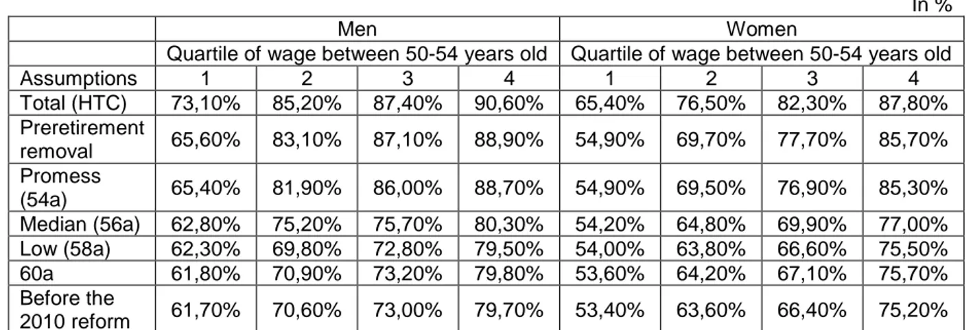
Intermediate wage quartile more affected by the assumptions

The assumptions have a relatively low effect for individuals within the first quartile of wage,

except for the ‘total’ one which entails an increase of the employment rate of more than 10

points (table 2).

For the three ‘high’ assumptions (HTC, HH and 54a) the employment rate is greater for the

second and the third quartile of wage about 13 percentage points for men and 6 to 16

percentage points for women.

For men, these results can be explained by the fact that the intermediate quartiles of wage are

composed by individuals who can ‘choose’ their employment status. Indeed, in these

quartiles, people have a relatively long insurance duration and they can enter private or public

arrangements before the retirement. Assumptions which remove or delay this kind of

arrangements are then more important for them.

On the contrary, in the first quartile of wage as in the upper one, people have not enough

insurance duration. For the first quartile of wage this is due to a lesser safety implementation

of the labor market, particularly because of part-time work or mini-jobs which do not permit

to acquire 4 quarters by year. For the upper quartile, the story is different: it concerns people

who enter the labor market relatively later because of a higher education. For them, the

insurance duration criterion is not satisfied before the minimum legal. So if this minimum

legal increases they should and could stay in employment until the new age of retirement

whatever the assumption is.

Overall, the assumptions have a slightly lesser impact on the employment rate of women than

of men. For the first two quartiles of wage, this can be explained by the fact that women

usually don’t have a sufficient insurance duration and then wait for the age which permits a

pension without financial penalties (the maximum legal age). So, whatever the assumption is,

they do not have more or less incitation to stay or leave the labor market.

Table 2. 55-59 year old employment rate in 2020

In %

Men Women

Quartile of wage between 50-54 years old Quartile of wage between 50-54 years old

Assumptions 1 2 3 4 1 2 3 4 Total (HTC) 73,10% 85,20% 87,40% 90,60% 65,40% 76,50% 82,30% 87,80% Preretirement removal 65,60% 83,10% 87,10% 88,90% 54,90% 69,70% 77,70% 85,70% Promess (54a) 65,40% 81,90% 86,00% 88,70% 54,90% 69,50% 76,90% 85,30% Median (56a) 62,80% 75,20% 75,70% 80,30% 54,20% 64,80% 69,90% 77,00% Low (58a) 62,30% 69,80% 72,80% 79,50% 54,00% 63,80% 66,60% 75,50% 60a 61,80% 70,90% 73,20% 79,80% 53,60% 64,20% 67,10% 75,70% Before the 2010 reform 61,70% 70,60% 73,00% 79,70% 53,40% 63,60% 66,40% 75,20%

Conclusion

The modification of the minimum legal age for retirement has an impact on individual behaviour towards the labour market. This ‘distance to retirement’ is now known and shown thanks to the econometric analyses. However, these econometrical estimations do not quantify the effect and the simulation models are then helpful to provide relevant information to policy makers.

We use the PROMESS model which was developed for the 2010 retirement reform. This model pays a particular attention to the modelling of the feedback effects of the retirement legislation on the labour market. However, it takes into account all the mechanisms together (workers and employers behaviours, institutional arrangements, private preretirement grants…), without separately quantifying the effect of each of them.

Nevertheless, we show in this paper that the assumption made in terms of ‘distance to retirement’ modelling is not neutral for the political decision. Indeed, the employment rate of senior workers can be similar before and after the reform or can increase by 10 percentage points according to the assumption made.

Bibliography

AUBERT P. (2011), « L'effet horizon : de quoi parle-t-on ? », document n°6 de la séance plénière du Conseil d'orientation des retraites du 4 mai 2011

AUBERT P. (2011), « Effets directs et indirects des systèmes de retraite sur l'emploi des seniors : résultats récents », forthcoming in Revue française des affaires sociales

AUBERT P.,C.DUC ET B.DUCOUDRE (2010), « Le modèle Promess : projection "méso" des âges de cessation d'emploi et de départ à la retraite », Document de travail de la Drees - série Études et Recherches, n°102, décembre

AUBERT P.,C.DUC ET B.DUCOUDRE (2011), « Projeter l’impact des réformes des retraites sur les sorties d’activité : Une illustration par le modèle PROMESS », forthcoming in Revue française des

affaires sociales

BACHELET M., M. BEFFY ET D. BLANCHET (2011), « Projeter l’impact des réformes des retraites sur l’activité des 55 ans et plus : une comparaison de trois modèles », Document de travail de l’Insee, G2011/08

BENALLAH S.,DUC C.,LEGENDRE F. (2008), « Peut-on expliquer le faible taux d’emploi des seniors en France ? », Revue de l’OFCE, n°105, pp. 5-17

BLANCHET D. (2006), « Age ou distance à la retraite : quel est le principal déterminant de l’emploi des seniors ? », Économie et Statistique, n°397, pp. 65-68

DARES (2011), « L’emploi des seniors », présentation au Conseil national de l’information statistique (CNIS) du 4 avril 2011

FILATRIAU O. (2011), « Projections à l’horizon 2060 : des actifs de plus en plus nombreux », Insee

Première, n°1345 (avril)

HAIRAULT J.-O.,LANGOT F.,SOPRASEUTH T. (2006), « Les effets à rebours de l’âge de la retraite sur le taux d’emploi des seniors », Économie et Statistique n°397

HAIRAULT J.-O.,LANGOT F.,SOPRASEUTH T. (2009), « Le faible taux d’emploi des seniors : distance à l’entrée dans la vie active ou distance à la retraite ? », Revue de l’OFCE, n°109, pp. 63-84

HAIRAULT J.-O., LANGOT F., SOPRASEUTH T. (2010), “Distance to Retirement and Older Workers' Employment: The Case For Delaying The Retirement Age”, Journal of the European Economic

Association, vol 8 (5), pp. 1034-1076.

OFCE (2009), « Comment allonger les carrières ? Faut-il repousser l’âge légal de la retraite ? Rencontre d’experts organisés par l’OFCE le 10 mars 2009 », Revue de l’OFCE, n° 109, pp. 85-99