Generalized Mahler measure of a family of polynomials
Texte intégral
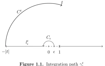
Figure


Documents relatifs
Based on deep results of Bourgain-Gamburg (2007) on expanders from SL(2,
Lehmer conjecture, Lehmer problem, Lehmer’s number, Schinzel-Zassenhaus conjecture, mapping class, stretch factor, coxeter system, Salem number, Perron number, Pisot number,
Theorem 1.3 generalizes to a lower bound for the normalized height of a hypersurface defined and irreducible over a number field (theorem 3.4 and remark 3.6)... I would like to
In our proof of theorem 2, we use a classical criterion of algebraic in- dependence of Loxton and van der Poorten; this criterion is used in many articles about the
A more classical way to construct a generator for the Galois closure of Q (β) is given by the proof of the Primitive Element Theorem, thus taking a general linear combination of
In this article we develop a new method for relating Mahler measures of three- variable polynomials that define elliptic modular surfaces to L-values of modular forms.. Using an idea
Corollary 1.1 applied with the functions 1, f (z) shows the contribution of Theorem 1.2 in understanding the nature of f (α) when α is regular. Corollary 1.2 below states that
L’archive ouverte pluridisciplinaire HAL, est destinée au dépôt et à la diffusion de documents scientifiques de niveau recherche, publiés ou non, émanant des
