HAL Id: hal-00785598
https://hal.archives-ouvertes.fr/hal-00785598
Submitted on 6 Feb 2013
HAL is a multi-disciplinary open access
archive for the deposit and dissemination of
sci-entific research documents, whether they are
pub-lished or not. The documents may come from
teaching and research institutions in France or
abroad, or from public or private research centers.
L’archive ouverte pluridisciplinaire HAL, est
destinée au dépôt et à la diffusion de documents
scientifiques de niveau recherche, publiés ou non,
émanant des établissements d’enseignement et de
recherche français ou étrangers, des laboratoires
publics ou privés.
Octagonal Domains for Continuous Constraints
Marie Pelleau, Charlotte Truchet, Frédéric Benhamou
To cite this version:
Marie Pelleau, Charlotte Truchet, Frédéric Benhamou. Octagonal Domains for Continuous
Con-straints.
17th International Conference on Principles and Practice of Constraint Programming
(CP’11), 2011, Perrugia, Italy. pp.706–720. �hal-00785598�
Octagonal Domains for Continuous Constraints
Marie Pelleau, Charlotte Truchet, Fr´ed´eric Benhamou
LINA, UMR CNRS 6241 Universit´e de Nantes, France [email protected]
Abstract. Domains in Continuous Constraint Programming (CP) are generally represented with intervals whose n-ary Cartesian product (box) approximates the solution space. This paper proposes a new representa-tion for continuous variable domains based on octagons. We generalize local consistency and split to this octagon representation, and we propose an octagonal-based branch and prune algorithm. Preliminary experimen-tal results show promising performance improvements on several classical benchmarks.
1
Introduction
Continuous Constraint Programming (CP) relies on interval representation of the variables domains. Filtering and solution set approximations are based on Cartesian products of intervals, called boxes. In this paper, we propose to im-prove the Cartesian representation precision by introducing an n-ary octagonal representation of domains in order to improve filtering accuracy.
By introducing non-Cartesian representations for domains, we do not mod-ify the basic principles of constraint solving. The main idea remains to reduce domains by applying constraint propagators that locally approximate constraint and domains intersections (filtering), by computing fixpoints of these operators (propagation) and by splitting the domains to search the solution space. Never-theless, each of these steps has to be redesigned in depth to take the new domains into account, since we lose the convenient correspondence between approximate intersections and domain projections.
While shifting from a Cartesian to a relational approach, the resolution pro-cess is very similar. In the interval case, one starts with the Cartesian product of the initial domains and propagators reduce this global box until reaching a fixpoint. In the octagonal case, the Cartesian product of the initial domains is itself an octagon and each constraint propagator computes in turn the smallest octagon containing the intersection of the global octagon and the constraint it-self, until reaching an octagonal fixpoint. In both cases, splitting operators drive the search space exploration, alternating with global domain reduction.
The octagon are chosen for different reasons: they represent a reasonable tradeoff between boxes and more complex approximation shapes (e.g. polyhe-dron, ellipsoids) and they have been studied in another context to approximate numerical computations in static analysis of programs. More importantly, we
show that octagons allows us to translate the corresponding constraint systems in order to incorporate classical continuous constraint tools in the resolution.
The contributions of this paper concern the different aspects of octagon-based solving. First, we show how to transform the initial constraint problem to take the octagonal domains into account. The main idea here is to combine classical constraint matrix representations and rotated boxes, which are boxes defined in different π/4 rotated bases. Second, we define a specific local consis-tency, oct-consisconsis-tency, and propose an appropriate algorithm, built on top of any continuous filtering method. Third, we propose a split algorithm and a notion of precision adapted to the octagonal case.
After some preliminary notions on continuous CSPs and octagons (Section 2), we present in Section 3 the octagon representation and the notion of octagonal CSP. Section 4 addresses octagonal consistency and propagation. The general solver, including discussions on split and precision is presented in Section 5. Finally, experimental results are presented in Section 6, related work in Section 7, while conclusion and future work end the presentation of this work.
2
Preliminaries
This section recalls basic notions of CP and gives material on octagons from [9]. 2.1 Notations and Definitions
We consider a Constraint Satisfaction Problem (CSP) on variables V = (v1...vn),
taking their values in domains D = (D1...Dn), with constraints (C1...Cp). The
set of tuples representing the possible assignments for the variables is D = D1×
...×Dn. The solutions of the CSP are the elements of D satisfying the constraints.
We denote by S the set of solutions, S = {(s1...sn) ∈ D, ∀i ∈ 1..n, Ci(s1...sn)}.
In the CP framework, variables can either be discrete or continuous. In this article, we focus on real variables. Domains are subintervals of R whose bounds are floating points, according to the norm IEEE 754. Let F be the set of floating points. For a, b ∈ F, we can define [a, b] = {x ∈ R, a ≤ x ≤ b} the real interval delimited by a and b, and I = {[a, b], a, b ∈ F} the set of all such intervals. Given an interval I ∈ I, we write I (resp. I) its lower (resp. upper) bound, and, for any real point x, x its floating-point lower approximation (resp. x, upper). A cartesian product of intervals is called a box. For CSPs with domains in I, constraint solver usually return a box containing the solutions, that is, an overapproximation for S.
The notion of local consistency is central in CP. We recall here the defini-tion of Hull-consistency, one of the most usual local consistency for continuous constraints.
Definition 1 (Hull-Consistency). Let v1...vn be variables over continuous
domains represented by intervals D1...Dn∈ I, and C a constraint. The domains
D1...Dn are said Hull-consistent for C iff D1× ... × Dn is the smallest
Given a constraint C over domains D1...Dn, an algorithm that computes the
local consistent domains D′
1...D′n, such that ∀i ∈ 1...n, Di′ ⊂ Di and D1′...D′n
are locally consistent for C, is called a propagator for C. The domains which are locally consistent for all constraints are the largest common fixpoints of all the constraints propagators [2, 12]. Practically, propagators often compute overapproximations of the locally consistent domains. We will use the standard algorithm HC4 [3]. It efficiently propagates continuous constraints, relying on the syntax of the constraint and interval arithmetic [10]. It generally does not reach Hull consistency, in particular in case of multiple occurrences of the variables.
Local consistency computations can be seen as deductions, performed on domains by analyzing the constraints. If the propagators return the empty set, the domains are inconsistent and the problem has no solution. Otherwise, non-empty local consistent domains are computed. This is often not sufficient to accurately approximate the solution set. In that case choices are made on the variables values. For continuous constraints, a domain D is chosen and split into two (or more) parts, which are in turn narrowed by the propagators. The solver recursively alternates propagations and splits until a given precision is reached. In the end, the collection of returned boxes covers S, under some hypotheses on the propagators and splits [2].
2.2 Octagons
In geometry, an octagon is a polygon having eight faces in R2 1. In this paper,
we use a more general definition given in [9].
Definition 2 (Octagonal constraints). Let vi, vj be two real variables. An
octagonal constraint is a constraint of the form ±v1± v2≤ c with c ∈ R.
For instance in R2, octagonal constraints define straight lines which are par-allel to the axis if i = j, and diagonal if i 6= j. This remains true in Rn, where
the octagonal constraints define hyperplanes.
Definition 3 (Octagon). Given a set of octagonal constraints O, the subset of Rn points satisfying all the constraints in O is called an octagon.
Remark 1. Here follows some general remarks on octagons :
– The geometric shape defined above includes the geometric octagons, but also other polygons (e.g. in R2, an octagon can have less than eight faces);
– an octagon can be defined with redundant constraints (for example v1−v2≤
c and v1− v2≤ c′), but only one of them defines a face of the octagon (the
one with the lowest constant in this example),
– in Rn, an octagon has at most 2n2 faces, which is the maximum number of
possible non-redundant octagonal constraints on n variables,
– an octagon is a set of real points, but, like the intervals, they can be restricted to have floating-points bounds (c ∈ F).
In the following, octagons are restricted to floating-point octagons. Without loss of generality, we assume octagons to be defined with no redundancies.
2.3 Matrix Representation of Octagons
An octagon can be represented with a difference bound matrix (DBM) as de-scribed in [8, 9]. This representation is based on a normalization of the octagonal constraints as follows.
Definition 4 (difference constraints). Let w, w′ be two variables. A
differ-ence constraint is a constraint of the form w − w′≤ c for c a constant.
By introducing new variables, it is possible to rewrite an octagonal constraint as an equivalent difference constraint: let C ≡ (±vi ± vj ≤ c) an octagonal
constraint. Define the new variables w2i−1 = vi, w2i = −vi, w2j−1 = vj, w2j =
−vj. Then
– for i 6= j
• if C ≡ (vi− vj ≤ c), then C is equivalent to the difference constraints
(w2i−1− w2j−1≤ c) and (w2j− w2i≤ c),
• if C ≡ (vi+ vj ≤ c), then C is equivalent to the difference constraints
(w2i−1− w2j≤ c) and (w2j−1− w2i≤ c),
• the two other cases are similar, – for i = j
• if C ≡ (vi− vi≤ c), then C is pointless, and can be removed,
• if C ≡ (vi+ vi) ≤ c), then C is equivalent to the difference constraint
(w2i−1− w2i≤ c),
• the two other cases are similar.
In what follows, regular variables are always written (v1...vn) , and the
cor-responding new variables are written (w1, w2, ...w2n) with: w2i−1 = vi, and
w2i = −vi. As shown in [9], the rewritten difference constraints represent the
same octagon as the original set of octagonal constraints, by replacing the posi-tive and negaposi-tive occurrences of the vivariables by their wicounterparts. Storing
difference constraints is thus a suitable representation for octagons.
Definition 5 (DBM). Let O be an octagon in Rn, and its sequence of potential
constraints as defined above. The octagon DBM is a 2n × 2n square matrix, such that the element at row i, column j is the constant c of the potential constraint wj− wi≤ c.
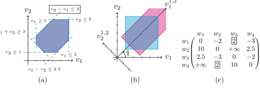
An example is shown on Figure 1(c): the element on row 1 and column 3 corresponds to the constraint v2− v1≤ 2 for instance.
At this stage, different DBMs can represent the same octagon. For example on Figure 1(c), the element row 2 and column 3 can be replaced with 100, for instance, without changing the corresponding octagon. In [9], an algorithm is defined so as to optimally compute the smallest values for the elements of the DBM. This algorithm is adapted from the Floyd-Warshall shortest path algorithm [6], modified in order to take advantage of the DBM structure. It exploits the fact that w2i−1 and w2i correspond to the same variable. It is fully
3
Boxes Representation
In the following section we introduce a box representation for octagons. This representation, combined with the DBM will be used to define, from an initial set of continuous constraints, an equivalent system taking the octagonal domains into account.
3.1 Intersection of boxes
In two dimensions, an octagon can be represented by the intersection of one box in the canonical basis for R2, and one box in the basis obtained from the
canonical basis by a rotation of angle π/4 (see figure 1(b)). We generalize this remark to n dimensions.
Definition 6 (Rotated basis). Let B = (u1, ..., un) be the canonical basis of
Rn. Let α = π/4. The (i,j)-rotated basis Bi,j
α is the basis obtained after a rotation
of α in the subplane defined by (ui, uj), the other vectors remaining unchanged:
Bi,j
α = (u1, ..., ui−1, (cos(α)ui+sin(α)uj), ...uj−1, (−sin(α)ui+cos(α)uj), ...un).
By convention, for any i ∈ {1...n}, Bi,i
α represents the canonical basis. In
what follows, α is always π/4 and will be omitted. Finally, every variable v living in the Bi,j rotated basis and whose domain is D will be denoted by vi,j
and its domain by Di,j).
The DBM can also be interpreted as the representation of the intersection of one box in the canonical basis and n(n − 1)/2 other boxes, each one living in a rotated basis. Let O be an octagon in Rn and its DBM M , with the same
notations as above (M is a 2n × 2n matrix). For i, j ∈ {1...n}, with i 6= j, let Bi,jO be the box I1× ... × Iii,j× ... × I
i,j
j ... × In, in Bi,j, such that ∀k ∈ {1...n}
Ik = −12M [2k − 1, 2k] Ik= 12M [2k, 2k − 1] Iii,j = − 1 √ 2M [2j − 1, 2i] I i,j i = 1 √ 2M [2j, 2i − 1] Iji,j = −√12M [2j − 1, 2i − 1] I i,j j = √12M [2j, 2i]
Proposition 1. Let O be an octagon in Rn, and Bi,j
O the boxes as defined above.
Then O = T
1≤i,j≤nB i,j O .
Proof. Let i, j ∈ {1..n}. We have vi,ji = 1/
√ 2(vi+ vj) and v i,j j = 1/ √ 2(vi− vj)
by definition 6. Thus (v1...vi,ji ...v i,j
j ...vn) ∈ B i,j
O iff it satisfies the octagonal
con-straints on vi and vj, and the unary constraints for the other coordinates, in
the DBM. The box Bi,jO is thus the solution set for these particular octagonal constraints. The points in T
1≤i,j≤nB i,j
O are exactly the points which satisfy all the
v1 v2 v1 ≥ 1 v1 ≤ 5 v2 ≥ 1 v2 ≤ 5 v2 − v1 ≤ 2 v1 − v2 ≤ 2.5 v1 + v2 ≥ 3 (a) v1,21 v21,2 v1 v2 π 4 (b) w4 w3 w2 w1 w4 w3 w2 w1 0 −2 2 −3 10 0 +∞ 2.5 2.5 −3 0 −2 +∞ 2 10 0 (c)
Fig. 1.Equivalent representations for the same octagon: the octagonal constraints 1(a), the intersection of boxes 1(b), and the DBM 1(c).
Example 1. Considering the DBM Figure 1(c), the boxes are I1× I2= [1, 5] ×
[1, 5], and I11,2× I 1,2 2 = [3/
√
2, +∞] × [−2.5/√2,√2].
To summarize, an octagon with its DBM representation can also be inter-preted as a set of octagonal constraints (definition in intension) or equivalently as an intersection of rotated boxes (definition in extension), at the cost of a mul-tiplication / division with the appropriate rounding mode. We show below that the octagonal constraints (or the bounds in the case of boxes) can be inferred from the CSP.
3.2 Octagonal CSP
Consider a CSP on variables (v1...vn) in Rn. The goal is now to equip this CSP
with an octagonal domain. We detail here how to build an octagonal CSP from a regular one, and show that the two systems are equivalent.
First, the CSP is associated to an octagon, by stating all the possible octag-onal constraints ±vi± vj ≤ ck for i, j ∈ {1...n}. The constants ck represent the
bounds of the octagon boxes and are dynamically modified. They are initialized to +∞.
The rotations defined in the previous section introduce new axes, that is, new variables vi,ji . Because these variables are redundant with the regular ones,
they are also linked through the CSP constraints (C1...Cp), and these constraints
have to be rotated as well.
Given a function f on variables (v1...vn) in B, the expression of f in the (i,
j)-rotated basis is obtained by symbolically replacing the i-th and j-th coordinates by their expressions in Bi,j
α . Precisely, replace vi by cos(α)vii,j− sin(α)v i,j j and
vj by sin(α)vii,j+ cos(α)v i,j
j where v i,j i and v
i,j
j are the coordinates for vi and vj
in Bi,j
α . The other variables are unchanged.
Definition 7 (Rotated constraint). Given a constraint Ck holding on
re-placing each occurrence of vi by cos(α)v i,j
i − sin(α)v i,j
j and each occurrence of
vj by sin(α)vii,j+ cos(α)v i,j j .
Given a continuous CSP < v1...vn, D1...Dn, C1...Cp>, we define an octagonal
CSP by adding the rotated variables, the rotated constraints, and the rotated domains stored as a DBM. To sum up and fix the notations, the octagonal CSP thus contains:
– the regular variables (v1...vn);
– the rotated variables (v11,2, v 1,2 2 , v 1,3 1 , v 1,3 3 ...vnn−1,n), where v i,j
i is the i-th
vari-able in the (i, j) rotated basis Bi,j α ;
– the regular constraints (C1...Cp);
– the rotated constraints (C11,2, C 1,3
1 ...C1n−1,n...Cpn−1,n).
– the regular domains (D1...Dn);
– a DBM which represents the rotated domains. It it initialized with the bounds of the regular domains for the cells at position 2i, 2i −1 and 2i−1, 2i for i ∈ {1...2n}, and +∞ everywhere else.
In these conditions, the initial CSP is equivalent to this transformed CSP, restricted to the variables v1...vn, as shown in the following proposition.
Proposition 2. Consider a CSP < v1...vn, D1...Dn, C1...Cp >, and the
corre-sponding octagonal CSP as defined above. The solution set of the original CSP S is equal to the solution set of the (v1...vn) variables of the octagonal CSP.
Proof. Let s ∈ Rn a solution of the octogonal CSP for (v
1...vn). Then s ∈
D1× ... × Dn and C1(s)...Cp(s) are all true. Hence s is a solution for the
orig-inal CSP. Reciprocally, let s′ ∈ Rn a solution of the original CSP. The regular
constraints (C1...Cp) are true for s′. Let us show that there exist values for the
ro-tated variables such that the roro-tated constraints are true for s′. Let i, j ∈ {1...n},
i 6= j, and k ∈ {1...p} and Cki,j the corresponding rotated constraint. By
defini-tion 7, Cki,j(v1...vi−1, cos(α)v i,j i − sin(α)v i,j j , vi+1... sin(α)v i,j i + cos(α)v i,j j ...vn) ≡
Ck(v1...vn). Let us define the two reals s i,j
i = cos(α)si + sin(α)sj and s i,j j =
−sin(α)si+ cos(α)sj, the image of si and sj by the rotation of angle α. By
re-versing the rotation, cos(α)si,ji −sin(α)s i,j
j = siand sin(α)si,ji +cos(α)s i,j j = sj,
thus Cki,j(s1...si,ji , ...s i,j
j ...sn) = Ck(s1...sn) is true. It remains to check that
(s1...si,ji , ...s i,j
j ...sn) is in the rotated domain, which is true because the DBM is
initialized at +∞. ⊓⊔
For a CSP on n variables, this representation has an order of magnitude n2,
with n2 variables and domains, and pn(n−1)
2 + p constraints. Of course, many
of these objects are redundant. We explain in the next sections how to use this redundancy to speed up the solving process.
4
Octagonal Consistency and Propagation
We first generalize the Hull-consistency definition to the octagonal domains, and define propagators for the rotated constraints. Then, we use the modified version of Floyd-Warshall (briefly described in section 2.3) to define an efficient propagation scheme for both octagonal and rotated constraints.
4.1 Octagonal Consistency for a Constraint
We generalize to octagons the definition of Hull-consistency on intervals for any continuous constraint. With the box representation, we show that any propa-gator for Hull-consistency on boxes can be extended to a propapropa-gator on the octagons. For a given n-ary relation on Rn, there is a unique smallest octagon
(wrt inclusion) which contains the solutions of this relation, as shown in the following proposition.
Remark 2. Consider a constraint C (resp. a constraint sequence (C1...Cp)), and
SC its set of solutions (resp. S). Then there exist a unique octagon O such that:
SC ⊂ O (resp. S ⊂ O), and for all octagons O′, SC⊂ O′ implies O ⊂ O′. O is
the unique smallest octagon containing the solutions, wrt inclusion.
Definition 8 (Oct-Consistency). Consider a constraint C (resp. a constraint sequence (C1...Cp)), and SCits set of solutions (resp. S). An octagon is said
Oct-consistent for this constraint iff it is the smallest octagon containing SC (resp.
S), wrt inclusion.
From remark 2, this definition is well founded. With the expression of an (i, j)-rotated constraint Ci,j, any propagator defined on the boxes can be used
to compute the Hull-consistent boxes for Ci,j (although such a propagator, as
HC4, may not reach consistency). This gives a consistent box in basis Bi,j, and
can be done for all the bases. The intersection of the Hull-consistent boxes is the Hull-consistent octagon.
Proposition 3. Let C be a constraint, and i, j ∈ {1...n}. Let Bi,j be the
Hull-consistent box for the rotated constraint Ci,j, and B the Hull-consistent box for
C. The Oct-consistent octagon for C is the intersection of all the Bi,j and B.
Proof. Let O be the Oct-consistent octagon. By definition 2, a box is an octagon. Since O is the smallest octagon containing the solutions, and all the Bi,jcontain
the solutions, for all i, j ∈ {1...n}, i 6= j O ⊂ Bi,j
(the same holds for B). Thus O ⊂ T
1≤i,j≤nB
i,j. Reciprocally, we use the box representation for the
Oct-consistent octagon: O = T
1≤i,j≤nB i,j
o , where Bi,jo is the box defining the octagon
in Bi,j. Because O contains all the solutions and Bi,j
o contains O, Bi,jo also
contains all the solutions. Since Bi,j is the Hull-consistent box in Bi,j
α , it is the
smallest box in Bi,j
float dbm[2n, 2n]/*the dbm containing the octagonal constraints*/ list propagList ← (ρC1, ...ρCp, ρC11,2...ρC
n−1,n
p )/*list of the propagators to apply*/
whilepropagList 6= ∅ do
applyall the propagators of propagList to dbm/*initial propagation*/ propagList ← ∅
fori,j from 1 to n do
m ← minimum of (dbm[2i − 1, k]+dbm[k, 2j − 1]) for k from 1 to 2n m ← minimum(m, dbm[2i − 1, 2i]+dbm[2j, 2j − 1])
if m < dbm[2i − 1, 2j − 1] then
dbm[2i − 1, 2j − 1] ← m/*update of the DBM*/ add ρCi,j
1
...ρCi,j
p topropagList/*get the propagators to apply*/
end if
repeatthe 5 previous steps for dbm[2i − 1, 2j], dbm[2i, 2j − 1], and dbm[2i, 2j] end for
end while
Fig. 2. Pseudo code for the propagation loop mixing the Floyd Warshall algorithm (the for loop) and the regular and rotated propagators ρC1...ρCp, ρC11,2...ρCpn−1,n, for
an octagonal CSP as defined in section 3.2.
there, T 1≤i,j≤nB i,j ⊂ T 1≤i,j≤nB i,j
o = O. Again, the same holds for B. The two
inclusions being proven, O = T
1≤i,j≤nB i,j.
⊓ ⊔
4.2 Propagation Scheme
The propagation scheme presented in subsection 2.3 for the octagonal constraints is optimal. We thus rely on this propagation scheme, and integrate the non-octagonal constraints propagators in this loop. The point is to use the non-octagonal constraints to benefit from the relational properties of the octagon. This can be done thanks to the following remark: all the propagators defined in the previous subsections are monotonic and complete (as is the HC4 algorithm). It results that they can be combined in any order in order to achieve consistency, as shown for instance in [2].
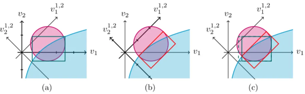
The key idea for the propagation scheme is to interleave the refined Floyd-Warshall algorithm and the constraint propagators. A pseudocode is given on figure 2. At the first level, the DBM is recursively visited so that the minimal bounds for the rotated domains are computed. Each time a DBM cell is modified, the corresponding propagators are added to the propagation list. The propaga-tion list is applied before each new round in the DBM (so that a cell that would be modified twice is propagated only once). The propagation is thus guided by the additional information of the relational domain. This is illustrated on Figure 3: the propagators ρC1...ρCp, ρC1,21 ...ρC
n−1,n
p are first applied (3(a), 3(b)), then
the boxes are made consistent wrt each other using the refined Floyd-Warshall algorithm.
v1 v2 v 1,2 1 v21,2 (a) v1 v2 v 1,2 1 v21,2 (b) v1 v2 v 1,2 1 v21,2 (c)
Fig. 3.Example of the Oct-consistency: an usual consistency algorithm is applied in each basis (Figures 3(a) and 3(b)) then the different boxes are made consistent using the modified Floyd-Warshall algorithm (Figure 3(c)).
We show here that the propagation as defined on figure 2 computes the consistent octagon for a sequence of constraints.
Proposition 4 (Correctness). Let < v1...vn, D1...Dn, C1...Cp > a CSP.
As-sume that, for all i, j ∈ {1...n}, there exists a propagator ρCfor the constraint C,
such that ρC reaches Hull consistency, that is, ρC(D1× ... × Dn) is the Hull
con-sistent box for C. Then the propagation scheme as defined on figure 2 computes the Oct-consistent octagon for C1...Cp.
Proof. This derives from proposition 3, and the propagation scheme of figure 2. The propagation scheme is defined so as to stop when propagList is empty. This happens when ∀i, j ∈ {1...n}, k ∈ {1...2n}, dbm[2i − 1, k]+dbm[k, 2j − 1], dbm[2i − 1, 2i]+dbm[2j, 2j − 1] ≥ dbm[2i − 1, 2j − 1], the same holds for dbm[2i − 1, 2j], dbm[2i, 2j − 1], and dbm[2i, 2j]. The octagonal constraints are thus consistent. In addition, each time a rotated box is modified in the DBM, its propagators are added to propagList. Hence, the final octagon is stable by the application of all ρCi,j
k , for all k ∈ {1...p} and i, j ∈ {1...n}. By hypothesis,
the propagators reach consistency, the boxes are thus Hull-consistent for all the (rotated and regular) constraints. By proposition 3, the returned octagon is
Oct-consistent. ⊓⊔
The refined Floyd-Warshall has a time complexity of O(n3). For each round
in its loop, in the worst case we add p propagators in the propagation list. Thus the time complexity for the propagation scheme of figure 2 is O(n3p3). In the end, the octagonal propagation uses both representations of octagons. It takes advantage of the relational property of the octagonal constraints (Floyd-Warshall), and of the usual constraint propagation on boxes (propagators). This comes to the cost of computing the octagon, but is expected to give a better precision in the end.
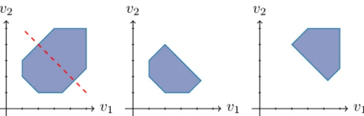
v1 v2 v1 v2 v1 v2
Fig. 4.Example of a split: the octagon on the left is cut in the B1,2basis.
5
Solving
Besides the expected gain in precision obtained with octagon consistency, the box representation of octagons allows us to go a step further and define a fully octagonal solver. We thus define an octagonal split, in order to be able to cut the domains in any octagonal direction, and an octagonal precision, and end up with a fully octagonal solver.
5.1 Octagonal Split
The octagonal split extends the usual split operator to octagons. Splits can be performed in the canonical basis, thus being equivalent to the usual splits, or in the rotated basis. It can be defined as follow:
Definition 9. Given an octagonal domain defined with the box representation D1...Dn, D11,2...Dn−1,n1 ...Dnn−1,n, such that D
i,j
k = [a, b], a splitting operator for
variable vi,jk , computes the two octagonal subdomains D1...[a, (a + b)/2]...Dnn−1,n
and D1...[(a + b)/2, b]...Dn−1,nn .
As for the usual split, the union of the two octagonal subdomains is the original octagon, thus the split does not lose solutions. This definition does not take into account the correlation between the variables of the different basis. We take advantage again of the octagonal representation to communicate the domain reduction to the other basis. A split is thus immediately followed by a Floyd-Warshall propagation. Figure 4 shows an example of the split.
5.2 Precision
In most continuous solvers, the precision is defined as the size of the largest domain. For octagons, this definition leads to a loss of information because it does not take into account the correlation between the variables and domains. Definition 10. Let O be an octagon, and I1...In, I11,2...Inn−1,n its box
represen-tation. The octagonal precision is τ (O) = min1≤i,j≤n(max1≤k≤n(Iki,j− I i,j k )).
Octogone oct
queue splittingList ← oct/*queue of the octagons*/ list acceptedOct ← ∅/*list of the accepted octagons*/ whilesplittingList 6= ∅ do
Octogone octAux ← splittingList.top() splittingList.pop()
octAux ← Oct-consistence(octAux)
if τOct(octAux) < r or octAux contains only solutions then
addoctAux to acceptedOct else
Octogone leftOct ← left(octAux)/*left and right are the split operators*/ Octogone rightOct ← right(octAux)
addleftOct to splittingList addrightOct to splittingList end if
end while
return acceptedOct
Fig. 5.Solving with octagons.
For a single regular box, τ would be the same precision as usual. On an octagon, we take the minimum precision of the boxes in all the bases because it is more accurate, and it allows us to retrieve the operational semantics of the precision, as shown by the following proposition: in an octagon of precision r overapproximating a solution set S, every point is at a distance at most r from S.
Proposition 5. Let < v1...vn, D1...Dn, C1...Cp> be a CSP, and O an octagon
overapproximating S. Let r = τ(O). Let (v1, ...vn) ∈ Rn be a point of D1× ... ×
Dn. Then ∀1 ≤ i ≤ n, mins∈S|vi− si| ≤ r, where s = (s1...sn). Each coordinate
of all the points in O are at a distance at most r of a solution.
Proof. By definition 10, the precision r is the minimum of some quantities in all the rotated basis. Let Bi,j be the basis that realizes this minimum. Because the
box Bi,j = D
1× ... × Di,ji × ...D i,j
j ... × Dn is Hull-consistent by proposition 3,
it contains S. Let s ∈ S. Because r = maxk(Dk− Dk), ∀1 ≤ k ≤ n, |sk− vk| ≤
Dk− Dk≤ r. ⊓⊔
5.3 Octagonal Solver
Figure 5 describes the octagonal solving process. By proposition 4, and the split property, it returns a sequence of octagons whose union overapproximate the solution space. Precisely, it returns either octagons for which all points are solutions, or octagons overapproximating solution sets with a precision r.
An important feature of a constraint solver is the variable heuristic. For con-tinuous constraints, one usually choose to split the variable that has the largest domain. This would be very bad for the octagons, as the variable which has the
largest domain is probably in a basis that is of little interest for the problem (it probably has a wide range because the constraints are poorly propagated in this basis). We thus define a default octagonal strategy which relies on the same remark as for definition 10: the variable to split is the variable Vki,j which realizes the minimum of min1≤i,j≤n(max1≤k≤n(Di,jk − Di,jk )). The strategy is
the following: choose first a promising basis, that is, a basis in which the boxes are tight (choose i, j). Then take the worst variable in this basis as usual (choose k).
6
Experiments
This section compares the octagonal solver with a traditional interval solver on classical benchmarks.
6.1 Implementation
We have implemented a prototype of the octagonal solver, with Ibex, a C++ library for continuous constraints [4]. We use the Ibex implementation of HC4-Revise [3] to contract the constraints. The octagons are implemented with their DBM representation. Additional rotated variables and constraints are posted and dealt with as explained above.
An important point is the rotation of the constraints. The HC4 algorithm is sensitive to multiple occurrences of the variables, and the symbolic rewriting de-fined in section 3.2 creates multiple occurrences. Thus, the HC4 propagation on the rotated constraints could be very poor if performed directly on the rotated constraints. It is necessary to simplify the rotated constraints wrt the number of multiple occurrences for the variables. We use the Simplify function of Math-ematica to do this. The computation time indicated below does not include the time for this treatment, however, it is negligible compared to the solving times. The propagator is an input of our method: we used a standard one (HC4), but more recent propagator such as [1] will be considered in the future. It is sufficient for our needs that the consistency algorithms computes overapproximations of the Hull-consistent boxes, as it is often the case for continuous propagators. 6.2 Results
We have tested the prototype octagonal solver on problems from the Coconut benchmark2. These problems have been chosen depending on the type of the
constraints (inequations, equations, or both).
Experiments have been made, with Ibex 1.18, on a MacBook Pro Intel Core 2 Duo 2.53 GHz. Apart from the variable heuristic presented in subsection 5.3, the experiments have been done with the same configuration in Ibex, in partic-ular, using the same propagators, so as to compare exactly the octagonal results
First solution All the solutions In Oct In Oct h75 41.40 1 0.03 1 >3 hours >3 hours 5 ≤ 1 024 085 149 hs64 0.01 1 0.05 1 >3 hours >3 hours 3 ≤ 217 67 h84 5.47 1 2.54 1 >3 hours 7238.7410 214 322 5 ≤ 87 061 1 407 22 066 421 KinematicPair 0.00 1 0.00 1 53.09 424 548 16.56 39 555 2 ≤ 45 23 893 083 79 125 pramanik 28.84 1 0.16 1 193.14 145 663 543.46 210 371 3 = 321 497 457 2 112 801 1 551 157 trigo1 18.93 1 1.38 1 20.27 12 28.84 347 10 = 10 667 397 11 137 5 643 brent-10 6.96 1 0.54 1 17.72 854 105.02 142 10 = 115 949 157 238 777 100 049 h74 305.98 1 13.70 1 1 304.23 183 510 566.31 700 669 5 = ≤ 8 069 309 138 683 20 061 357 1 926 455 fredtest 3 146.44 1 19.33 1 >3 hours >3 hours 6 = ≤ 29 206 815 3 281
Table 1.Results on problems from the Coconut benchmark. The first column gives the name of the problem, the number of variable and the type of the constraints. In each cell, the number on the left is the CPU time in seconds. Upper right is the number of box in the computed solution, lower right the number of created boxes.
with their interval counterparts. Table 1 compares the results obtained by the interval resolution to those obtained by the octagonal resolution. In the first four problems the constraints are inequalities, in the three following they are only equalities and in the last two they are mixed inequalities and equalities. The octagonal solver needs less time and created less boxes to find the first solu-tion of a problem. We obtain better results on problems containing inequalities. Problems with equalities contain multiple occurrences of variables, which can explain the bad results obtained by the octagonal solver on those problems.
7
Related Works
Our work is related to [9], in static analysis of programs. Their goal is to compute overapproximations for the traces of a program. The octagons are shown to provide a good trade off between the precision of the approximation and the computation cost. We use their matrix representation and their version of the Floyd-Warshall algorithm.
Propagation algorithms for the difference constraints, also called temporal, have already presented in [5, 11]. They have a better complexity than the one we use, but are not suited to the DBM case, because they do not take into account the doubled variables.
The idea of rotating variables and constraints has already been proposed in [7], in order to better approximate the solution set. Their method is dedicated to under-constrained systems of equations.
8
Conclusion
In this paper, we have proposed a solving algorithm for continuous constraints based on octagonal approximations. Starting from the remark that domains in Constraint Programming can be interpreted as components of a global multi-dimensional parallelepipedic domain, we have constructed octagonal approxi-mations on the same model and provided algorithms for octagonal CSP trans-formations, filtering, propagation, precision and splitting. An implementation based on Ibex and preliminary experimental results on classical benchmarks are encouraging, particularly in the case of systems containing inequalities. Future work involves the experimental study of other interval-based propagators such as Mohc [1] and extensions to other geometric structures.
References
1. Ignacio Araya, Gilles Trombettoni, and Bertrand Neveu. Exploiting monotonicity in interval constraint propagation. In Proceedings of the 24th AAAI Conference on Artificial Intelligence, AAAI 2010, 2010.
2. Fr´ed´eric Benhamou. Heterogeneous constraint solvings. In Proceedings of the 5th International Conference on Algebraic and Logic Programming, pages 62–76, 1996. 3. Fr´ed´eric Benhamou, Fr´ed´eric Goualard, Laurent Granvilliers, and Jean-Fran¸cois Puget. Revisiting hull and box consistency. In Proceedings of the 16th International Conference on Logic Programming, pages 230–244, 1999.
4. Gilles Chabert and Luc Jaulin. Contractor programming. Artificial Intelligence, 173:1079–1100, 2009.
5. Rina Dechter, Itay Meiri, and Judea Pearl. Temporal constraint networks. In Proceedings of the first international conference on Principles of Knowledge Rep-resentation and Reasoning, 1989.
6. Robert Floyd. Algorithm 97: Shortest path. Communications of the ACM, 5(6), 1962.
7. Alexandre Goldsztejn and Laurent Granvilliers. A new framework for sharp and efficient resolution of ncsp with manifolds of solutions. In Proceedings of the 14th international conference on Principles and Practice of Constraint Programming (CP ’08), pages 190–204, Berlin, Heidelberg, 2008. Springer-Verlag.
8. Miguel Menasche and Bernard Berthomieu. Time petri nets for analyzing and ver-ifying time dependent communication protocols. In Protocol Specification, Testing, and Verification, 1983.
9. Antoine Min´e. The octagon abstract domain. Higher-Order and Symbolic Compu-tation, 19(1):31–100, 2006.
10. Ramon Moore. Interval Analysis. Prentice-Hall, Englewood Cliffs N. J., 1966. 11. Jean-Charles R´egin and Michel Rueher. Inequality-sum : a global constraint
cap-turing the objective function. RAIRO Operations Research, 2005.
12. Christian Schulte and Peter J. Stuckey. Efficient constraint propagation engines. Transactions on Programming Languages and Systems, 31(1):2:1–2:43, December 2008.