Titre:
Title
:
A framework to compute statistics of system parameters from very
large trace files
Auteurs:
Authors
: Naser Ezzati-Jivan et Michel R. Dagenais
Date: 2013
Type:
Article de revue / Journal articleRéférence:
Citation
:
Ezzati-Jivan, N. & Dagenais, M. R. (2013). A framework to compute statistics of system parameters from very large trace files. ACM SIGOPS Operating Systems
Review, 47(1), p. 43-54. doi:10.1145/2433140.2433151
Document en libre accès dans PolyPublie
Open Access document in PolyPublie
URL de PolyPublie:
PolyPublie URL: https://publications.polymtl.ca/2954/
Version: Version finale avant publication / Accepted versionRévisé par les pairs / Refereed Conditions d’utilisation:
Terms of Use: Tous droits réservés / All rights reserved
Document publié chez l’éditeur officiel
Document issued by the official publisher
Titre de la revue:
Journal Title: ACM SIGOPS Operating Systems Review (vol. 47, no 1)
Maison d’édition:
Publisher: ACM
URL officiel:
Official URL: https://doi.org/10.1145/2433140.2433151
Mention légale:
Legal notice:
© 2013. This is the author's version of the work. It is posted here for your personal use. Not for redistribution. The definitive Version of Record was published in ACM SIGOPS Operating Systems Review, https://doi.org/10.1145/2433140.2433151."
Ce fichier a été téléchargé à partir de PolyPublie, le dépôt institutionnel de Polytechnique Montréal
This file has been downloaded from PolyPublie, the institutional repository of Polytechnique Montréal
A FRAMEWORK TO COMPUTE STATISTICS OF SYSTEM PARAMETERS FROM VERY
LARGE TRACE FILES
Naser Ezzati-Jivan
[email protected]
Michel R. Dagenais
[email protected]
Department of Computer and Software Engineering
Ecole Polytechnique de Montreal
Montreal, Canada
ABSTRACT
In this paper, we present a framework to compute, store and retrieve statistics of various system metrics from large traces in an efficient way. The proposed framework allows for rapid interactive queries about system metrics values for any given time interval. In the proposed framework, efficient data struc-tures and algorithms are designed to achieve a reasonable query time while utilizing less disk space. A parameter termed gran-ularity degree (GD) is defined to determine the threshold of how often it is required to store the precomputed statistics on disk. The solution supports the hierarchy of system resources and also different granularities of time ranges. We explain the architecture of the framework and show how it can be used to efficiently compute and extract the CPU usage and other system metrics. The importance of the framework and its dif-ferent applications are shown and evaluated in this paper.
Index Terms— trace, statistics, system metrics, trace ab-straction, Linux kernel
1. INTRODUCTION AND PROBLEM STATEMENT The use of execution traces is increasing among system ad-ministrators and analysts to recognize and detect problems that are difficult to reproduce. In a real system, containing a large number of running processes, cores and memory mod-ules, when a runtime problem occurs(e.g. a performance degra-dation), it may be difficult to detect the problem and discover its root causes. In such a case, by instrumenting the operat-ing system and applications, tracer tools can provide valuable clues for diagnosing these failures.
Although trace information provides specifics on the sys-tem’s runtime behavior, its size can quickly grow to a large number of events, which makes analysis difficult. Thus, to facilitate analysis, the size of large traces must somehow be reduced, and high level behavior representation must be ex-tracted. Trace abstraction techniques [1, 2, 3] are used to re-duce the size of large traces by combining and replacing the
raw trace events with high level compound events. By us-ing trace abstraction, it is possible to create a hierarchy of high level events, in which the highest level reveals general behaviors, whereas the lowest level reveals more detailed in-formation. The highest level can start with the statistics view. This statistics view can be used to generate measurements of various system metrics, and create the general overview of a system execution in the form of histograms or aggregated counts. It is also possible to use other mechanisms (e.g. navi-gation and linking) to focus on a selected area, go deeper, and obtain more details and information.
Statistics play a significant role in every field of system analysis, especially in fault and attack detections. The overview of different system parameters, such as the CPU load, num-ber of interrupts, IO throughput, failed and successful net-work connections, and number of attack attempts can be used in various applications that range from optimization, resource utilization, bottleneck, fault and attack detection to even bench-marking and system comparisons. In short, inspecting the statistics of several system metrics may be used in the earlier steps of any trace based system analysis.
Since the statistics computation may be used interactively and frequently for large traces, it is worth having efficient data structures and algorithms to compute system metrics statistics and parameters. These data structures and algorithms must be optimized in terms of construction time, access time and required storage space.
The simplistic solution for providing the required statis-tics is to take a trace, read the events of the given interval, and compute the desired statistics. However, it is not recom-mended to have the trace events read each time, especially when the trace size is large, as reading trace events of large intervals is inefficient, and may waste valuable analysis time. The problem of statistics computation in general faces two main challenges: first, the difficulty of efficiently computing the system metrics statistics without having to reread the trace events; and second, finding a way to support large traces. In other words, on one hand, the challenge lies in finding a way
to compute -in a constant time- the statistics of various sys-tem metrics for any arbitrary time interval, without rereading the events of that interval (e.g. computing the system metrics statistics of a 20 GB interval in a 100 GB trace short of reread-ing that particular 20 GB of the trace). On the other hand, the next challenge then becomes providing a scalable architec-ture to support different trace sizes (from a few megabytes to over a terabyte of trace events), and at the same time, different types of statistics and hierarchical operations.
In this paper, we propose a framework for incrementally building a scalable metrics history database to store and man-age the precomputed system metrics values, used to rapidly compute the statistics values of any arbitrary intervals.
The framework is designed according to the following cri-teria:
1. performance, in terms of efficiency in statistics compu-tation and query answering algorithms,
2. compactness, in terms of space efficiency of the data structures and finally,
3. flexibility, in terms of supporting different system met-rics (e.g. IO throughput, CPU utilization, etc.), and hi-erarchy operations for different time scales (i.e. mil-lisecond, second, minute and hour) and system resources (e.g. a process, a group of processes, a virtual machine, or the whole system).
To test the proposed data structures and algorithms, we use kernel traces generated by Linux Trace Toolkit next gen-eration (LTTng) [4]. LTTng is a low impact, precise and open source Linux tracing tool that provides detailed exe-cution tracing of operating system operations, system calls, and user space applications [4]. By evaluating the resulting trace events, this method automatically draws an overview of the underlying system execution, based on a set of prede-fined metrics (e.g. number of bytes read and written), which can then be used to detect system problems and misbehaviors caused by program errors, an application’s misconfiguration or even attacks. Further investigations may lead to oppor-tunity to apply some administrative responses to solve those detected problems [5].
The remainder of the paper is organized as follows: first, we present the architecture of the statistics framework, and the details of its different modules. Secondly, we present an example highlighting the use of the proposed framework, and subsequent data structures and algorithms. Then, we discuss our experiences and evaluation of the proposed method. Fi-nally, we conclude by outlining specific areas of investigation for future enhancements.
2. RELATED WORK
Bligh et al. [6] use kernel trace data to debug and discover in-termittent system problems and bugs. They discuss the
meth-ods involved in debugging the Linux kernel bugs to find real system problems like inefficient cache utilization and poor la-tency problems. The interesting part is that for almost all in-vestigated problems, inspecting the statistics of system met-rics is the starting point of their analysis. Using trace data to detect and analyze the system problems also mentioned in [7, 8, 9]. Xu et al. [7] believe that system level performance indicators can denote high level application problems. To ad-dress such problems, Cohen et al. [9] first established a large number of metrics such as CPU utilization, I/O requests, aver-age response times and application layer metrics. They then related this metrics to the problematic durations (e.g. dura-tions with a high average response time) to find a list of met-rics, indicative of these problems. The relations that Cohen et al. discovered can be used to describe each problem type in terms of a set of metrics statistics [8]. They denoted how to use statistics of system metrics to diagnose system problems. However, they do not consider scalability issues, where the traces are too large and where the storing and retrieving of statistics are key challenges.
Some research uses the checkpoint or periodic snapshot method to collect and manage the system statistics [10, 11]. This method splits the input trace into equal parts (e.g. a checkpoint for each 100 K events), and stores the aggregated information from each checkpoint in a memory based database. After reading a trace and creating the checkpoint database, for computing statistics of any given time point, the method ac-cesses the previous checkpoint, rereads and reruns the trace from the previous checkpoint up to the given point, and com-putes the desired statistics. Kandula et al. [10] store snap-shots of the system configurations in order to analyze how each component depends on the network system, and to de-termine the main cause of each system fault. LTTV (a LTTng viewer) and TMF (Tracing and Monitoring Framework)1use the checkpoint method for extracting system state values at any given time point.
Although the checkpoint method is considered a useful solution for managing the statistics, it requires rereading the trace and does not support the direct computation of statistics found between two checkpoints. Moreover, different metrics with varying incident frequencies (e.g. number of events vs number of multi step attacks) are treated in the same way. In other words, since the method uses equal size checkpoints for the metrics that have trifle value changes during a system ex-ecution, loading a checkpoint and rereading the trace to com-pute its statistics at different points may waste time, and not produce any values. In the same way, metrics with large in-cidents, demand more effort to recompute the required statis-tics. In this paper, we will show that creating variable length checkpoints for different metrics leads to better construction and access performance.
The checkpoint method uses memory-based data struc-tures to store the checkpoint values. However, using a
based database imposes a strict limit on the trace size that can be supported. The same problem exists for other interval man-agement data structures like the Tree-Based Statistics Access Method (TBSAM) [12], segment-tree, interval-tree, Hb-tree, R-tree (and its variants R+-tree and R*-tree), etc. [13]. Seg-ment tree and interval tree work properly for static data sets, but do not work well for incrementally built intervals, because they lead to performance degradation. Likewise, the R-tree and its extensions do not work well for managing interval se-quences that have long durations, and are highly overlapped, as indicated in [14]. Furthermore, the splitting and merging (rebalancing) of the nodes drive many changes in the pointers, inducing severe performance degradation.
In the DORSAL lab2, co-workers Montplaisir et al. [15] introduced an external memory-based history tree for storing the intervals of system state values. In their history tree, sys-tem state values are modeled as intervals. Each interval in this tree contains a key, a value, a start and an end time. The key represents a system attribute whose state value is stored in this interval. The start and end times represent the start-ing and endstart-ing points of the given state value. In this tree each node corresponds to a time range and contains a bucket of intervals lying within the node’s time range. Since they use a disk-based data structure to store the state information, the solution is scalable, and successfully tested for traces up to 1 TB, yet is optimized for interval queries, and has a fast query time. It takes O(log(n)) time (i.e. n equals the number of nodes) to perform a stabbing query to locate and extract a state value from the data store. The tree is created incremen-tally in one pass of the trace reading. The nodes have a pre-defined fixed size in the disk. Whenever a node becomes full, it is marked as ”closed”, and a new node is created. For that reason, it does not require readjustment as seen in the R-tree and its variants. Montplaisir et al. reported that they could achieve a much better query performance than the LTTV3, TMF, R-tree and PostgreSQL database system [15].
They have designed that solution to store and manage the modeled state, but have not studied and optimized it for the statistics. Although the history tree, as they report, is an ef-ficient solution for managing the state values, it can not be used directly in the statistics framework, as if it stores met-rics as state, every increment will become a state change in an interval tree, which wastes much storage space. Our ex-periment shows that in this case the size of the interval tree is comparable to the original trace size, which is not reasonable. Although their partial history tree approach [15] works like a checkpoint mechanism, and solves the storage problems, the query time remains a problem, since it must access the original traces to reread and recompute the statistics for the points lying between two checkpoints; that could be a time-consuming task for large checkpoints. Despite the same idea of handling the value changes as intervals behind both the
2http://www.dorsal.polymtl.ca/ 3http://lttng.org/lttv
history tree and the proposed framework, there are major dif-ferences that are explained in the following:
1. Granularity degree (GD) is introduced to make the data structure as compact as possible,
2. Different organization of the system resources and met-rics is used to avoid duplication in the interval tree struc-ture.
3. Rereading and reprocessing the the trace events is avoided. Instead, the interpolation technique is used to calculate the half-way values.
3. GENERAL OVERVIEW OF THE SOLUTION Kernel tracing provides low-level information from the op-erating system execution that can be used to analyze system runtime behavior, and debug the execution faults and errors that occur in a productive environment. Some system run-time statistics can be extracted using system tools like prstat, vmtree, top and ps, however, these tools are not usually able to extract all the important information, necessary for a com-plete system analysis. For instance, they do not contain the operation timestamps, nor always the owning process infor-mation (e.g. which process has generated a packet), both of which are important in most system analysis. This informa-tion can be extracted from a kernel trace. Kernel traces usu-ally contain information about [16]:
• CPU states and scheduling events, can be used to cal-culate the CPU utilization;
• File operations like open, read, write, seek and close, can be used to reason about file system operations and extract IO throughput;
• Running processes, their execution names, IDs, parent and children;
• Disk level operations, can be used to gather statistics of disk access latencies;
• Network operations and the details of network packets, can be used to reason about network IO throughput and network faults and attacks;
• Memory management information like allocating or re-leasing a memory page, can be used to obtain and ana-lyze the memory usages.
Since the kernel trace contains valuable information about the underlying system execution, having a mechanism to ex-tract and render statistics of various system metrics, based on system resources and time data, can be helpful in finding sys-tem runtime problems and bugs. By providing such a statis-tics view, the trace analysis can start with an overview of the
system, and continue by zooming in on the strange and abnor-mal behaviors (e.g. spikes in a histogram view) to gain more information and insight.
By processing the trace events, one can compute impor-tant system metrics statistics, and aggregate them per ma-chine, user, process, or CPU for a whole trace or for a specific time range (e.g. for each second). The following are exam-ples of statistics that can be extracted from a kernel trace:
• CPU time used by each process, proportion of busy or idle state of a process.
• Number of bytes read or written for each/all file and network operation(s), number of different accesses to a file.
• Number of fork operations done by each process, which application/user/process uses more resources.
• Which (area of a) disk is mostly used, what is the la-tency of disk operations, and what is the distribution of seek distances.
• What is the network IO throughput, what is the number of failed connections.
• What is the memory usage of a process, which number of (proportion of) memory pages are (mostly) used. Although each trace contains a wealth of information, it is not always easy to extract and use it. The first problem is size of the trace. A large trace usually complicates the scalable reading and analysis. Another problem is that the statistics information is also not clearly displayed, and is hidden be-hind millions of events. This means the trace events have to be analyzed deeply to extract the desired statistics. Moreover, since the statistics computation will be used widely during system analysis, it must be fast and efficient enough to extract the desired analysis on demand. Therefore, tools and algo-rithms must be developed to deal with these problems.
In this paper, we propose a framework that efficiently pro-vides statistical information to analysts. The framework works by incrementally building a tree-based metric data store in one pass of trace reading. The data store is then used at analysis time to extract and compute any system metrics statistics for any time points and intervals. Using a tree-based data store enables the extraction and computation of statistics values for of any time range directly, without going through the relevant parts in the original trace. Such a data store also provides an efficient way to generate statistics values from a trace, even if it encompasses billions of events. The architecture, algo-rithms and experimental results will be explained in the fol-lowing sections.
This framework also supports hierarchical operations (e.g. drill down and roll up) among system resources (i.e. CPU, process, disk, file, etc.). It enables gathering statistics for a
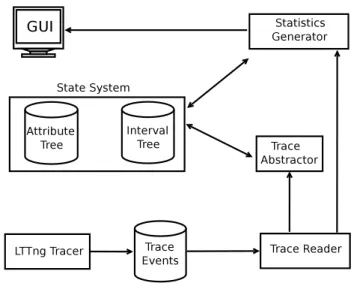
Fig. 1: General architecture of the framework.
resource, and at the same time, for a group of resources (e.g. IO throughput for a specific process, for a group of processes, or for all processes). Furthermore, it supports different time scales, and it is possible to zoom in on the time axis to retrieve statistics for any time interval of interest.
The framework we propose also supports both online and offline tracing. In both cases, upon opening a trace, the frame-work starts to read and scan the trace events, precompute the predefined metric values, and store in the aforementioned in-terval history data store. Whenever an analysis is needed, it queries the data store, extracts the desired values and com-putes the statistics. With this system, users can go back to retrieve the statistics from any previous points of system exe-cution.
4. ARCHITECTURE
In this section, we propose the architecture of a framework for the live statistics computation of system metrics. The solution is based on incrementally building a metrics history database to be used for computing the statistics values of any arbitrary intervals in constant time. Constant time here means the dependence of the computation time on the length of the in-terval. It works by reading trace events gathered by the LT-Tng kernel tracer and precalculating and storing values of the prespecified system metrics at different points in a tree-based data structure. Using tree-based data structures enables an efficient access time for large traces. Figure 1 depicts a gen-eral view of the framework architecture, covering its different modules.
As shown in Figure 1, this architecture contains differ-ent modules such as trace abstraction, data store and statistics generation, which are explained in the following sections:
Kernel Tracer: LTTng
We use the LTTng [4] kernel tracer to trace operating system execution. LTTng is a powerful, low impact and lightweight [17] open source Linux tracing tool, and provides precise and detailed information of underlying kernel and user space ex-ecutions. LTTng contains different trace points in various modules of the operating system kernel, and once a prede-fined trace point is touched, it generates an event containing a time-stamp, CPU number and other information about the running process. Finally, it adds the event to an in-memory buffer to be stored later on disk [4].
Trace Abstractor
The trace size is usually very large that makes difficult to an-alyze and understand the system execution. Most of the time another analysis tool is required to abstract out the raw events and represent them with higher-level events, reducing the data to analysis. Trace abstraction is typically required to com-pute statistics of complex system metrics that are not directly computable from the raw trace events. For instance, to com-pute synthetic metrics statistics like ”number of HTTP con-nections”, ”CPU usage”, and ”number of different types of system and network attacks”, raw events must be aggregated to generate high-level events; then, the desired statistics must be extracted and computed. The details of the trace abstrac-tion tool we use to generate such high level meaningful events from raw events, may be found in [2]. In the remainder of this text, the term event is used to refer to both raw and abstract events.
State System
The state system is a database used for managing the state val-ues of a system at different points. Examples of state valval-ues are: execution status of a process (running, blocked, waiting), mode of a CPU (idle, busy), status of a file descriptor (opened, read, closed), disks, memory, locks, etc.
State values are extracted from trace events based on a predefined mapping table. In this table, there is an entry spec-ifying how an event can affect the value of a resource state. For example, the state of a process (whether it is running or blocked) can be extracted using CPU scheduling events.
In the DORSAL lab4, Montplaisir et al. [15] introduced a tree-based data structure, called state history tree, which stores and retrieves the system state values. In their history tree, system state values are modeled as intervals and each in-terval contains complete information about a state value change. For instance, when the state of a process is changing from ready to running, an interval is created in the history tree, specifying start and end points of the change, the process name and the state value.
4http://www.dorsal.polymtl.ca/
The state system proposed in [15] uses two mechanisms for managing the state values:
• partial history tree, that makes use of a method simi-lar to the checkpoint method, to store and manage the state values. In this system, for extracting state of any halfway points laying between two checkpoints, it is required to access the trace events to reread, rerun and extract the state value. However, another access and reread the trace, may waste time. In our method, we read the trace once and will not refer to it again. • complete history tree, that stores every change of state
values and extracts directly any required state value. Although it extracts the state values directly without rereading the trace, the method needs lots of storage space. Experiment results show that in some occasions, related to the number of active system resources, it needs a storage space larger than the original trace size. How-ever, since the statistics may be used widely in the sys-tem, we need a compact data store, and at the same time, a faster access time.
Managing the statistics values of different system metrics can be implemented using the same mechanism as what is used for managing the states. Although the history tree intro-duced in [15] is an efficient solution for managing the state changes, it still needs some modifications to be used here in the statistics framework. In Montplaisir et al.’s work, any value change of the system state is stored in a separate in-terval. However, storing all statistics value changes in the interval tree will waste much storage space. As explained, our experiment shows that the size of the interval tree, in this case, will be comparable to the original trace size. Although using their partial history tree [15] that works like checkpoint mechanism, solves the storage problems, the query time re-mains a problem. What we look for here is a compact data store and efficient algorithms to directly compute the system metrics statistics, without having to reread and rerun the trace events.
5. STATISTICS GENERATOR
The statistics generator, the main module of the framework, is responsible for computing, storing and retrieving the statistics values. Since in the kernel traces all data comes in the form of trace events, a mapping table is needed to extract quanti-tative values from the events. Similar to the event-state map-ping, the statistics module uses an event-statistics mapping table that identifies how to compute statistics values from the trace events. In this table, there exists an entry that speci-fies which event types, and their subsequent payload are re-quired for extracting metric statistics. For instance, for com-puting the number of ”disk IO throughput”, file read and write events are registered. In the same way, the ”HTTP connec-tion” abstract events are counted to compute the number of
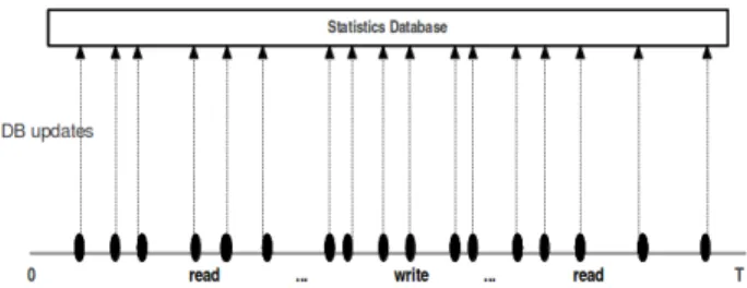
Fig. 2: Database updates for granularity degree = 1.
failed/successful HTTP connections. The former is an exam-ple of a basic metric, computed using the raw events directly. However, the latter is an example of a synthetic metric, com-puted using outputs of the abstracter module.
In this framework, we store the statistics values in interval form. To do so, in the trace reading phase the duration of any value change in a system metric is considered an interval, and is stored in the data store. The time-stamp of the first event (registered to provide values of the metric) is considered the starting point of the interval. In the same way, the time-stamp of the next value change is considered the end point of that interval. Similarly, any other value change is kept in an other interval.
The parameter ”granularity degree” (GD) is defined to de-termine how often the computed statistics of a metric should be stored in the database. It does not however affect the com-putation frequency of a metric. Comcom-putation is accomplished any time a relevant event occurs, and is independent of the granularity degree. The granularity degree can be determined using the following different units:
• Counts of events (e.g. each 100 events).
• Counts of a specific event type (e.g. all scheduling events);
• Time interval (e.g. each second).
For instance, when one assigns a granularity degree , say k, to a metric he or she has already specified the frequency of updates in the database. In this case, for each k changes in the statistics value, an update will be accomplished in the database. There is a default value for the granularity degree but it can be adjusted separately for each metric. Figure 2 shows updates for a case in which the granularity degree is one, while Figure 3 shows the number of updates for a larger granularity degree.
Using the notion of granularity degree leads to a faster trace analysis, data store construction, and also a better query answering performance. The efficiency increases because with a large granularity degree, less information will be written to disk.
Fig. 3: Database updates for granularity degree = 5.
Fig. 4: Using linear interpolation to find a halfway value.
Although defining a proper granularity degree leads to a better construction and access time, it may require additional processing to answer queries for the halfway points, lead-ing to search performance degradation, particularly when the granularity degree is coarser than the query interval range. In this case there are two solutions to compute the desired statis-tics: rereading the trace or using the interpolation technique.
The first solution is similar to the checkpoint method, which rereads the trace to computes the desired statistics. This tech-nique is also used in the partial history tree proposed by Mont-plaisir et al. [15]. Although this solution works well for small traces, it is not a great idea to reread the trace and reextract the values, each time users query the system. Especially when the trace size is large, checkpoint distances are large, and the system load is high.
The second solution is to use the interpolation technique. Using linear interpolation, as shown in Figure 4, makes pos-sible to find any halfway values within two extremes of the granularity checkpoints, without rereading the trace events.
Figure 5 shows an example of statistics computation using both the interpolation technique and the granularity degree parameter. In this example, the goal is to find the statistics of a particular metric between two points A, B in the trace. The bold points show the borders of the GD durations and there is one data structure update for each point.
V alAB = V alB− V alA= x1 + x2 + x3 (1) The value of x2 can be computed using the subtraction of the two values in t2 and t3. However, since the x1 and x2 are half values between two updates (inside a GD), they can be computed using the interpolation technique, as denoted in the Formula 2. One last point is that the values V alt1, V alt2
Fig. 5: Example of using linear interpolation and granularity degree parameter.
and V alt3can be extracted directly from the interval tree data structure using stabbing queries (as will be explained in the next section). x1 = V alt1+ (A − t1) (V alt2− V alt1) (t2 − t1) x2 = V alt3− V alt2 x3 = V alt3+ (B − t3) (V alt4− V alt3) (t4 − t3) (2)
Although the interpolation technique returns an estima-tion of the real value, there may be doubts about its preci-sion. The precision of the result actually depends on the size of granularity degree. In other words, by carefully adjusting the granularity degrees for different metrics according to their importance, it is possible to estimate a fairly accurate results. For instance, by determining small numbers for less precise metrics (e.g. CPU utilization for evaluating the affinity of a scheduling algorithm) and relatively large values for less pre-cise metrics (e.g. number of trace events), one can achieve better results.
We will continue explaining the architecture with an ex-ample in the next section.
Illustrative Example
In this section, we investigate an example to show how to use the proposed method for computing the statistics of system metrics in a large trace. The example shows how to compute the CPU utilization for different running processes, separately or in a group, during any arbitrary time intervals of the under-lying system execution.
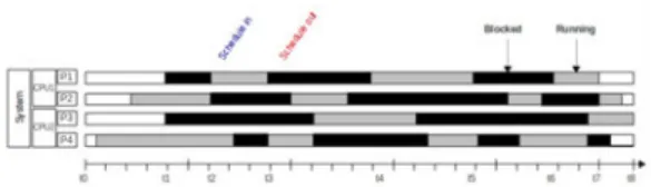
The first step is to specify how the statistics values are ex-tracted from the kernel trace events. We use trace scheduling events to extract the CPU utilization. The scheduling event ar-guments show the CPU number, the process id that acquires the CPU as well as the process that releases the CPU. Utiliza-tion is computed by summing up the length of the duraUtiliza-tions that a CPU is used by a running process. Figure 6 shows a possible case of CPU scheduling for two processors and four processes. In the example shown in Figure 6:
Fig. 6: An example of the CPU scheduling.
CP U1 utilization of running process P1: U (P1)CP U 1= (t3− t2) + (t5− t4) (3) U tilization of CP U1: U (CP U1) = Pi=2 i=1U (Pi)CP U1 t8− t0 (4) And in general:
CP Uk utilization of each running process Pi: U (Pi)CP Uk= Pm,n=te m,n=ts(tm− tn) (5) U tilization of CP Uk : U (CP Uk) = Pi=n i=0U (Pi)CP Uk te− ts = P i Pm,n=te m,n=ts(tm− tn)i te− ts (6)
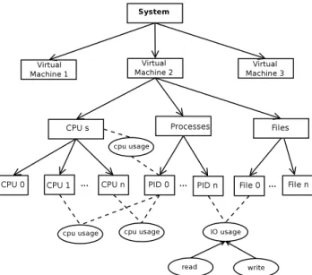
As explained earlier, one of the features of this framework is being able to perform hierarchical queries. To do this, we build a tree called the ”metric tree” containing a hierarchy of resources and metrics. The construction of such a hierar-chy makes it possible to drill down and roll up between the resources, and to aggregate the statistics values for different granularities (e.g. for a process, group of processes, a virtual machine or even for whole system). Figure 7 models a typical organization of the metric tree.
As shown in Figure 7, there are hierarchies of system sources and metrics separately. In this tree the system re-sources (e.g. processes, files, cpus, network ports, etc.) are organized in the separate branches of the tree. Then, the met-rics nodes that could be a tree as well, connect the resources together. For example, the metric ”cpu usage” connects two nodes, a process and a cpu, representing the cpu usage of that process. Each metric node is assigned a unique number that is used as a multivalue key for future references to the cor-responding statistics values in the interval tree. Metric nodes can be used to connect different resources together, individu-ally or in a group. For instance, a IO usage metric may con-nect a process to a particular file or to the files of a folder or even to all files, showing respectively the bytes of this file read or written by that process, the bytes read or written in the files of a folder, or the whole IO of that process. For
Fig. 7: A general view of the metric tree.
each resource, there is a path from the root node. For each metric node, there is at least one path from the root node as well, representing which resources this metric belongs to. In this tree the metrics and the resource hierarchies are known in advance, however, the tree is built dynamically. Organiz-ing the resources and metrics in such a metric tree enables us to answer hierarchical queries like ”what is the CPU us-age (a specific CPU or all of them) of a process (or a group of them)?”, and ”what is the IO throughput of a system, or a group of running processes?”.
This hierarchy of resources facilitates the computing of the hierarchy statistics. For any resources or group of re-sources for which statistics values should be kept, a metric node is created and connects them to the other resource (or group of resources) using a proper key value. For example, when cpu usage of a specific core of a specific process is im-portant, we consider a cpu usage metric node between these two resources and assign a unique key value to that. As an-other example, in addition to the IO usage of the different processes, someone may be interested in monitoring the IO usage of an important file like /etc/passwd since it is accessi-ble by all processes. In this case, it is just required to make a IO usage node, connect that node to that particular file and to the ”Processes node” in the tree, and assign another unique key value to that. This key value is used as a reference to the different statistics values in the interval tree.
The solution is based on reading trace events, extracting the statistics from them, and storing them in the correspond-ing interval database nodes, accordcorrespond-ing to the correspondcorrespond-ing granularity degrees.
After creating a hierarchy of resources and metrics, it is then time to decide how to store and manage the statistics values. As explained earlier, we model the statistics values
Fig. 8: A view of the intervals and the corresponding nodes.
in intervals and store them in a tree-based interval data store. In this data store, data is stored in both the leaf and non-leaf nodes. Each node of the tree contains a bucket of interval entries lying within the range of its time boundaries. A view of this tree and corresponding intervals are shown in Figure 8.
Each interval contains a start time, end time, key and value. The key refers to a metric node in the metric tree. The value shows a cumulative value, from the starting time of the trace to that point. Based on the start and end times, intervals are organized into the minimum containing tree nodes.
The created metric and statistics trees are used to extract the desired statistics in the analysis phase. In other words, computing the statistics of a metric is accomplished by per-forming a stabbing query at any given query point. The stab-bing query returns all the tree nodes intersecting a given time point [18]. The query result is the statistics value of the metric at that given point. In the same way, computing the statis-tics of an interval of interest, instead of a single point, is answered by performing two stabbing queries: one for ex-tracting the aggregated value of the interval start point of the interval, and one for the end point. For each metric, it is rea-sonable to retrieve at most one result per each stabbing query, as only one value for each point or interval has been stored during the event reading time. After performing the stabbing queries for the start and end point of a given interval, the de-sired result is the difference between these two query results. The algorithm is shown in Listing 1. The algorithm takes 2*O(log(n)) time to compute the statistics values of a metric and time range (log(n) for each stabbing query, n is the num-ber of tree nodes). Detailed experiment results will be shown in the next chapter. For each stabbing query, a search is started from the root downward, exploring only the branch and nodes
Algorithm 1 Complete interval query.
Require: a time range [t1 - t2] and v a set of metric keys. 1: set upperBoundV alue = 0;
2: find all nodes of the tree that intersect t2 (stabbing query); 3: search within nodes’ intervals and find all entries that
contain at least one of the metric keys; 4: if found any then
5: for each entry do
6: set upperBoundV alue = upperBoundV alue +
entry.value; 7: end for 8: end if
9: set lowerBoundV alue = 0;
10: find all nodes of the tree that intersect t1 (stabbing query); 11: search within nodes’ intervals and find all entries that
contain at least one of the metric keys; 12: if found any then
13: for each entry do
14: set lowerBoundV alue = lowerBoundV alue +
entry.value; 15: end for 16: end if
17: return upperBoundV alue - lowerBoundV alue;
that possibly contain the given point. Within each node, it it-erates through all the intervals and returns only the entry in-tersecting the given point. Since the intervals are disjoint, the stabbing query will return at most one value. However, it is possible to not find any stabbing interval for the given time point, which means there is no metric value for the given time point, and it will be considered zero.
To traverse the tree, the algorithm performs a binary search on the tree, and copies the resulting branch to the main mem-ory. It then searches the nodes and its containing interval en-tries to find the statistics value of the given metric. In other words, by doing a stabbing query, statistics values of the other metrics which intersect the query point, will also be in the main memory. We call this data set ”current statistics values”. The current statistics values can then be used for computing and extracting the statistics of other system metrics for the same query point. The important point here is that, since the current statistics values data set is in main memory rather than the external disk, performing subsequent queries to compute other metrics statistics for the same query point will be much faster than the base stabbing query.
Hierarchy Operations
As mentioned earlier, the framework supports hierarchical queries between resources. For example, it is possible to compute the CPU utilization of one process, at the same time as a group of
Algorithm 2 Stabbing query.
Require: time point t and the metric name.
search all intervals in the root node to see whether exists any containing interval for the given time point t.
if found then
return the entry value
else {if not found and the node is not a leaf}
find the corresponding child node regarding to the chil-dren intervals and given time point t.
end if
if exists any node then
Perform a query in the subtree that this node is its root. else
return zero end if
processes, or for the whole system.
To support these queries, there are two general approaches in the proposed framework. The first and obvious solution is to separately compute and store the temporary statistics val-ues of each resource (e.g. process, file, CPU, etc.), and all possible groups of resources from the trace events. For in-stance, the count of CPU time for any group of processes, and for the whole system are accumulated separately when rele-vant trace events are received. The problem of this solution is that all groups of processes that will be queried later by an analyst must be known in advance. However, it is not always possible to predict which group of processes an analyst may be interested in. Also, the solution requires much space to store the duplicate values of all resource combinations. More-over, at analysis time, all statistics computations must be an-swered by querying the external interval tree, which is too time consuming.
The second and better solution is to compute the hierarchy statistics values by summing up the children resource statis-tics. For instance, the count of CPU time for any group of processes is extracted by summing up the total CPU time of the group’s children processes. Unlike the previous approach, it is not necessary to know in advance or even to predict the re-source groups that will be inspected by analysts. In this solu-tion, we use the aforementioned current statistics values data set to answer the hierarchical queries. Since all of intersect-ing nodes and intervals will be brought to the main memory upon performing a stabbing query, it is possible to integrate and sum up the statistics values of any system resources to quickly compute the statistics value of a group of resources. Since the current statistics values data set is in main memory, hierarchical queries can be performed quickly.
Using the second approach, for performing a hierarchi-cal query it first find the values of children nodes using the aforementioned stabbing queries, and then, aggregate results to find a value of the desired high level node. Equations 5, 6,
and 7 show relations between a high level statistics value and its containing nodes:
U tilization of all processors : U (All CP U s) =Pj=n j=0U (CP Uj) And totally : =Pj=n j=0 Pi=m i=0 U (Pi)CP Uj te− ts (7)
The CPU utilization of the whole system can be computed by summing up the CPU utilization of each processor sepa-rately, which can be acquired in turn by computing the utiliza-tion of each process by doing two stabbing queries over the disk based interval tree, and consecutively a memory based linear search. In the same way, the same solution can be used for other metrics and resource hierarchies.
The above example shows the addition aggregate tion. It is however possible to apply other aggregation func-tions as well, such as minimum, maximum, etc. Using these functions, makes possible to find special (e.g, abnormal) char-acteristics of a system execution: high throughput connection, most CPU (or other resources) consuming virtual machines, operations or processes, and average duration of read opera-tions (for checking the cache utilization).
The required query time for computing the statistics value of a resource metric is O(log n) (i.e. n is the number of nodes in the interval tree). This query brings the current statistics values from the disk to the main memory. Other queries, for the same time point, will be answered by iterating through this data set rather than extracting the data from disk. For instance, the IO throughput of a system is computed by summing up the IO throughput of all running processes at that given time point. For the aforementioned reasons, the IO throughput of all running processes for the query time point will be available in the current statistics values data set, and can be easily used by going through its entries.
Altogether, the required processing time for summing up these values, and computing the statistics value for a group of resources (or any hierarchy of resources) is O(Log n + K). The time (Log n) specifies the query time to bring up the data from the disk resident interval tree, and fill the current statis-tics values data set. The time K shows the required time for iterating through and summing up the values of containing resource statistics in the current statistics data set. Since the external interval tree is usually large, and querying a disk-based data structure maybe a time consuming task, time (Log n) is generally considered to be larger than K. However, in a very busy system, or in busy parts of a system execution, with lots of running processes and IO operations, K may dominate (Log n), especially when the tree is fat and short (each tree node, encompasses many interval entries). The results of the hierarchy operation experiment using both solutions will be discussed in the Experiments section.
6. EXPERIMENTS
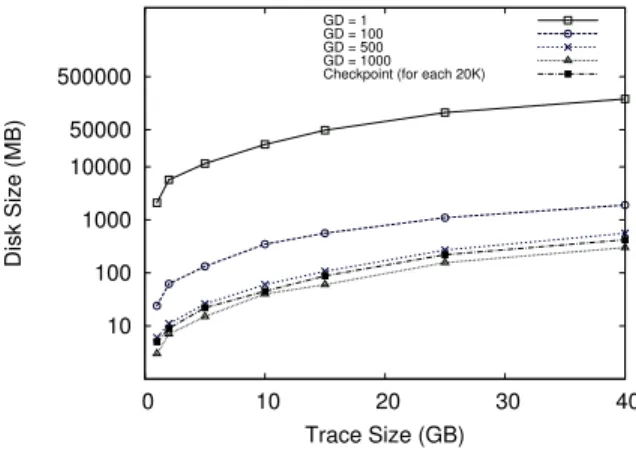
We have prototyped the proposed framework in Java on the Linux operating system. Linux kernel version 2.6.38.6 is in-strumented using LTTng, and the tests are performed on a 2.8 GHz machine with 6 GB RAM, using different trace sizes. This prototype will be contributed to TMF (Tracing and Mon-itoring Framework)5. In the prototype, the defined metrics are: CPU usage, IO throughout, number of network connec-tions (for both the incoming and outgoing HTTP, FTP, DNS connections), and also counts of different types of events. Figure 9 shows the memory used by the framework to store
10 100 1000 10000 50000 500000 0 10 20 30 40 Disk Size (MB) Trace Size (GB) GD = 1 GD = 100 GD = 500 GD = 1000 Checkpoint (for each 20K)
Fig. 9: Disk size of the interval tree data structure. the interval information. The graph shows different on-disk sizes for the different trace files. The trace files vary from 1 GB to 40 GB. The size of the resulting interval data store, where the granularity degree equals 1, is about 2.5 to 4.5 times the original trace size. As explained earlier, this is not a reasonable storage size. To solve this problem, larger granularity degrees (i.e. 100, 500, 1000) are used. Figure 9 depicts a comparison of the proposed method and the check-point method. Since the range of values for the case where the granularity degree is 1 is much higher than those with larger granularity degrees, the logarithmic scale is used for the Y axis.
A comparison of the tree construction time analysis be-tween different solutions (i.e. the checkpoint method, the his-tory tree, and the proposed method) is shown in Figure 10. The figure shows that the time used for tree construction con-siderably depends on the number of updates to the interval data store, and that the time decreases when less information is written to disk, thus underlining the importance of selecting coarse granularity degrees.
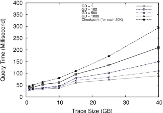
The query time analysis is shown in Figure 11. For each graph, we have tested 20 runs, in which we have used the aforementioned complete interval query (two stabbing queries for each request) for 100 randomly selected time intervals. As
0 1000 2000 3000 4000 5000 6000 7000 0 10 20 30 40
Construction Time (Second)
Trace Size (GB)
GD = 1 GD = 100 GD = 500 GD = 1000 Checkpoint (for each 20K)
Fig. 10: Construction time for different trace sizes.
0 50 100 150 200 250 300 350 400 0 10 20 30 40
Query Time (Millisecond)
Trace Size (GB)
GD = 1 GD = 100 GD = 500 GD = 1000 Checkpoint (for each 20K)
Fig. 11: Query time for different trace sizes.
shown in Figure 11, the best case is the tree with a granular-ity degree of 1000. In this case (and the cases with a gran-ularity degree of larger than 1), we have used linear interpo-lation to approximate the real values when querying a time within a checkpoint duration. With the checkpoint method, we reread the trace and regenerate the values inside the check-points. Since this method reopens and rereads the trace for each query, the query time is longer.
A comparison of the two aforementioned approaches for performing the hierarchical operations is shown in Figure 12. In this graph, the X axis shows the different points in the trace, and the Y axis shows the query time for computing the IO throughput of a process separately, a process and the whole system together using the first and second aforemen-tioned approaches. As explained earlier, computing the hier-archical statistics values, by summing up the containing val-ues, is faster than storing them separately in the interval tree, and querying them by reading the disk data structure for each query. As shown in the figure, summing up the values of containing resources in the busy areas of the system execu-tion (points 4,5) takes much more time than in the other trace
0 20 40 60 80 100 120 140 160 180 1 2 3 4 5 6
Query Time (Millisecond)
Different Trace Areas
Query timy for a single level query
Query timy by stroing the values of only the leaf nodes Query time by duplicating the values of all levels separately
Fig. 12: Comparison of different approaches for supporting the hierarchical operations.
points (points 1,2,6), in which the system is not too busy and encompasses less IO operations. The trace size 10 GB and granularity degree 100 are used for this comparison.
The analyzing of the above results shows that one can achieve better efficiency (both in disk size, construction time and query time) by using larger granularity degrees. However, this is not always true. The granularity degree is somehow re-lated to the precision of a metric. Larger degrees may lead to less precision, and longer query times for the points lying within an interval. Thus, a trade-off is required between the precision, granularity degree and the context of evaluation. However, more investigation is necessary to find proper val-ues for the granularity degrees of different metrics, as will be studied in a future work.
7. CONCLUSION AND FUTURE WORK Early steps in most analysis methods start by looking at the general overview of a given trace. The analysis can be con-tinued by narrowing the current view and digging into it to obtain more details and insight. The several previous studies that provide such a view are examined in the literature review. However, they are not able to compute system statistics in a relatively constant time for any given interval. We proposed a framework architecture to analyze large traces and generate and provide such a view. We also presented the performance results of this method.
The main effort was on creating a compact data structure that has reduced overhead, and a reasonable access and query time. The details of the proposed data structures and algo-rithms, with their subsequent evaluations for different cases have been analyzed. The framework models the system re-sources in a hierarchy to support hierarchical operations be-tween different resources. To avoid a size explosion of pre-computed statistics, a proper granularity degree should be cho-sen for each metric. Then, intermediate points are computed
using linear interpolation. Granularity can be expressed in count of events or time units. We evaluated the proposed framework by assigning different granularity degrees for dif-ferent metrics. The results denote that one can achieve a better efficiency and performance by determining proper granularity degrees for metrics. Constant access time (with respect to the time interval) for statistics computation is achieved by com-puting the final result from two values, at the start and end of the interval.
Possible future work is to analyze the effects of using the interpolation technique, as well as developing a formula to link the granularity degrees to metrics and trace sizes. We have prototyped the framework for LTTng Linux kernel tracer. Other future work includes extending the framework and re-lated data structures to support other tracing systems as well as connecting the proposed framework to kernel-based fault and attack detection systems.
Although the proposed method can be used for online tracing as well, this was not investigated during this phase of research. The online construction of the interval tree will probably lead to new challenges and will be experimented as a future work.
8. REFERENCES
[1] W. Fadel, “Techniques for the abstraction of system call traces,” Master’s thesis, Concordia University, 2010. [2] N. Ezzati-Jivan and M. R. Dagenais, “A stateful
approach to generate synthetic events from kernel traces,” Advances in Software Engineering, vol. 2012, April 2012.
[3] H. Waly, “A complete framework for kernel trace analysis,” Master’s thesis, Laval University, 2011. [4] M. Desnoyers and M. R. Dagenais, “The lttng tracer: A
low impact performance and behavior monitor for gnu/linux,” in OLS (Ottawa Linux Symposium) 2006, pp. 209–224, 2006.
[5] A. Shameli-Sendi, N. Ezzati-Jivan, M. Jabbarifar, and M. Dagenais, “Intrusion response systems: Survey and taxonomy,” SIGMOD Rec., vol. 12, pp. 1–14, January 2012.
[6] M. Bligh, M. Desnoyers, and R. Schultz, “Linux kernel debugging on google-sized clusters,” in OLS (Ottawa Linux Symposium) 2007, pp. 29–40, 2007.
[7] W. Xu, L. Huang, A. Fox, D. Patterson, and M. Jordan, “Online system problem detection by mining patterns of console logs,” in Proceedings of the 2009 Ninth IEEE International Conference on Data Mining, ICDM 09, (Washington, DC, USA), pp. 588–597, IEEE Computer Society, 2009.
[8] I. Cohen, S. Zhang, M. Goldszmidt, J. Symons, T. Kelly, and A. Fox, “Capturing, indexing, clustering, and retrieving system history,” SIGOPS Operating Systems Review, vol. 39, pp. 105–118, October 2005. [9] I. Cohen, M. Goldszmidt, T. Kelly, J. Symons, and J. S.
Chase, “Correlating instrumentation data to system states: a building block for automated diagnosis and control,” in Proceedings of the 6th conference on Symposium on Operating Systems Design Implementation -Volume 6, (Berkeley, CA, USA), pp. 16–16, USENIX Association, 2004.
[10] S. Kandula, R. Mahajan, P. Verkaik, S. Agarwal, J. Padhye, and P. Bahl, “Detailed diagnosis in enterprise networks,” SIGCOMM - Computer Communication Review, vol. 39, pp. 243–254, August 2009. [11] J. Desfossez, “Rsolution de problme par suivi de
mtriques dans les systmes virtualiss,” Master’s thesis, Ecole Polytechnique de Montreal, 2011.
[12] J. Srivastava and V. Y. Lum, “A tree based access method (tbsam) for fast processing of aggregate queries,” in Proceedings of the Fourth International Conference on Data Engineering, pp. 504–510, IEEE Computer Society, 1988.
[13] V. Gaede and O. Gunther, “Multidimensional access methods,” ACM Computing Surveys, vol. 30, pp. 170–231, June 1998.
[14] M. Renz, Enhanced Query Processing on Complex Spatial and Temporal Data. PhD thesis, 2006. [15] A. Montplaisir, “Stockage sur disque pour accs rapide
dattributs avec intervalles de temps,” Master’s thesis, Ecole polytechnique de Montreal, 2011.
[16] F. Giraldeau, J. Desfossez, D. Goulet, M. R. Dagenais, and M. Desnoyers, “Recovering system metrics from kernel trace,” in OLS (Ottawa Linux Symposium) 2011, pp. 109–116, June 2011.
[17] N. Sivakumar and S. S. Rajan, “Effectiveness of tracing in a multicore environment,” Master’s thesis,
Malardalen University, 2010.
[18] M. de Berg, O. Cheong, M. van Kreveld, and M. Overmars, Computational Geometry Algorithms and Applications 3rd edition. Springer-Verlag, 2008.