A conditionally heteroskedastic model
with time-varying coefficients for daily gas spot prices
Nazim Regnard and Jean-Michel Zakoïan
Les Cahiers de la Chaire / N°25
A conditionally heteroskedastic model with
time-varying coefficients for daily gas spot
prices
Nazim Regnard and Jean-Michel Zakoïan
a,b,c 1aCREST, Paris, France
bFIME, Paris, France
cEQUIPPE Université Lille 3, France
Abstract
A novel GARCH(1,1) model, with coefficients function of the realizations of an exogenous process, is considered for the volatility of daily gas prices. A distinctive feature of the model is that it produces non-stationary solutions. The probability properties, and the convergence and asymptotic normality of the Quasi-Maximum Likelihood Estimator (QMLE) have been derived by Regnard and Zakoian (2009). The prediction properties of the model are considered. We derive a strongly con-sistent estimator of the asymptotic variance of the QMLE. An application to daily gas spot prices from the Zeebruge market is presented. Apart from conditional het-eroskedasticity, an empirical finding is the existence of distinct volatility regimes depending on the temperature level.
Key words: GARCH, Nonstationary models, Periodic models, Quasi-maximum
likelihood estimation, Time-varying coefficients.
1 Introduction
Following the deregulation of natural gas markets in Europe, natural gas sup-plying historically ran by long term contracts indexed on crude oil between producing countries and retailers was diversified trough new financial markets (National Balancing Point in UK, Zeebrugge market in Belgium), where it
1 Corresponding author. CREST, 15, Boulevard G. Péri, 92245 Malakoff Cedex,
France. E-mail adress: [email protected]. Recherche réalisée avec le soutien de la chaire "Finance et développement durable".
can be freely sold at different time horizons. This restructuring has gener-ated uncertainty, requiring the development of appropriate valuation and risk management strategies.
Such strategies require an appropriate modeling of the prices volatility. The standard GARCH models of Engle (1982) and Bollerslev (1986), which ar-guably constitute the most important class of models for financial data may be inadequate for energy prices. The reason is that energy prices are subject to pronounced daily seasonal patterns, which may not only concern the condi-tional mean but also the volatility. The periodic ARCH model introduced by Bollerslev and Ghysels (1996) is able to capture those seasonal behaviors in the conditional variance. However, in this model the different regimes appear in a purely periodic succession and it may be worth introducing more flexibil-ity. A GARCH model with regression effects and scaled by seasonal factors has been recently proposed for electricity prices by Koopman, Ooms and Cornaro (2009).
The purpose of this article is to develop a new class of volatility models, introduced in a companion paper by Regnard and Zakoian (2009) (hereafter RZ), for characterizing the seasonal patterns induced by other variables such as temperature. In this model, the parameters associated with the volatility dynamics depend on an exogenous variable, similarly to papers dealing with the conditional mean by Azrak and Mélard (2006), Bibi and Francq (2003), Francq and Gautier (2004a, 2004b).
The article is organized as follows. Section 2 introduces the model and its main probability properties. It is shown how the model can be used for prediction purposes and the QML (Quasi-Maximum Likelihood) estimation is discussed. Section 3 proposes an application to gas prices. A preliminary treatment based on a vector error correction model, involving daily gas prices, brent prices and the temperature, is discussed. Finally, the proposed model is fitted with up to five volatility regimes depending on the temperature. The different spec-ifications are tested, and compared via out-of-sample predictions. Section 4 concludes. A technical proof is given in the appendix.
2 A nonstationary GARCH(1,1) model
The model we consider in this paper is given by
²t= σtηt, σ2t = ω(st) + α(st)²2t−1+ β(st)σ2t−1, t ∈ Z (1)
where (ηt) is a sequence of independent and identically distributed (iid),
values in a finite set E = {e1, . . . , ed}; the functions ω(·), α(·), β(·) are defined
on E with values in R+ with ω(·) > 0.
In our application, st will correspond to a level of temperature, observed at
time t. For each level of temperature, the volatility is that of a standard GARCH(1,1) model. Thus, if this level remains constant in some period, the volatility is governed by a standard GARCH. When another level of temper-ature is reached, the specification of the volatility changes. The existence of different regimes for the volatility, is a common feature between this model and the so-called Markov-switching GARCH models (see ...). However, the models interpretations are completely different. In Markov-switching models, the mechanism of regime change is governed by an non observable variable. In our model, it is governed by an observable process which is exogenous to the model. The dynamics of ²t is conditional to (St).
2.1 Probability properties
The probabilistic properties of this model have been established by Regnard and Zakoïan (2009). Assuming
A0: (st) is a realization of a process (St) which is stationary, ergodic, defined on
the same probability space (Ω, A, P) as (ηt), and independent of (ηt),
and letting
πj = P (St= ej), j = 1, . . . , d and a(x, y) = α(x)y2+ β(x),
RZ established that if γ0 := d X j=1 πjE{log a(ej, η0)} < 0, (2)
Model (1) admits a nonanticipative nonexplosive solution (²t). When γ0 > 0,
the process is explosive: for any initial value σ2
0, we have
In the ARCH(1) case (no coefficients β), Condition (2) takes the more explicit form Qd
j=1απj(j) < e−E log η
2
0. It can also be noted that the stability of the
GARCH(1,1) in each regime, that is
E{log α(j)η2
0 + β(j)} < 0, j = 1, . . . , d
is sufficient (but not necessary) for the global stability. A necessary condition for (2) is given by Qdj=1βπj(j) < 1.
Moreover γ1 := d Y j=1 {Ea(ej, η0)}πj < 1 ⇒ E²2t < ∞. (3)
2.2 Predictions of the squares
For standard GARCH(1,1) models, the optimal prediction of ²2
t in the L2
sense, E(²2
t | {²2t−`, ` > 0}), is obtained from the ARMA(1,1) representation
for the squares. Similarly, for Model (1), letting ut= ²2t − σt2 = (ηt2− 1)σt2 we
have
²2
t = ω(st) + (α + β)(st)²2t−1+ ut− β(st)ut−1.
Letting δt = ²2t − ω(st) − (α + β)(st)²2t−1, we thus have,
²2t= ω(st) + (α + β)(st)²2t−1−
X
k≥0
β(st) . . . β(st−k)δt−k−1+ ut. (4)
This representation is valid because (2) implies
d X j=1 πjlog β(ej) ≤ d X j=1 πjE{log a(ej, η0)} < 0,
from which the existence of the infinite sum in (4) is deduced, by the arguments used to establish the stationarity condition. Note that the expectation of ut
conditional on ²2
t past values is zero. The optimal predictor ˆ²2t of ²2t, in the L2
sense, is then
ˆ²2t = ω(st) + (α + β)(st)²2t−1−
X
k≥0
β(st) . . . β(st−k)δt−k−1.
Predictions at higher horizons can be derived similarly. Contrary to standard GARCH models, predictions formulas are time dependent trough the coeffi-cients st.
2.3 QML Estimation
The consistency and asymptotic normality of the QMLE have been proven under mild conditions by Berkes, Horváth and Kokoszka (2003) and Francq and Zakoïan (2004) for standard GARCH and ARMA-GARCH models. NZ showed that these properties can be extended to the model of this paper under assumptions which we now detail.
Let θ denote the vector of parameters,
θ = (ω(e1), . . . , ω(ed), α(e1), . . . , α(ed), β(e1), . . . , β(ed))0,
with true value θ0. The parameter is assumed to belong to a parameter space
Θ ⊂]0, +∞[d×[0, ∞[2d. The sequence (s
t) is observed, and the orders p, q and
d are known a priori. Let (²1, . . . , ²n) be a realization of length n of the
nonan-ticipative solution (²t). Conditionally on initial values ˜²0 and ˜σ02 the gaussian
quasi-likelihood is given by Ln(θ) = Ln(θ; ²1, . . . , ²n) = n Y t=1 1 q 2π˜σ2 t exp à − ² 2 t 2˜σ2 t ! , where the ˜σ2
t are defined recursively, for t ≥ 2, by
˜ σ2
t = ˜σ2t(θ) = ω(st) + α(st)²2t−1+ β(st)˜σ2t−1.
with ˜σ2
1 = ω(s1) + α(s1)˜²20 + β(s1)˜σ02. A QMLE (quasi-maximum likelihood
estimator) of θ is defined as any measurable solution ˆθn of
ˆ θn = arg max θ∈Θ Ln(θ) = arg minθ∈Θ˜ln(θ), (5) where ˜ln(θ) = n−1 n X t=1 ˜ `t, and ˜`t = ˜`t(θ) = ²2 t ˜ σ2 t + log ˜σ2 t.
Indexing the true parameter values by 0, we make the following assumptions.
A1: θ0 ∈ Θ and Θ is compact.
A2: Pd
j=1πjE{log a0(ej, η0)} < 0 and
Qd
j=1β πj
j < 1, where βj = supθ∈Θβ(ej).
A3: There exist r, ρ ∈ (0, 1) and C > 0 such that ∀i > 0, E {ar
0(St, ηt−1) . . . ar0(St−i, ηt−i−1)} < Cρi+1. (6)
A4: η2
t has a nondegenerate distribution with Eηt2 = 1.
A5: For all i, α0(ei) + β0(ei) 6= 0 and there exist ` ∈ {1, . . . , d} and k > 0
such that α0(e`)P(St−k = e`, St= ei) > 0.
A6: θ0 belongs to the interior of Θ.
A7: κη = Eηt4 < ∞.
Then, RZ showed that
(1) under A0-A5, almost surely θˆn→ θ0, as n → ∞,
(2) under A0-A7,√n(ˆθn−θ) is asymptotically N (0, (κη−1)J−1) distributed,
where J := ES,η Ã 1 σ4 S,t(θ0) ∂σ2 S,t(θ0) ∂θ ∂σ2 S,t(θ0) ∂θ0 ! (7)
is a positive-definite matrix, and (σ2
S,t(θ0)) is the process obtained by
replacing st by St in the second equation of (1).
The following examples illustrate the variability of the asymptotic covariance matrix, for given ARCH(1) coefficients with two regimes, depending on the distributions of (St) and (ηt). Let the model
²t= (1 + 0.1²2 t−1)1/2ηt if st = 1 (3 + 0.1²2 t−1)1/2ηt if st = 2 (8)
and suppose that (St) is a Markov chain with transition probabilities p(i, j).
Then, if • p(1, 1) = p(2, 2) = 0.5; ηt ∼ N (0, 1): Varas( √ n(ˆθn− θ)) = 7.41 0 −1.62 0 0 56.78 0 −8.96 −1.62 0 1.30 0 0 −8.96 0 5.28 ; • p(1, 1) = p(2, 2) = 0.95; ηt∼ N (0, 1): Varas( √ n(ˆθn− θ)) = 3.83 0 −1.33 0 0 300.51 0 −53.24 −1.33 0 1.58 0 0 −53.24 0 32.39 ;
• p(1, 1) = p(2, 2) = 0.95, ηt is distributed as a mixing og Gaussian
distribu-tions (with κη ≈ 9): Varas( √ n(ˆθn− θ)) = 11.39 0 −1.92 0 0 918.26 0 −77.02 −1.92 0 4.21 0 0 −77.02 0 87.99 ,
where these asymptotic covariance matrices have been obtained numerically, by simulation of Model (8). The presence of asymptotic covariances equal to zero for parameters of different regimes is due to the absence of coefficients β in the model.
2.4 Consistent estimation of the asymptotic variance of the QMLE
To build tests and confidence intervals for the parameters of Model (1), it is essential to have a consistent estimator of the asymptotic covariance ma-trix of the QMLE. In view of (7), this mama-trix depends on the distribution of (St) which is unknown. However, the following result provides a consistent
estimator which can be easily computed.
Proposition 1 Under Assumptions A0-A7, a strongly consistent estimator of the matrix J is given by
ˆ Jn= 1 n n X t=1 1 ˜ σ4 t(ˆθn) ∂ ˜σ2 t(ˆθn) ∂θ ∂ ˜σ2 t(ˆθn) ∂θ0 ,
and a strongly consistent estimator of (κη − 1)J−1 is
(ˆκη − 1) ˆJn−1, where κˆη = 1 n n X t=1 ²4 t ˜ σ(ˆθn)4 .
Proof. See appendix.
3 Application to gas prices volatility
We now turn to an example with real data, namely the daily series of gas spot prices from the Zeebruge market. Before modeling the volatility we filter the series from the conditional mean. To capture the joint behavior of the series of gas, Brent prices and temperatures, we consider a VAR model.
We have a sample of daily prices and temperatures from April, 5, 2000 through March, 3, 2008. Figure 1 displays a plot of the gas and Brent series, (Gt) and
(Bt) on the whole period. Let gt = log Gt and bt = log Bt denote the log
prices and let (Tt) denote the temperature series. Augmented Dickey-Fuller
and KPSS (Kwiatowski, Phillips, Schmidt and Shin, 1992) unit-root tests not reported here suggest that the series gt, bt and Tt are integrated of order one.
To filter the gas price conditional mean from the influence of the Brent oil price and the temperature, we use a vector error correction model (VECM). There is a growing literature examining the cointegration relationships between dif-ferent energy prices. Asche, Osmundsen, and Sandsmark (2006) discuss the cointegration between UK natural gas, Brent oil and electricity prices before and after the opening of the Interconnector in 1998. Bachmeier and Griffin (2006) found evidence of cointegration between crude oil, natural gas and coal
0.0 0.5 1.0 1.5 2.0 2000 2002 2004 2006 2008 10 20 30 40 50 2000 2002 2004 2006 2008
Fig. 1. Daily series of gas prices Gt (left panel) and Brent prices Bt (right panel).
in the USA. Panagiotidis and Rutledge (2007) found evidence of a cointegra-tion relacointegra-tionship between the UK wholesale gas prices and the Brent over the period 1996-2003, contradicting the assumption that gas prices and oil prices are decoupled since the liberalisation of gas markets in Europe.
3.1 A VECM for gas and brent prices
We begin the analysis with an error correction approach. Recall that, in Jo-hansen’s (1988, 1995) notation, a p-dimensional VECM takes the form
∆yt= k−1X
i=1
Γ∆yt−i+ Πyt−1+ µ + ut
where ∆ is the difference operator, yt is a p × 1 vector of I(1) variables, µ is a
drift parameter, (ut) is a white noise, Π = αβ0 is a p × p matrix where α and β
are p×r full-rank matrices, with β containing the r cointegrating vectors and α carrying the loadings in each of the r vectors. A preliminary analysis suggest that oil prices have an impact on gas prices with a delay of 13 weeks. Let yt = (gt, bt−τ, Tt) where τ = 91 days. The Johansen test rejects the null of zero
cointegrating vectors between the components of yt. The existence of r = 1
cointegrating relation is not rejected and the estimated cointegration vector is, by renormalizing so that the first element be unity, ˆβ = (1, −1.0809, 0.0194).
The estimated VECM is as follows. For ease of presentation, unsignificant coefficients, at the 5% level, have been omitted.
∆gt = −0.077 (gt− 1.080bt−τ + 0.019Tt+ 4.46) + 0.056 ∆gt−1 − 0.010 ∆Tt−4 (0.012) (0.030) (0.001) −0.103 ∆gt−5 − 0.091 ∆gt−6 − 0.087 ∆gt−8 − 0.003 ∆Tt−8 +²t (0.029) (0.029) (0.028) (0.001) ∆bt−τ = ζt ∆Tt = −0.218 ∆Tt−1 − 0.280 ∆Tt−2 − 0.225 ∆Tt−3 − 0.207 ∆Tt−4 (0.030) (0.031) (0.032) (0.032) −0.135 ∆Tt−5 − 0.107 ∆Tt−6 − 0.067 ∆Tt−8 + ξt (0.032) (0.032) (0.030)
It is worthnoting that for the brent prices, no significant linear influence of the past variables is detected. Results not reported here show that the process (²t, ζt, ξt) pass the diagnostic tests for the absence of autocorrelation.
3.2 Modelling the volatility of gas prices
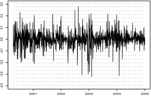
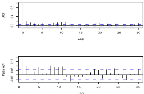
Figure 2 displays the series of residuals ²t for the gas prices. From Figure 3,
displaying the empirical autocorrelation function (ACF) and partial autocorre-lation function (PACF) of (²t), it is seen that this series has the characteristics
of a white noise. Caution is needed, however, in the interpretation of the sig-nificance bands under conditional heteroskedasticity (see Francq and Zakoian, 2009). The same graphs, displayed in Figure 4 for the series (²2
t), show that a
GARCH effect is present in the data.
The volatility models for the series ²twere estimated over the period april 2000
to december 2004, involving 1192 observations. To have a gauge, the following standard one-regime GARCH(1,1) model was fitted
σ2
t = 0.0003 + 0.13 ²2t−1 + 0.79 σt−12
(0.0000) (0.0006) (0.0011) (9)
where the standard errors appear in parenthesis. The GARCH coefficients are close to those generally obtained for financial series, with a strong persistence in volatility (α + β = 0.92).
Next, we turn to multi-regimes GARCH(1,1) models, where the regimes are determined by the temperature level. We start by a three-regimes model, where the three classes of temperatures correspond to approximately the same
num-−0.4 −0.3 −0.2 −0.1 0.0 0.1 0.2 0.3 Time 2001 2002 2003 2004 2005
Fig. 2. Series (²t) for the gas prices
0 5 10 15 20 25 30 0.0 0.4 0.8 Lag ACF 0 5 10 15 20 25 30 −0.06 0.00 0.04 Lag Partial ACF
Fig. 3. Empirical ACF and PACF of the series (²t). The bands ±1.96/√n are
dis-played in dotted lines.
ber of observations. This leads to choose st = 1 when Tt < 9, st = 2 when
Tt∈ [9, 14], and st= 3 when Tt > 14, with frequencies in the sample
0 5 10 15 20 25 30 0.0 0.4 0.8 Lag ACF 0 5 10 15 20 25 30 −0.05 0.05 0.15 Lag Partial ACF
Fig. 4. As in Figure 3 for the series (²2t).
The fitted three-regimes GARCH(1,1) model is as follows.
σ2 t = 0.0003 + 0.13 ²2 t−1 + 0.80 σt−12 when Tt < 9, (0.0002) (0.05) (0.06) 0.0011 + 0.37 ²2 t−1 + 0.36 σt−12 when 9 ≤ Tt≤ 14, (0.0004) (0.10) (0.16) 0.0004 + 0.14 ²2 t−1 + 0.76 σt−12 when Tt > 14. (0.0001) (0.06) (0.10) (11)
All coefficients, except the intercept in the first regime, are significant at the 5% level. The most striking point is the difference between the volatility dy-namics in the middle regime, compared to the volatilities of the two extreme regimes. The volatility of the second regime is less persistent (α(2) + β(2) = 0.73) with a more convex "news-impact curve". The impact of recent obser-vations on the volatility is stronger than in the low- and high-temperature regimes. It can be noted that the three GARCH(1,1) models are second-order stationary, which entails the global stability with a finite time-dependent variance for ²t. Note also that the marginal variances within each regimes
(ω(j)/(1 − α(j) − β(j)) are roughly the same (around 0.04).
The next model is based on a decomposition of the lower and upper regimes in (11). Letting st = 1 when Tt < 6, st = 2 when Tt ∈ [6, 9[, st = 3 when
frequencies are given by
π1 = 0.16, π2 = 0.19, π3 = 0.32, π4 = 0.15, π5 = 0.18. (12)
Using the estimated parameters of Model (11) as initial values in the numerical optimization routine, we get the fitted model
σt2 = 0.0008 + 0.15 ²2 t−1 + 0.80 σt−12 when Tt < 6, (0.0004) (0.08) (0.11) 0.0010 + 0.00 ²2 t−1 + 0.80 σt−12 when 6 ≤ Tt≤ 9, (0.0003) (0.04) (0.09) 0.0015 + 0.46 ²2 t−1 + 0.21 σt−12 when 9 < Tt≤ 14, (0.0004) (0.12) (0.17) 0.0007 + 0.32 ²2 t−1 + 0.62 σt−12 when 14 < Tt≤ 16, (0.0005) (0.12) (0.17) 0.0003 + 0.04 ²2 t−1 + 0.81 σt−12 when Tt > 16. (0.0003) (0.05) (0.13) (13)
The effects already noticed for the middle regime (little persistence and strong convexity of the news impact curve) is more pronounced with this five-regimes model. A strong coefficient α is also obtained in the fourth regime. On the contrary, the volatility in all other regimes mainly does not much depend on the last observation. Again, the model is globally stable in the second order sense.
The next model is aimed to detect the effect of extremely low or high tem-peratures. Letting st = 1 when Tt < 3.2, st = 2 when Tt ∈ [3.2, 9[, st = 3
when Tt ∈ [9, 14[, st = 4 when Tt∈ [14, 18.5[, and st = 5 when Tt> 18.5, the
regimes frequencies are given by
The fitted model is σt2 = 0.0036 + 0.38 ²2 t−1 + 0.47 σt−12 when Tt < 3.2, (0.0035) (0.35) (0.60) 0.0007 + 0.04 ²2 t−1 + 0.68 σt−12 when 3.2 ≤ Tt≤ 9, (0.0005) (0.07) (0.15) 0.0004 + 0.30 ²2 t−1 + 0.62 σt−12 when 9 < Tt≤ 14, (0.0005) (0.12) (0.18) 0.0004 + 0.20 ²2 t−1 + 0.72 σt−12 when 14 < Tt≤ 18.5, (0.0004) (0.10) (0.15) 0.0000 + 0.00 ²2 t−1 + 0.90 σt−12 when Tt > 18.5. (0.0070) (0.10) (0.43) (15)
However, many coefficients are found insignificant at the 5% level. Finally, we estimated a model in which the extreme temperatures (low and high) are gathered in the same regime. Letting st= 1 when Tt< 3.2 or Tt> 18.5, st= 2
when Tt ∈ [3.2, 9[, st = 3 when Tt ∈ [9, 14[, and st = 4 when Tt ∈ [14, 18.5[,
the regimes frequencies deduced from (14) are
π1 = 0.11, π2 = 0.29, π3 = 0.32, π4 = 0.28 (16)
and the estimated model is
σ2 t = 0.0026 + 0.34 ²2 t−1 + 0.41 σt−12 when Tt < 3.2 or Tt > 18.5, (0.0012) (0.13) (0.26) 0.0004 + 0.08 ²2 t−1 + 0.75 σt−12 when 3.2 ≤ Tt≤ 9, (0.0003) (0.05) (0.09) 0.0011 + 0.38 ²2 t−1 + 0.35 σt−12 when 9 < Tt≤ 14, (0.0004) (0.11) (0.18) 0.0004 + 0.08 ²2 t−1 + 0.75 σt−12 when 14 < Tt≤ 18.5. (0.0004) (0.07) (0.15) (17)
The likelihoods of the different models, displayed in Table 1 allow to compare the different fits. From likelihood ratio tests, at the 5% significance level, • the standard GARCH(1,1) model is not rejected against the 3 regimes
model;
• the GARCH(1,1) model is however rejected against any model with d > 3; • the 3 regimes model is rejected against the 5 regimes Model (13).
Wald tests not reported here lead to the same conclusions. In the same table, the estimated kurtosis of the variable ηt = ²t/σt are reported. The biggest
Table 1
Likelihoods of the estimated models and Kurtosis of the standardized returns GARCH Model (11) Model (13) Model (15) Model (17)
(d = 1) (d = 3) (d = 5) (d = 5) (d = 4) log Ln 5173 5179 5206 5210 5187
ˆ
κη 6.00 5.76 5.43 5.68 5.63
Table 2
MSE (×10−5) of predictions (last 500 observations)
GARCH Model (11) Model (13) Model (15) Model (17) (d = 1) (d = 3) (d = 5) (d = 5) (d = 4)
7.66 7.57 7.29 7.47 7.47
Table 2 reports Mean-Squared Errors (MSE) of prediction. We re-estimated the different models over the same sample minus the last 500 observations, which were used for the predictions. The estimated models over the sample were very close to those estimated on the whole sample. From the prediction point of view, the 5-regime Model (13) is again the preferred specification.
4 Conclusion
This paper reviewed a class GARCH models, which allow the volatility to depend on an observed exogenous process. This observability of the state vari-able makes the model much easier to use than the so-called Markov-switching models in which the regime change is governed by a latent Markov chain. The model can be estimated by QML and a consistent estimator of the asymptotic covariance matrix has been proposed. The methodology has been applied to daily gas prices using the temperature as the exogenous variable. We found evidence of five regimes, with very different dynamics for the volatility in the moderate-temperature regime. The model could be used for prediction pur-poses, using temperature scenarios. Many extensions, by including more lags in the volatility dynamics or by considering multivariate series, are left for future research. It is hoped that the article will broaden the use of time series models driven by exogenous variables.
A Technical details
Proof of Proposition 1. For all θ ∈ Θ, let
˜ Jn(θ) = 1 n n X t=1 1 ˜ σ4 t(θ) ∂ ˜σ2 t(θ) ∂θ ∂ ˜σ2 t(θ) ∂θ0 , Jn(θ) = 1 n n X t=1 1 σ4 t(θ) ∂σ2 t(θ) ∂θ ∂σ2 t(θ) ∂θ0 .
Note that ˆJn= ˜Jn(ˆθn). We have, letting θ = (θi)i=1,...,3d,
1 n n X t=1 ( 1 σ4 t ∂σ2 t ∂θi ∂σ2 t ∂θj ) θ=ˆθn =1 n n X t=1 ( 1 σ4 t ∂σ2 t ∂θi ∂σ2 t ∂θj ) θ=θ0 + 1 n n X t=1 ( ∂ ∂θ0 Ã 1 σ4 t ∂σ2 t ∂θi ∂σ2 t ∂θj !) θ=θ∗ ij (ˆθn− θ0). (A.1) where θ∗
ij is between ˆθn and θ0. Denote by (σ2S,t(θ)) the process recursively
defined under A2 by σ2
S,t(θ) = ω(St) + α(St)²2t−1+ β(St)σS,t−12 (θ). We have,
for almost all sequence (st),
lim sup n→∞ ° ° ° ° °n −1Xn t=1 ∂ ∂θ0 Ã 1 σ4 t(θij∗) ∂σ2 t(θij∗) ∂θi ∂σ2 t(θ∗ij) ∂θj !° ° ° ° ° ≤ lim sup n→∞ n −1Xn t=1 sup θ∈V(θ0) ° ° ° ° ° ∂ ∂θ0 Ã 1 σ4 t(θ) ∂σ2 t(θ) ∂θi ∂σ2 t(θ) ∂θj !° ° ° ° ° = Eθ0 sup θ∈V(θ0) ° ° ° ° ° ∂ ∂θ0 Ã 1 σ4 S,t(θ) ∂σ2 S,t(θ) ∂θi ∂σ2 S,t(θ) ∂θj !° ° ° ° °< ∞.
where k · k denotes any norm on R3d. The equality follows from Lemma
5.2 in RZ and the fact that σ2
t(θ) and ∂σ2
t(θ)
∂θ are measurable functions of
(st, st−1, . . . , ηt, ηt−1, . . .). The last inequality is a consequence of iii), in the
proof of Theorem 4.2 in RZ. Since ˆθn − θ0 → 0 a.s., the last term in (A.1)
converges to zero in probability as n tends to infinity.
Using again Lemma 5.2 in RZ, we obtain the a.s. convergence to J of the first term in the right-hand side of (A.1). Thus we have shown that
1 n n X t=1 ( 1 σ4 t ∂σ2 t ∂θi ∂σ2 t ∂θj ) θ=ˆθn → J, a.s. Since, by FZ, Proof of Theorem 4.2,
sup θ∈V(θ0) ° ° ° ° ° 1 n n X t=1 ( ∂2`˜ t(θ) ∂θ∂θ0 − ∂2l t(θ) ∂θ∂θ0 )° ° ° ° °→ 0 a.s.
where `t(θ) is defined as ˜`t(θ) with ˜σt replaced by σt, we thus have ˆ Jn = 1 n n X t=1 ( 1 ˜ σ4 t ∂ ˜σ2 t ∂θi ∂ ˜σ2 t ∂θj ) θ=ˆθn → J, a.s. By the same arguments we prove that
ˆ κη = 1 n n X t=1 ²4 t ˜ σ(ˆθn)4 → Eη4 t
and the proposition is proved.
References
Asche, F., Osmundsen, P., Sandsmark, M., 2006. The UK market for natural gas, oil and electricity: Are the prices decoupled? Energy Journal, 27, No.2, 27–40.
Azrak, R., Mélard, G., 2006. Asymptotic properties of quasi-maximum likeli-hood estimators for ARMA models with time-dependent coefficients. Sta-tistical Inference for Stochastic Processes 3, 279-330.
Bachmeier, L.J., Griffin, J.M., 2006. Testing for market integration : crude oil, coal, and natural gas. The Energy Journal 27, 55–71.
Berkes, I., Horváth, L., Kokoszka, P., 2003. GARCH processes: structure and estimation. Bernoulli 9, 201–227.
Bibi, A., Francq C., 2003. Consistent and asymptotically normal estimators for time-dependent linear models. Annals of the Institute of Statistical Mathematics, 55, 41–68.
Bollerslev, T., 1986. Generalized autoregressive conditional heteroskedasticity. Journal of Econometrics 31, 307–327.
Bollerslev, T., Ghysels, E., 1996. Periodic autoregressive conditional het-eroskedasticity. Journal of Business and Economic Statistics 14, 139–151. Cai, J., 1994. A Markov model of switching-regime ARCH. Journal of Business
& Economic Statistics 12, 309–316.
Engle, R.F., 1982. Autoregressive conditional heteroskedasticity with esti-mates of the variance of the United Kingdom inflation. Econometrica 50, 987–1007.
Fong, P.W., Li, W.K., An, H.Z., 2006. A simple multivariate ARCH model specified by random coefficients Computational Statistics & Data Analysis 51, 1779–1802.
Francq, C., Gautier, A., 2004a. Large sample properties of parameter least squares estimates for time-varying ARMA models. Journal of Time Series Analysis 25, 765-783.
with Markovian changes in regime. Statistics and Probability Letters 70, 243-251.
Francq, C., Zakoïan, J-M. 2004 Maximum likelihood estimation of pure GARCH and ARMA-GARCH processes. Bernoulli 10, 605-637.
Francq, C. and Zakoïan, J-M. 2009. Bartlett’s formula for a general class of non linear processes. Journal of Time Series Analysis, 30, 449–465.
Gray, S.F., 1996. Modeling the conditional distribution of interest rates as a regime-switching process. Journal of Financial Economics 42, 27–62. Hamilton, J.D., 1989. A new approach to the economic analysis of
nonstation-ary time series and the business cycle. Econometrica 57, 357–384.
Hamilton, J.D., Susmel, R., 1994. Autoregressive conditional heteroskedastic-ity and changes in regime. Journal of Econometrics 64, 307–333.
Johansen, S., 1988. Statistical analysis of cointegration vectors. Journal of Economic Dynamics and Control 12, 231–254.
Johansen, S., 1995. Likelihood-based inferencein cointegrated vector autore-gressive models. Oxford University Press, Oxford.
Koopman, S.J., Ooms, M., Carnero, M.A., 2007. Periodic Seasonal Reg-ARFIMA-GARCH Models for Daily Electricity Spot Prices. Journal of the American Statistical Association 102, 16-27.
Kwiatowski, D., Phillips, P.C.B., Schmidt, P., and Shin, Y., 1992. Testing the null hypothesis of stationarity against the alternative of of a unit root: how sure are we that economic time series have a unit root? Journal of Econometrics, 54, 159–178.
Panagiotidis, T., Rutledge, E., 2007. Oil and gas markets in the UK: Evidence from a cointegrating approach. Energy Economics 29, 329–347
Regnard, N., Zakoian, J-M. 2009. Structure and estimation of a class of nonstationary yet nonexplosive GARCH models. Dis-cussion paper, Laboratoire FIME. Available at http://www.fime-lab.org/fr/index.php?section=publications.