Health, Pension Benefits and Longevity How They Affect Household Savings?

Najat El-Mekkaoui de Freitas and Joaquim Oliveira

Martins

Health, Pension Benefits and

Longevity

HEALTH, PENSION BENEFITS AND LONGEVITY: HOW THEY AFFECT HOUSEHOLD SAVINGS?

Najat El-Mekkaoui de Freitas and Joaquim Oliveira Martins*

Abstract

This paper analyses the impact of health, pension systems and longevity on savings. It uses a simple life-cycle model embodying social transfers (health care and pension expenditures) and changes in longevity to determine the level of household savings. From this model, we derived an econometric specification, augmented with the effects of public budget balances. The model is estimated for a panel of 22 OECD countries for the period 1970-2009. Our principal result is that, from the point of view of incentive to save, health transfers have a similar impact as pension replacement rates. Therefore, welfare reforms that reduce replacement rates without reforming health system may not have all the expected impact on household savings. In line with life-cycle theory, we found that longevity increases saving ratios.

JEL Classification: D91, I13, J1, J11, J26

Key words: Ageing, Consumption, Health, Longevity, Pension systems, Saving

October 2013

(*) El-Mekkaoui de Freitas: PSL Université Paris-Dauphine LEDA-DIAL and NETSPAR, email: najat.el-mekkaoui@dauphine.fr; Joaquim Oliveira Martins: OECD and PSL, Université Paris-Dauphine, email: joaquim.oliveira@oecd.org. The authors thank Hippolyte d’Albis, Johannes Clemens, Carlo Cottarelli and Christophe Hurlin and for helpful discussions. Christine de la Maisonneuve provided helpful technical support. El-Mekkaoui de Freitas is grateful to the “Chaire Dauphine-Ensae Groupama” for their support. The views expressed are those of the authors and

1. Introduction

The life cycle hypothesis is the main framework used in economics to model the relations between age, consumption and saving behaviour. It has been largely used to understand households’ saving behaviour, design pension reforms and manage the effects of ageing. In this context, the main focus of this paper is to understand the impact of pension and public health systems on household saving behaviour. In this paper we use a life-cycle model combining the impact of pension replacement rates, together with provision of public health care and longevity on savings. On its basis, we then develop a reduced-form estimated through a panel data set including 22 OECD countries from the period 1970-2009.

Our approach relies on a number of previous papers, which aimed to reconcile observed saving behaviour facts with the life-cycle theory. Concerning the impact of welfare systems, our starting point is the seminal paper by Feldstein (1974) who highlighted a negative link between Pay-As-You-Go (PAYG) pension systems and household savings. Subsequent empirical tests on the impact of pension systems on household saving have produced mixed results (e.g. Edwards, 1996; Baillu and Reisen, 1997; Callen and Thimann, 1997; Corsetti, Schmidt-Hebbel, 1995, Bosworth and Burtless, 2004; and Murphy and Musalem, 2004). Sample heterogeneity, however, has made these results difficult to compare.1 The empirical results presented in this paper would tend to endorse the view that welfare systems may generate disincentives to save.

Concerning the impact of longevity, Bloom et al. (2003) argued that higher life expectancy should lead to an increase of precautionary savings. Empirical work, however, has also found an opposite sign. More recently, Bloom et al. (2006) have shown that in the absence of strong saving retirement incentives, such as in PAYG systems, an increase in longevity does not induce higher savings.2 This remains an empirical issue to be addressed. Our results support a positive link between longevity and savings.

The impact of health consumption on savings can be related, among others, to an observed fall in consumption in other consumption goods after retirement. This is a stylized fact observed in most OECD countries (e.g. US, UK and Italy), across time periods and for different measures of household spending. It seems to contradict the hypothesis that marginal utility of consumption should be the same before and after retirement. A possible explanation would be to assume that retirement may occur as the result of an anticipated shock. This uncertainty could generate a fall in consumption at retirement,3 but the estimated impact of this effect is small (see Blau, 2008). Thus,

1. Edwards (1996) found that the social security system has a negative impact on private saving using a sample of 32 countries (developed and developing countries). Baillu and Reisen (1997) also found a positive and statistically significant impact of pension funds on savings using a panel of 11 countries for the period 1982-93. On the other hand, Bosworth and Burtless (2004) did not find any econometrically significant impact on private saving for a set of 11 countries during the period 1971-2000. Murphy and Musalem (2004) considered 43 countries for the period 1960-2002 and found that only mandatory contribution to funded pension systems increase national saving.

2. This of course only holds when the age of retirement is fixed and not linked to longevity, which is still the case in most social security systems in OECD countries.

other explanations should be considered. Accordingly, some authors (e.g. Browning and Lusardi, 1996; Browning and Crossley, 2001) suggest that a deterioration of health status, a decrease of family size or increased mortality risk could reduce the marginal utility of consumption. Allowing for uncertainty, Banks, Blundell and Tanner (1998) argued that unanticipated shocks occurring around the date of retirement could explain the fall in spending within the context of the life-cycle model, while Bernheim, Skinner and Weinberg (2001) argued that workers do not adequately foresee the decline in income associated with the retirement or the risks associated with different retirement saving and pension schemes (Clark and Strauss, 2008).

Aguiar and Hurst (2005, 2009) argued that when non-durable expenditures are disaggregated into detailed consumption categories, work-related expenditures account for most of the decrease in consumption. Along these lines, Hurd and Rohwedder (2003) suggested that the drop in consumption spending cannot be explained by the simple one-good life cycle model, with forward-looking consumers. Certain work-related consumption expenditures stop at retirement and market-purchased goods and services are substituted by household home production. Notably, long-term care services are often provided informally within families.

We follow the latter argument and consider in our model that a different basket of goods is consumed in active life and retirement, in particular the share of health consumption is typically higher after retirement.4 This approach has been pursued in a number of papers analysing the impact on ageing on health and productivity (e.g. Aisa and Pueyo, 2013) in a general equilibrium context. In this paper we rather focus on the impact of welfare systems and argue that the fact that the bundle of consumption at old-age could be twisted towards a heavily subsidised good, such as health care, might decrease savings. To model this less-explored relationship among saving determinants, we use a two-period optimal consumption model, with social welfare transfers and longevity. We use this framework to derived a reduced-form also controlling for other traditional determinants of savings, such as the Ricardian compensation between private and public savings.

The next section motivates the research by describing key empirical facts on age, consumption and welfare goods. Section 3 presents the life-cycle model used in this paper. In section 4, presents econometric panel estimates. A final section concludes.

2. Stylised facts on age, consumption and welfare goods

It is well-known that total consumption displays a hump-shaped profile across age-groups. More precisely, the consumption profile is hump-shaped across households headed by individuals belonging to different age groups. This is not equivalent to say that the consumption profile is hump-shaped over the life cycle mainly due to the possible existence of cohort and time effects. Nonetheless, Fernandez-Villaverde and Krueger (2007) suggest that the bias induced by the use of age-groups instead of cohorts may not be very large for the estimation of the hump-shaped consumption profiles. Therefore, the snapshot picture of total consumption per household by age-groups can approximate the life-time consumption profile of a cohort (e.g. static ageing as opposed to dynamic ageing). This approach takes an agnostic view on how a combination of various

4. Note that age by itself is not a major driver of health care expenditures, but other factors such as the proximity to death, the effects of income and technological progress. In contrast, the expenditures of long-term care are mainly determined by the age profile (see Oliveira Martins and de la Maisonneuve, 2006 for a discussion).

household characteristics in conjunction with institutional factors in each country affects the life-cycle consumption pattern. Note that when the age-income profile is more hump-shaped than consumption, the above observed age-consumption patterns are still compatible with some consumption smoothing over the life cycle (Attanasio, 1999). Most expenditure items also display a hump-shaped profile, with consumption level per capita increasing steadily with age, peaking at middle-age then decreasing. However, health care is one the few consumption items that tends to increase with age.

Health care is also heavily subsidised in most countries. The shares of publicly provided health services to household income increased steadily since the 1970s (e.g. in France, Sweden, UK and USA, see Figure 1). By 2003, the ratios of public health expenditures to Household income ranged from 5-7% in UK and US to 10-15% in France and Sweden.

[Figure 1. Ratio of Public Health Expenditure to Household income]

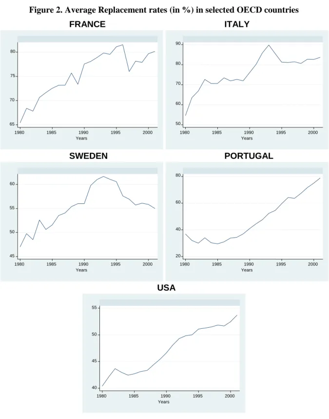
At the same time, average replacement rates also increased in most countries (Figure 2).5 For example, in France, Italy and Portugal they had reached close or above 80% by 2003. In US, starting from a lower basis they reached nearly 55%. Only in Sweden they have declined to around 55% following pension reforms.

[Figure 2. Average replacement rates in OECD countries] 3. The impact of welfare systems and longevity on savings

The most widely used framework to study the link between ageing, consumption and saving is the life cycle model (Modigliani and Brumberg, 1954; Ando and Modigliani, 1963; Friedman, 1957). In its simplest version, individuals live two periods. In the first period each person earns a wage from his/her labour supply and, in the second period, the person retires. Individuals save from their wage income to provide for the second-period consumption with a constant rate of interest (i.e., the rate of interest does not vary with the level of saving). The main result obtained from this framework is that the consumption is smoothed in the sense of holding marginal utility constant during the life: the individuals will save in order to transfer purchasing power to the period of the retirement.

To guide our investigation of the ageing-related facts described above, we use a simple life-cycle model. Following Yaari (1965), Bohn (1999) and Chakraborty (2004), we consider a two-period overlapping generation’s model (hereafter, OLG) with a survival probability.6

This provides a tractable framework to think about the different determinants of savings at the individual level. Our aim is to consider the institutional settings of the welfare system after retirement and how they impact saving behaviour. The model combines Pay-as-You-Go (PAYG), funded pension retirement incomes and welfare transfers (e.g. public health insurance). Each agent optimises her/his consumption and saving over the two periods. In the first period, each agent splits disposable wages

wi into a bundle of consumption goods (Ci) and saving (Si):

5. Average replacement rates are defined here as the ratio between average pension benefits to gross average wages. They were computed using the data OECD Pension and ADB databases.

6. In another context, Jorgensen and Jensen (2008) incorporate the survival probability in a stochastic OLG model with endogenous labour supply.

i i

i S w

C  (1). (1)

Where α is the rate of social contributions.

Following Hurd and Rohwedder (2003), we consider two different bundles of goods in active life and retirement. This captures the change in the structure of consumption. In the bundle of goods (Hi)7 consumed in the second period certain goods such as health and long-term care would have a

much stronger weight and could be highly subsidised.

To finance consumption in the second period, the agent receives a PAYG pension with a replacement rate β, the accumulated saving accrued by the return on capital r and a given amount of transfers (T) subsidising health consumption. Note that the amount of savings accumulated for the second period has to be scaled down by the survival probability pi (assumed to be strictly positive)

given that when the latter increases, the consumption has to be spread over a longer retirement period, as follows:8 0 with ) 1 ( .       i i i i i i S T p p r w H  (2)

Note that this introduces uncertainty not on the age of retirement, but on its duration. This enables to focus on longevity effects and is a departure from standard two-period OLG models. By definition, the income from the PAYG system and the welfare transfers are not affected by changes in the longevity (at least at the individual level). Also note that we did not introduce a pure time-preference parameter because, under uncertainty, the survival probability captures the effect of the discounting parameter (see Chakraborty, 2004).9 To simplify, we omitted the index corresponding to the time period.

Solving for Si in (2) and replacing into (1), we obtain the inter-temporal budget constraint:

) ( 1 1 ) 1 ( 1 i i i i i i i i w r p T r p w H r p C                (3)

Maximising the utility of each agent under the budget constraint (3), we obtain:









7. This assumption does not entail a loss of generality in the model, as we could have introduced a composite consumption good in the form δ.C + (1- δ).H, with the weight δ changing from period 1 to period 2.

8. Using a survival probability is identical to modelling the length of life in the retirement period. Note that this probability is an indication of life expectancy. By normalising the duration of one period to one, life expectancy is by definition (1+p). For example, if period 1 is equal to 60 years and total life expectancy is 84, the survival probability in this context is (24/60)=0.4.

First-order conditions imply that: ) 1 /( ) ( ) ( r H u C u i i i i        (5)

Where λi is the Lagrange multiplier associated with the budget constraint. Using these conditions we

obtain the usual consumption-smoothing rule: ) 1 ( ) ( ) ( r H u C u i i     (6)

As in Bohn (1999) and Chakraborty (2004), we assume thereafter that the u(C) = Log(C) and idem for H.10 We then get a simple relation between Ci and Hi:

i

i r C

H (1 ) (7)

Now replacing (7) into the budget constraint:

) ( 1 1 ) 1 ( i _i i i i i i i w r p T r p w C p C               (8)

The optimal level of consumption in each period can be derived:





By using the expression for the optimal consumption above and equation (1), we derive the optimal gross saving rate in the first period:

              ) 1 ( / ) 1 ( 1 r w T p p w S s i i i i i i i   (10)

Depending on the values of the different parameters, the expression above in square brackets can be negative, which also implies negative individual savings. This can only occur for very high values of replacement rates. For example, assuming welfare transfers at 10% of the wage income, a contribution rate of 20% and an interest rate at 3%, when replacement rates are above 72% individual savings become negative.11 Even this may be seen as an extreme case, in several OECD

10. A log-utility implies homothetic preferences. Nonetheless, the main results of the model used in this paper derive from the existence of the conditional life expectancy and from the intertemporal budget constraint. 11. In the case where there is no perfect consumption smoothing, an increase of the replacement income could

countries replacement rates had increased steadily over the past decades (Figure 4, above) inducing strong disincentives for savings.

The derivative of the optimal saving ratio (s) vis-à-vis the survival probability also depends from the same expression involving the parameters of the welfare system:

i i i i i i i w T r if r w T p p s _{     }                      ) 1 ( ) 1 ( 0 ) 1 ( / ) 1 ( 1 1 2 _  _{ } (11)

For small values of the replacement rate (β), an increase of the survival probability increases the saving ratio. In other words, a person experiencing a higher longevity has to save more to ensure an adequate consumption level during a longer retirement period. For larger values of the replacement rate, the sign of the derivative can be reversed, but from (10) this also corresponds to the existence of negative savings, which is rather unlikely for a large sample of countries.

To some extent, variation in the welfare transfer ratio (Ti/wi) also induces a change in the sign

of s_i p_i, but this would happen only for very large values of β. Under the still high replacement rates prevailing in many OECD countries, our model can therefore provide an explanation for weak or negative effects of longevity on household saving. In other words, the so-called ‘longevity puzzle’ is actually not be in contradiction with life-cycle theory.

The derivatives of the saving ratio (s) vis-à-vis the other key parameters in the model are defined in a non-ambiguous way, as follows:

0 and 0 ; 0 ; 0 ; 0               si  si Ti si i si r si wi (12)

The saving rate is expected to be a decreasing function of the replacement ratio, welfare transfers to older people and the rate of social contributions (α). In other words, the systems providing large transfers and generous retirement income (typically PAYG) are expected to have ceteris paribus lower individual saving rates. Conversely, the saving ratio depends positively from income and the interest rate.

Assuming that all individuals are identical in each period, the social budget constraint associated with the equilibrium of the social welfare system can be written as follows:









Where NY is the total number of young (active) population and NO is the number of retired people.

Total population is N=NY+NO. From (13) one can derive the endogenous parameters ensuring the

equilibrium of the welfare system in each period. The contribution rate satisfying the social budget constraint (~) is:

i T T w w w T N N i i Y O                 

 assumingthat and

~ _

 (14)

As it could be expected, the rate increases with the old-age dependency ratio (NO/NY). Following

pension reforms, the system can also be adjusted through the replacement rate:

w T N N_{O Y}    ~ (15)

The replacement rate respecting the social budget constraint (~) decreases as the old-age dependency ratio increases. Another adjustment variable could be the welfare transfer T (subsidising health consumption). It is likely that in the long-run the sustainability of welfare systems would entail a combination of these adjustment factors (α, β or T).

In order to derive the aggregate saving rate respecting the social budget constraint, we have to sum individual savings and adopt a sustainability rule for the welfare system. If we assume that the system is balanced through the contribution rates, parameter (α) in equation (10) should be replaced by (~) from equation (14). Given that savings in the second period are by definition zero, after some algebra we obtain an aggregate gross saving ratio:

i p p r N N w T p p w S i Y O N i i N i i y y                             





As suggested by life-cycle theory, the aggregate saving ratio is expected to be negatively related to the old-age dependency ratio.

As such equation (16) is an identity providing guidance on potential determinants of savings, but cannot be estimated parametrically. Moreover, it does not capture all the factors influencing savings. Therefore, the empirical test will have to rely on a reduced form and control for other determinants explaining household saving behaviour. A possible effect is the compensation between private and public savings or the, so-called, Ricardian equivalence (Barro, 1974). When government budgets (hereafter, BAL) are running on debt or public pension systems are not sustainable, households anticipate a required increase in future taxes and/or lower transfers and adjust upwards their savings. For a large panel of OECD countries, we observe indeed that the level of household savings is inversely correlated with the level of public deficits (Figure 3). This effect will be introduced in the econometric specification discussed below.

[Figure 3. Public budget balances and Household saving rates]

Another determinant not captured in our simple theoretical model, is the possibility for households to have positive savings after retirement. As suggested in the literature reviewed above, this could be due to habit persistence and/or deterioration in health conditions, making elderly people less able to spend as much as they would like to do. These excess savings are particularly observed under

welfare systems with high pension replacement rates and health care provision (cf. Börsch-Supan et

al., 2000, 2003).

Other explanations have been found in the literature using microdata. For American households, Scholz et al. (2004) note that tax incentives, as IRAs and 401(k), may lead to excess savings. A largely evoked reason for saving at older ages has been the existence of bequests, but excess savings due to these motives seem limited (Caroll, 2000). In a recent paper, De Nardi et al. (2010) show that the risk of living longer increases uncertainty related to expensive medical care and income effects are significant. Both explain why the elderly could save after retirement.

To consider these facts and allow for both old-age replacement rates and public Health expenditures to have an impact on excess savings, we will include in the econometric specification two interaction terms: i) between the replacement rates and the old-age dependency ratio; ii) between the public Health expenditures and the old-age dependency ratio. They may capture a possible reversal on the sign of high replacement rates and public health expenditures on savings after retirement.

4. Econometric estimates combining the different determinants of savings

The structural model (16) suggests a functional form for the determinants of savings, with expected signs as follows:













The determinants of this structural model and the additional explanatory variables discussed above are then combined in a linear reduced-form equation.

This flexible specification accounts for a variety of saving determinants identified in the literature (e.g. Edwards, 1996; Loayza, Schmidt-Hebbel and Serven, 2000; Börsch-Supan and Lusardi, 2003, Murphy and Musalem 2004). More precisely, the empirical model is specified as follows:

t i t i t i t i t i t i t i t i t i t i t i t i t i TREND BAL r Olddep TH Olddep RR Olddep TH RR LE Y S , 9 , 8 , 7 , , 6 , , 5 , 4 , 3 , 2 , 1 0 , , _ _ 60                       (18)

The variables and parameters entering in the equation are derived from different data sources:

S/Y: the ratio of household saving to income is our dependent variable.12 To be coherent with the equation (16), this ratio should only include the saving and revenues from active population.

12. Household saving is defined here as household disposable income less consumption. Household income consists primarily of the compensation of employees, self-employment income, and transfers. Property and other income - essentially dividends and interest - are evaluated in the light of business income and debt interest flows. The sum of these elements is adjusted for direct taxes and transfers paid to give household disposable income. Note that SNA93/ESA95 has changed the concept of disposable income for households (compared with SNA68/ESA79) so as to include private pension benefits and subtract private pension contributions.

Given that these data are not available, we simulated a gross household saving ratio vis-à-vis both household income.13 All these variables were extracted from the OECD ADB Database.

LE60: As noted above, in the context of our two-period life-cycle model, the survival probability

can be defined as the ratio of the numbers of years in retirement (period 2) to the numbers of years in active life (period 1). If we take the age of retirement at 60, then the term p/(1+p) in equation (16) is equal to ratio of life expectancy at 60 divided by the life expectancy at birth. These variables were derived from the OECD Population database.

RR: The average gross replacement rate was calculated as the ratio between the average pension

revenues to average wages, derived both from the OECD ADB and Pension Databases (cf. OECD, 2011, page 118). This proxy is the only available for a large sample of countries and years.14

TH: is estimated by the ratio of Public health expenditures to GDP. The health expenditures were

obtained from the OECD Health database.

Olddep: is the old-age dependency ratio computed as old-age (60+) population divided by the

population aged (25-59). Population data are derived from national statistical offices gathered in the OECD Population database.

RR_Olddep: interaction term between the replacement rate and the old-age dependency ratio. TH_Olddep: interaction term between the Public health expenditures to GDP ratio and the

old-age dependency ratio.

r is the long-term real (representative) interest rate derived from the OECD ADB database. BAL: Public budget balance (in % GDP) derived from OECD ADB Database.

TREND: is a time trend common to all countries.

ε is a normally distributed error term. A time trend was also introduced as an additional control for

an eventual drift in the household saving rates.

The model was estimated in a unbalanced panel of 22 OECD countries,15 for which the data were the most complete over the period 1970-2009. Annex 1 provides descriptive statistics on the different variables used in the regressions. To test for the robustness of the coefficients, we first estimated the pooled model, then country fixed-effects with and without a time dummies (replacing the time trend). Furthermore, we tested additional specifications using the random-effects and the dynamic panel estimator of Arellano-Bond (1991). In our case however, the random-effect specification cannot be accepted on basis of the Hausman test (cf. Table 1).

13. The ratio to household income is in principle the best measure, although a potential problem is that it also includes the PAYG income. We also calculated the ratio vis-à-vis GDP. The results are quite similar and are available upon request.

14. If systematic data existed, a better proxy could eventually be the replacement rate of the retiring cohort in each year.

15. Australia, Austria, Belgium, Canada, Denmark, Germany, Finland, France, Italy, Japan, Netherlands, Norway, Poland, Portugal, Spain, Sweden, UK and the US.

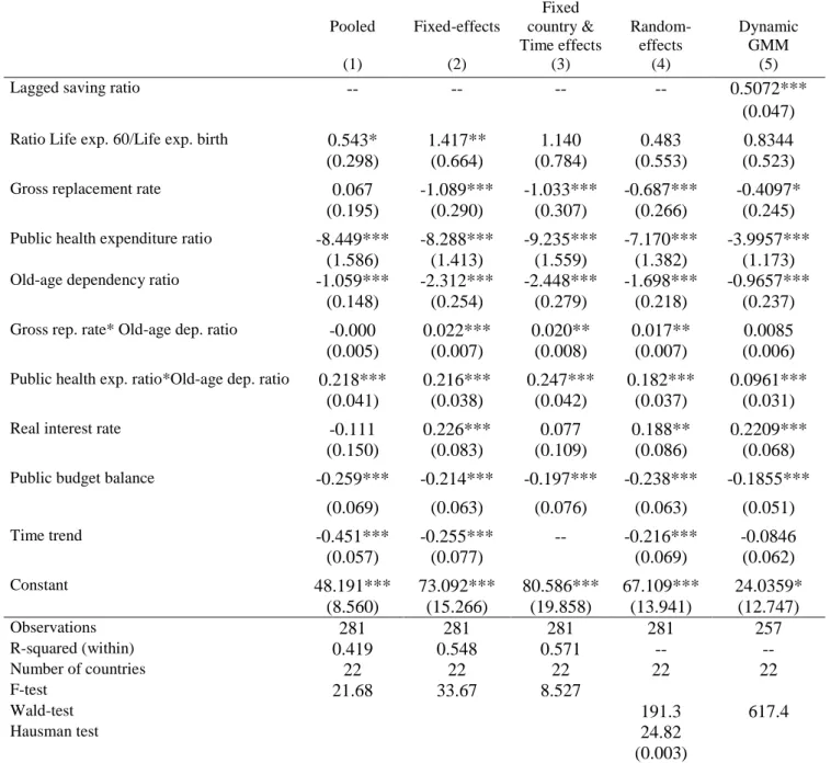
The signs of estimated coefficients appear robust, basically confirming the results from the baseline specification (equation 18). Most estimated coefficients are significant and have the expected sign (Table 1).

The sign of the life expectancy ratio is positive and significant for the pooled and fixed-effects model. This result is compatible with equation (16) above, suggesting that an increased longevity generates incentives to save.

[Table 1. Econometric estimates of household saving rate]

In line with the theoretical model, the individual effect of the replacement rate on savings is negative and significant. As well, the subsidisation of health goods impacts negatively saving rates. Also in line with the life-cycle model, an increase in the share of old-age population (60-99 years) has a negative impact on the saving rate.

The size effect of public health expenditures is large. An increase of one percentage point of public health spending to GDP induces on average almost a one-to-one decrease (0.95 percentage points) in the household saving rate.16 The effect of the replacement rate is relatively smaller. These results point towards the importance of considering both the pension and health systems among the determinants of savings. As health care provision could have a significant impact on household savings, it should be taken into account when designing health care reforms.

The interaction terms between both the replacement rates, public health expenditure and the share of old-age population are positive and significant. This suggests that the combination of high replacement rates, large shares of public health spending and old-age population could generate excess savings after retirement. For example, when old-age dependency ratios are above 45-50% the total impact of dependency ratios becomes positive. If old-age consumers shift their consumption structure towards goods that are heavily subsidised and receive substantial retirement income, both a decline in consumption expenditures and a surplus of saving at older ages could indeed be observed. Finally, the interest rate is positive and significant in the fixed-effect models. The level of the public budget balance has a negative impact on savings in all models, i.e. budget deficits tend to increase the saving rates. This result is compatible with the Ricardian equivalence, although the size of the estimated coefficient is below one indicating that there is no full compensation between public and private savings.17

5. Concluding remarks

The main novelty of this paper is to integrate health system among the determinants of aggregate savings, together with pension replacement rates and longevity. Given that the consumption bundle of old-age individuals tends to be twisted towards health goods, the systems that provide a large

16. These marginal effects were calculated using the baseline model (column 3, Table 1) and the average values for the replacement rate, public health expenditure ratio and share of old-age population given in Annex Table 1.

17. This is line with other results in the empirical literature (e.g. Serres and Pelgrin, 2003; de Mello, Kongsrud and Price, 2004).

subsidization of these goods tend to decrease household savings. This is an issue has been somewhat overlooked in the literature and policy debate.

We developed a life-cycle theoretical model combining Pay-as-You-Go (PAYG), funded pension retirement incomes and welfare transfers (e.g. public health insurance) and derived an aggregate household saving equation.

Our results are in line with the theory and highlight that the joint effect of pension and health systems should be taken into account when designing health and pension care reforms. The changing structure of consumption with age, together with a large subsidy for health goods and increasing replacement rates can explain observed patterns of household savings. Taken alone, high replacement rates and large public provision of health care contribute negatively to aggregate household savings. However, if old-age consumers shift their consumption structure towards goods that are heavily subsidised and receive substantial retirement income, this could induce both an observed decline of consumption and a surplus of saving at old ages. Confirming a Ricardian equivalence effect, we found that public budget deficits (surplus) tend to increase (decrease) household savings. Finally, in line with life-cycle theory an increase in longevity leads to increase saving.

References

Aguiar, M, Hurst E (2005) “Consumption vs. Expenditure,” Journal of Political Economy, 113(5): 919 -948.

Aguiar M, Hurst E (2009) “Deconstructing Lifecycle Expenditure”, University of Chicago,

http://faculty.chicagobooth.edu/erik.hurst/research/deconstructing_may2009.

Aisa R, Pueyo F (2013) “Population Ageing, Health care and Growth: a comment on the effect of Capital accumulation, Journal of Population Economics, 26:1285-1301.

Ando A, Modigliani F (1963) “The Life Cycle Hypothesis of Saving: Aggregate Implications and Tests”, American Economic Review, 53: 55-84.

Arellano M, Bond S (1991) “Some tests of specifications in Panel data: Monte Carlo evidence and an application to employment equations”, Review of Economic Studies 58: 277-297.

Attanasio O (1999) “Consumption”, in Handbook of Macroeconomics, Vol. 1B, Ed. by J. Taylor and M. Woodford, (Amsterdam: Elsevier Science).

Baillu J, Reisen H (1997) “Do Funded Pensions Contribute to Higher Aggregate Savings? A Cross Country Analysis”, OECD Development Centre Technical Papers 130, (Paris, Organisation for Economic and Co-operation and Development).

Banks J, Blundell R, Tanner S (1998) “Is There a Retirement-Savings Puzzle?” American Economic

Review, 88 (4): 769-788.

Barro R (1974) “Are Government Bond Net Health?”, Journal of Political Economy, 81: 1095-1117. Bernheim D, Skinner J, Weinberg J (2001) “What Accounts for the Variation in Retirement Wealth among U.S. Households?” American Economic Review, 91(4): 832-857.

Blau D (2008) “Retirement and Consumption in Life-cycle Model”, Journal of Labor Economics, 26(1): 35-71.

Bloom DB, Canning D, Graham B (2003) “Longevity and Life-Cycle Savings”, Scandinavian

Journal of Economics, 105: 319–38.

Bloom DB, Canning D, Mansfield R, Moore M (2006) “Demographics Change, Social Security Systems and Savings”, NBER Working Paper No. 12621, (Cambridge, Massachusetts, National Bureau of Economic Research).

Bohn H (1999) “Social Security and Demographic Uncertainty: The Risk Sharing Properties of Alternative Policies”, WP, University of California of Santa Barbara.

Börsch-Supan A, Reil-Held A, Rodepeter R, Schnabel R, Winter J (2000) “The German Savings Puzzle”, Universitat Mannheim Working Paper no. 01-07.

Börsch-Supan A, Lusardi A (2003) “Saving: A Cross Sectional Perspective”, in Life Cycle Savings

and Public Policy edited by Axel Börsch-Supan, 1-31, Academic Press, New York.

Bosworth B, Burtless G (2004) Pension Reform and Saving, The Brookings Institution.

Browning M, Lusardi A (1996) "Household Saving: Micro Theories and Micro Facts", Journal of

Browning M, Crossley T (2001) “The Life-Cycle Model of Consumption and Saving”, Journal of

Economic and Perspectives, 15(2): 3-22.

Bureau of Labor Statistics, Consumer Expenditure Survey, United States Department of Labor,

http://www.bls.gov/cex/csxstnd.htm.

Clark G, Strauss K (2008) "Individual pension related risk propensities: the effects of socio-demographic characteristics and a spousal pension entitlement on risk attitudes", Ageing and Society, 28: 847-874.

Callen T, Thimann C (1997) “Empirical determinants of households saving : Evidence from OECD countries ”, IMF Working Papers 97/191, (Washington, International Monetary Fund).

Caroll C (2000) Why do the rich save so much?, in Does Atlas Shrug? Ed. by Joel Slemrod, pp: 465-484, (New-York: Russel Sage Foundation and Harvard University Press).

Chakraborty S 2004, “Endogenous lifetime and economic growth”, Journal of Economic Theory, 116: 119-137.

Corsetti G, Schmidt-Hebbel K (1995) “Pension Reform and Growth”, The World Bank Policy

Reform Working Paper No. 1471, Policy Research Department, (Washington, The World Bank).

De Nardi M, French E, Jones JB (2010) “Why do the Elderly Save? The Role of Medical Expenses”,

Journal of Political Economy (118)1: 39-75.

Edward S (1996) “Why are Latin America’s Saving Rates So Low? An International Comparative Analysis”, Journal of Development Economics 51: 5-44.

Eurostat, Household Budget Survey, European Commission,

http://epp.eurostat.ec.europa.eu/statistics_explained/index.php/Glossary:Household_budget_survey_ (HBS).

Feldstein M (1974) “Social Security, induced retirement and aggregate capital accumulation”,

Journal of Political Economy 82(5): 905-26.

Fernandez-Villaverde J, Krueger D (2007) “Consumption Over the Life Cycle: Facts from Consumer Expenditure Survey Data”, The Review of Economics and Statistics,MIT Press, 89(3): 552-565. Friedman M (1957) The Theory of the Consumption Function, Princeton University Press, Princeton (New Jersey).

Hurd M, Rohwedder S (2003) “The Retirement-Consumption Puzzle: Anticipated and Actual Declines in Spending at Retirement”, NBER Working Paper No. 9586, (Cambridge, Massachusetts, National Bureau of Economic Research).

Jørgensen OH, Jensen S (2008) “Labour supply and Retirement Policy in an Overlapping Generations Model with Stochastic Fertility”, CEBR Discussion Paper 1/2009.

Scholz JK, Seshadri A, Khitatrakun S (2004) “Are Americans Saving "Optimally" for Retirement?”,

NBER Working Paper No. 10260, (Cambridge, Massachusetts, National Bureau of Economic

Research).

Loayza N, Schmidt-Hebbel K, Servén L (2000) “What Drives Private Saving across the World?”,

de Mello L, Kongsrud PM, Price R (2004) “Saving Behaviour and the Effectiveness of Fiscal Policy”, OECD Economic Department Working Papers no. 397, (Paris, Organisation for Economic and Co-operation and Development).

Modigliani F, Brumberg R (1954) “Utility analysis and the consumption function: an interpretation of cross-section data”, in Post-Keynesian economics, edited by Keneth Kurikara, Rutgers University Press.

Murphy PL, Musalem AR (2004) “Pension Funds and National Saving”, The World Bank Working

paper Series no. 3410, Washington, DC.

OECD (2011) Pensions at a Glance: Retirement income systems in OECD and G20 countries, Paris, OECD Publishing.

Oliveira Martins J, de la Maisonneuve C (2006) "The Drivers of Public Expenditure on Health and Long-Term Care: an Integrated Approach", OECD Economic Studies no. 43/2, (Paris, Organisation for Economic and Co-operation and Development).

Serres A, Pelgrin F (2003) “The decline of Private Saving rates in the 1990s in OECD countries: How much can be explained by non-Wealth Determinants”, OECD Economic Studies no. 36/1, (Paris, Organisation for Economic and Co-operation and Development).

Yaari ME (1965) “Uncertain Lifetime, Life Insurance and the Theory of the Consumer”,

Figure 1. Ratio of Public Health Expenditures to Household income 0 5 10 15 in % 1970 1980 1990 2000 France UK Sweden USA

Figure 2. Average Replacement rates (in %) in selected OECD countries

FRANCE ITALY

SWEDEN PORTUGAL

USA

Source: OECD ADB data base and authors’ calculations.

50 60 70 80 90 1980 1985 1990 1995 2000 Years 65 70 75 80 1980 1985 1990 1995 2000 Years 45 50 55 60 1980 1985 1990 1995 2000 Years 20 40 60 80 1980 1985 1990 1995 2000 Years 40 45 50 55 1980 1985 1990 1995 2000 Years

Figure 3. Public budget balances and Household Saving rates1 -2 0 -1 0 0 10 20 30 H o u se h o ld sa vi n g ra ti o (i n % ) -20 -10 0 10 20

Government net lending, as a % of GDP

(1) The sample corresponds to 22 OECD countries for the period 1970-2009 (depending on the availability of data).

TABLE 1. Econometric estimates of household saving rate1 (1970-2009, 22 OECD countries) Pooled Fixed-effects Fixed country & Time effects Random-effects Dynamic GMM (1) (2) (3) (4) (5)

Lagged saving ratio -- -- -- -- 0.5072***

(0.047) Ratio Life exp. 60/Life exp. birth _{0.543* 1.417** 1.140 0.483 0.8344} (0.298) (0.664) (0.784) (0.553) (0.523) Gross replacement rate _{0.067 -1.089*** -1.033*** -0.687*** -0.4097*}

(0.195) (0.290) (0.307) (0.266) (0.245) Public health expenditure ratio -8.449*** -8.288*** -9.235*** -7.170*** -3.9957***

(1.586) (1.413) (1.559) (1.382) (1.173) Old-age dependency ratio -1.059*** -2.312*** -2.448*** -1.698*** -0.9657***

(0.148) (0.254) (0.279) (0.218) (0.237) Gross rep. rate* Old-age dep. ratio -0.000 0.022*** 0.020** 0.017** 0.0085 (0.005) (0.007) (0.008) (0.007) (0.006) Public health exp. ratio*Old-age dep. ratio _{0.218*** 0.216*** 0.247*** 0.182*** 0.0961***}

(0.041) (0.038) (0.042) (0.037) (0.031) Real interest rate _{-0.111 0.226*** 0.077 0.188** 0.2209***}

(0.150) (0.083) (0.109) (0.086) (0.068) Public budget balance -0.259*** -0.214*** -0.197*** -0.238*** -0.1855***

(0.069) (0.063) (0.076) (0.063) (0.051) Time trend -0.451*** -0.255*** -- -0.216*** -0.0846 (0.057) (0.077) (0.069) (0.062) Constant _{48.191*** 73.092*** 80.586*** 67.109*** 24.0359*} (8.560) (15.266) (19.858) (13.941) (12.747) Observations 281 281 281 281 257 R-squared (within) 0.419 0.548 0.571 -- -- Number of countries 22 22 22 22 22 F-test 21.68 33.67 8.527 Wald-test 191.3 617.4 Hausman test 24.82 (0.003)

(1) Defined as household saving on household income. T-statistics are in parentheses, *** p<0.01, ** p<0.05, * p<0.1. The Hausman specification test of the fixed-effects vs. the random-effect model is also provided (p-value in parenthesis indicate the fixed-effect cannot be rejected at 95% confidence level).

Annex 1: Descriptive statistics of the variables used in the econometric estimates

Variable Obs. Mean Std. Dev. Min Max

Household saving ratio (in %) 786 8.49943 6.703918 -14.43505 25.96567 Ratio Life exp. 60/Life exp. birth (in%) _{1102 26.64942 1.60586 23.08239 30.65296} Replacement rate (in %) _{732 34.09579 13.10867 7.199813 66.61063} Public health exp. Ratio (in %) 417 5.287707 1.14458 1.407 7.693 Old-age Dependency ratio (in %) 1230 37.4612 8.321111 14.94235 67.14485 Real interest rate (in %) 832 2.64827 3.411264 -17.81947 16.42114 Public budget balance (in %) 862 -2.415077 4.445975 -16.00805 19.25787