Petrol Prices and Government Bond Risk Premium

Electronic copy available at: http://ssrn.com/abstract=1358901

Petrol prices and government bond risk

premiums

By

Hervé Alexandre

Antonin de Benoist

*Université Paris-Dauphine, DRM, F-75016 Paris, France ºcontact : herve.alexandre@u-dauphine.fr

Electronic copy available at: http://ssrn.com/abstract=1358901

Introduction

The emerging economies such as Brazil or China have been developing steadily since the beginning of the nineties. During this period, the issuing of government bonds by these countries has considerably increased, underlining their need for substantial investment in infrastructure and long-term projects. But, at the same time, they have had to face a series of financial crises which has greatly reduced their credit capacity and increased the spread, therefore the cost, of financing. We still don’t fully understand the determining factors of this spread and macroeconomic indicators alone cannot explain the investors’ perception of risk.

Among the factors determining the risk associated with bonds, the price of oil is one of the key elements for consideration. As S. Edwards (1985) points out, nine of the ten last recessions have been preceded by oil crises. Moreover, the volatility of the price of the barrel has strongly increased since January 1998. Indeed, the effect of variations in the price of the barrel on economic performance has been the subject of empirical studies, (Bohi, 1991; Rotenberg and Woodford, 1996; Blanchard and Gali 2007) which have shown the impact that variations in the price of the barrel can have on growth, productivity and inflation.

This article aims to analyse the impact of the price of the barrel on bond risk premiums issued by emerging economies. It is situated in the wider framework of studies on the measurement of risk associated with foreign bonds (Edwards, 1985; Min, 1998; Pan and Singleton, 2007; Blanchard, 2007). In spite of the multiplicity of works, it would seem that no empirical study has yet focussed on the effects of the price of oil on government bond risk premiums. It is this question that is dealt with here. In order to do this, a measurement model for credit spread1 _{has been developed from data} from the EMBIG index (Emerging Market Bond Index Global) of seventeen countries. An analysis in time series has been carried out on each country, then a panel analysis, in order to determine the global impact of oil on the risk perceptions of investors. Finally, our analysis has put in place a new estimator for the price of oil which takes into account the effect of the variance of this price thus responding to recent empirical studies which have shown that the reduction of the impact of the price of petrol is partly the result of an increase in the volatility of the price of the barrel (Blanchard and Gali, 2007)2_.

1_{This spread corresponds to the difference between the yield of a risky bond and that of one which is virtually}

risk-free such as the treasury bills issued by the US.

1.

Literature review

1.1. Factors determining the risk associated with government bonds

During the nineties, the issuing of government bonds in emerging countries has considerably increased, improving the terms of exchange and the liquidity of this type of financial product. Today it is the primary source of finance in developing countries after direct investment abroad. At the same time the public-debt market in the developing countries has experienced serious upheavals following several financial crises. In these conditions, it is important to understand the factors determining the prices of government bonds.

1.1.1. Theoretical models for spread measurement.

Government bond yield is an indicator of the economic fragility of a country. It is a pertinent measure of a country’s risk of defaulting as perceived by the investors and of its capacity to turn to external sources of finance. However, the level of the spread (if it is a function of the principal risks such as compensation, liquidity and market), is determined by a multitude of other factors that are difficult to identify. There are two distinct forms of models: structural models and reduced-form models.

Certain studies maintain a structural approach to spread measurement based on the model of Hull and White (1990). According to certain works such as those of Duffie and Singleton (1999), Dai and Singleton (2003), Pan and Singleton (2007), the arbitration of credit default premium Swap (CDS) on government bonds can be expressed in terms of probability of negative default risk and the sums of losses in case of default. The probability of default is endogenous and depends on the average maturity of debts and the no-risk interest rate. The resources are made up of international reserves and the value of the state’s budget.

The reduced model forms deduce the value of the bond by updating the future contractual flows of the bond. Contrary to preceding models, the probability of default and the collection ratio are exogenous. They are estimated based on credit ratings and macro-economic indicators that influence the solvency of the borrower. Models for measuring the spread use the logarithm for government bonds spread rather than their level (Edwards, 1985). The relationship between the risk premium and the default probability can be written in the following way:

s=

[

where s represents the spread, p represents the default probability and γ, a parameter. The author assumes that the default probability takes the following form:

p= exp

∑

∑

where αi and yi are the determinants of the default probability. We can thus obtain the form of the spread:

log s_ti=α_ti

∑

k=1 K

β_tikX_tik+ε_tik

Where sti is the level of spread of the country I, on the date t, a variable I, among k, independent variables, and εit, _{the residual error.}

The empirical study which will constitute the second part of this study is based on this form of model.

1.1.2. Macro-economic determinants

Different models allow for the selection of macro-economic k variables from a modelling of the borrowing status of a country. The principal indicators of solvency are weak stock of debt, weak interest rate or production growth. The level of openness of the economy is another key factor in the international solvency of the country. Other variables of competitiveness such as the exchange rate can play an important role in the credit risk of countries.

One of the founding articles of empirical literature on the international credit markets is that of Edwards (1985). He is particularly interested in the measurement of government bonds in the context of the debt crises of the eighties. He develops a model that considers the emerging countries as small borrowers within an almost perfect financial market: the spread depends on the default probability which itself results from macro-economic variables.

The data comes from the World Bank and the International Monetary Fund (IMF) and concerns 727 debt instruments of 19 of the least developed countries covering the period from 1976 to 1980. Several determining factors are considered: the ratio of investment growth as a percentage of GDP,

the average amount to be invested, the growth of GDP per unit of capital, the rate of inflation, international reserves, the deflation rate, and government spending added to GDP.

The empirical results show that the development of the spread takes into account the economic characteristics proper to the countries under consideration. For example the debt-to-GDP ratio is positively correlative to the spread level. Also, the sum of international reserves is significant and plays an important role in determining the amount of the risk premium. The proportion to invest has a negative impact on the default probability and the spread of government securities. The study shows that temporal differences within the same country are more important than the differences between countries. Edwards concludes from this that investors have taken the individual macro-economic specificities of countries into account.

Canter and Packer (1996) analyse the determinants of the government bonds spread in over 49 countries in 1995, taking account of the growth in GDP, inflation, current account, debt, indicators of economic development and agency ratings (Moody’s, Standard, and Poor’s). The authors do not find any significant relations between the macro-economic indicators of the countries and the fluctuations in the spread.

An empirical study by Kamin and van Kleist (1997) analyses more than 304 state securities issued in the nineties. They find that the spread in Latin American countries is, on average, more than 39% higher than those in Asia. This result points to a segmented government bonds market.

Min (1998) carried out an empirical study from 1991 to 1995 to analyse the economic determinants of the yield from government bonds made out in American dollars in the emerging countries. The determinants of default probability are regrouped into four groups of variables that explain the spread level: liquidity and solvency, basic macro-economics, variables of external shocks and indicative variables. The results show that the liquidity and solvency of the economy play an essential role through GDP-to-debt ratio, and the ratio of international reserves to GDP, and integrates the effect of external shocks on the risk of default by a country3_{. Most of the regional} specificities are not significant which indicates that common factors determine the spread level. This result is confirmed by recent studies such as those by Longstaff and Coll. (2007). Finally, it shows that the volatility of the spread is symmetrically influenced both by liquidity and by macro-economic fundamentals such as the rate of inflation, the GDP-to-debt ratio and the ratio of international reserves to GDP.

3 _{Barr et Pesaran (1997), among others, have shown the role of conditions of international liquidity and}

fluctuations in interest rates in the movement of capital during the nineties. Eichgreen and Mody showed the vulnerability of the spread of emerging countries to international financial conditions.

Following the increase in the volatility of sovereign debt at the end of the nineties, many investors appeared on the market to take advantage of investment opportunities. Goldman and Sachs (200) were the first to establish an arbitration model on bond spreads issued in fifteen emerging economies from 1996 to 2000. In the same way as Min (1998), Goldman and Sachs (2000) break the macro-economic variables down into four categories: solvency (real GNP), liquidity (Debt/PIB, International reserves, Budgetary balance/GNP, LIBOR), external shocks (exchange rate, exports/GNP) and indicative variables (previous default). From the evaluation model, it would seem that twelve of the fifteen countries considered had undervalued bonds while only one country reached its basic value.

Eichengreen and Moody (1998) analysed more than 1300 bonds issued by 55 emerging economies between 1991 and 1997. The explanatory factors of the spread are the ten-year interest rate on American bonds, the ratio of external debts to GDP, the ratio of debts to exports, the ratio of international reserves to GDP, the level of growth to GDP and finally budget deficit to GDP. Their result confirmed that an increase in the quality of a country’s credit increases the probability of bond issuing and reduces the government bond premium. The market differentiates between the issuing countries as a function of the quality of the borrower.

Pesaran and Coll. (1999) favour an error-correction model which makes it possible to explain the spread level by long-term factors while analysing the determinants of the short-term dynamic of the yield on bonds from emerging countries. More than half of the spread variations can be explained by macro-economic indicators.

Ferruci (2003) is interested mostly in the proportion of the development of the market spread explained by the fundamentals of macro-economics. The impact of interest rates on short-term treasury bills from the United States is positive; the impact on long-term treasury bills is negative.

1.1.3 Government bonds: a class of assets in its own right?

Is the risk associated with government bonds merely idiosyncratic or rather determined by global economic factors?

To answer this question, Longstaff and Coll. (2007) studied the profile yield/risk of government bonds. The interest of their study is to analyse the determinants of credit risk relating to government bonds in the context of analysis of the model of evaluation for financial assets (MEDAF). The empirical study concerns the monthly data of CDS premiums made out in US dollars between October 2000 and May 2007 for each of the 26 countries studied. The CDS premiums have the

advantage of directly reflecting the risk worries of investors. Moreover, the CDS government bonds market is often more liquid than that of the bonds to which they refer.

In order to analyse the determinants of the development of the CDS government bonds premium, the authors include four categories of explicative variables: the local variables, (the yield of the local market, the exchange rate and the sum of reserves), the financial variables of the market which concern the asset market and American bonds, the variables of global risk premiums, (yield of the S&500 index, variation of the spread between the historic volatility and estimated on the options of the VIX index), and an investment flow variable.

Their results reveal a very strong correlation between the CDS premiums of the different countries: Three principal global factors explain 50% of their variation. The spread of the CDS on government bonds depends on American shares S&P 500 and NASDAQ indices), on the bonds market and on a global risk premium. Pan and Singleton (2007), show that the spreads of different countries are strongly correlated with the VIX index. The global risk, identical in the 26 countries, determines more than 30% of the total development of the CDS spreads on government bonds. The macro-economic determinants specific to the country only represent a small part of the total development of premiums. The CDS premium is grouped according to geographical zones. As in the work of Min (1998), or Ferruci (2003), it would seem that the risk premiums are higher in Latin America than in the other continents. The liquidity of CDS also has an impact on the nature of risks associated with government bonds.

Government bonds are the object of four types of macro-economic risks : Insolvency, illiquidity, external shocks and basic macro-economics.

1.2. Impact of oil prices on growth, inflation and productivity

To begin with, an oil crisis results in a large reduction in the supply of oil , which gives rise to political events that are exogenous to the oil market and macro-economic conditions.

1.2.1. Oil crisis and economic performance: the facts

Economists have long been examining the relation between the price of petrol and macro-economic performance. Their interest in the subject dates from the seventies, an era that was marked by a growing dependence on oil-importing economies, the fluctuations in the price of the barrel and the relatively weak economic performance of the United States. Since then, many oil crises have occurred: the crash in 1986, the increase of 1990-1991 associated with the Gulf war, the growth of

2000 and the crisis of 2003 associated with the war in Iraq. In 2007-2008 the price of oil strongly increased resulting from a conjunction of economic, political, geological and climatic factors.

Thus the variations in the price of petrol depend to a large extent on exo genous events such as those linked to the political situation in the Middle East, the development of cartels or military conflicts. The increase in the price of petrol is deemed responsible for recessions, inflation and for t he reduction in productivity of the mid-seventies. Numerous empirical studies such as that of Hamilton (1983) have shown that the relation between the price of petrol and GDP is more than a simple statistical coincidence. Determining the mechanisms by which the price of petrol influences macro-economic performances is essential to quantify the impact of oil prices on the solvency of a country and to measure the spread of sovereign bonds. Nevertheless, this idea has been called into question by certain economists (Barsky and Kilian, 2002) who believe that macro-economic variables partly determine the fluctuations in the price of petrol.

1.2.2. Mechanisms by which the price of oil influences growth, inflation and productivity. 1.2.2.1. The effect of energy consumption on GDP

The elasticity of production in relation to energy depends on the proportion of energy in production. Empirically, this proportion is relatively small. For example, in 2000, in the United States, the consumption of oil barrels which reached 7.2 million bar rels only represented 2.2% of GDP. However, it is important to point out that this percentage has since risen substantially following recent rises in the price of petrol, yet remain small in relation to production.

Nevertheless, the relations of cause and effect between the variatio ns in the price of petrol and GDP are far from simple. Bohi (1991) shows that there is no empirical evidence which supports the idea that countries with higher energy costs are more severely affected by an oil crisis than countries who are less reliant on oil as a source of energy. The empirical data shows in fact that in terms of growth, the cost of an oil crisis is not so much the result of an increase in the price of petrol, as that of a reduction in the consumption of other factors of productions that it leads to. So an increase in the price of petrol can bring about a reduction in the wage bill which can have important effects on growth. Rotemberg and Woodford (1996) show that an increase of 10% in the price of petrol can result in a reduction of 2.5% of GDP over an eighteen month period.

1.2.2.2. Sectoral reallocations

An oil crisis can have a different impact upon capital and employment, and can cause a reallocation between sectors of activity. Hamilton (1983 ) shows that oil crises cause a reduction in demand in other industries such as the automotive industry. This variation in demand brings about a redistribution of wok between the sectors of activity. According to Bernanke (1983) an increase in the price of petrol causes companies to postpone their investment while they wait to know if the increase in the price of the barrel is temporary or permanent. Evidently, such uncertain effects only have a relatively slight impact on the magnitude of a recession.

The costs of capital adjustment and work, following an oil crisis, have been the subject of much research. Lee and Coll. (1995) find that GDP predictions in the OECD countries are much better when dividing the price of petrol by its volatility.

1.2.2.3. Monetary policies and inflation

Certain studies highlight the role of monetary policy in the relation between the price of petrol and GDP. According to Barsky and Kilian (2002, 2004), the recession of 1973-1974 was one of the consequences of the monetary expansion of the US federal reserve in order to respond to fears about inflation which resulted in an increase in the price of the barrel. Monetary policies can also cause inflationary spirals, wages-prices, caused by the price of petrol (Bruno and Sachs, 1985).

The macro-economic effect of an increase in the price of the barrel can potentially result in stagflation. This phenomenon is particularly important as an explanation of the crisis of the seventies. As the rate of inflation is linked to monetary policy, the impact of an oil crisis depends primarily on the reaction of central banks to this economic shock. Hooker (2002) illustrates this phenomenon by showing that oil crises significantly contributed to causing inflation in the US up to 1981, the date on which the question of inflation became a priority of monetary policy.

1.2.2.4 Development of mechanisms over time

While the economies of OECD countries have seen real variations in the price of oil in 2000 and 2003 which were as serious as the oil crises of 1973 and 1979, no variation in GDP and the rate of inflation were recorded. This fact calls into question the mechanisms put in place with regard to the relation between the price of oil and macro-economic performances.

Blanchard and Gali (2007) confirm the hypothesis that the price of petrol influenced the stagflation of the seventies, but point out that other effects were at work. The also establish that the mechanisms for transmission have developed since the seventies. Globally , the economies and notably those of the OECD are a lot less sensitive to fluctuations in the price of the barrel. The impact of a variation in the price of oil on the inflation rate has weakened. Several explanations can be given for this. On the one hand, inflexible wages has diminished. They generated a balance between the stabilization of inflation and production. A greater flexibility in the job market and salaries partly explains the reduction of the impact of fluctuations in oil prices. On the other hand, the central banks have actively adopted a policy of maintaining a low rate of inflation since the beginning of the eighties, giving credence to the objectives of monetary policy (Herrera and Pesavento, 2007). Finally, the share of energy consumption and the dependence of economies on oil has dropped, even though there are disparities according to the country concerned.

1.2.3. Price of oil and economic risk: the case of oil producing countries

Most studies have focussed on oil importing countries. However, the relation between economic performance and the price of the barrel is radically different in an oil-producing country. Mechanically, an increase in the price of oil should increase revenue in the economy and result in an increase in GDP. This connection is questioned by the efficiency of wealth redistrib ution systems, controversial empirical result findings and economic development models.

The model of Corden and Neary (1982), known as “Dutch disease”, predicted that an important increase in oil revenues can damage the GDP of certain developing countries. This model was empirically backed up in oil-producing countries during the seventies. The production of oil was developed to the detriment of the manufacturing and agricultural sectors.

It is certain that the price of the barrel influences the credit risk of all governments. If the relation between the price of oil and macro-economic performance has developed since 1980, (Blanchard 2007), it remains significant. However no empirical study has specifically sought to study the impact of the price of oil on the Government bonds spread. This is specifically the subject of the second part of our article.

2.

Empirical study

The objective of the empirical study is to quantify the impact of the development of oil prices on the risk premium of government bonds. To do this, after the presentation of some descriptive statistics, we will proceed with an analysis in time series on each country considered, then to a panel analysis.

2.1. Analysis of the database

A preliminary analysis of the database makes it possible not only to set the framework for the empirical study, but also to choose adequate tools to proceed with the estimate. The data from the empirical study consists of government bond spreads across fourteen emerging countries and four regions, Latin America, The Middle East, Asia and Africa. The data is daily and is obtained from DataStream databases with the exception of the WTI rate which is supplied by Reuters. The period covered is almost ten years from the 1st January 1998 to the 30th May 2008.

The government bond spread refers to the risk premium that the bond holder demands from the seller to hold the bond. For bonds issued at par, the spread corresponds to the difference between the interest rate of the bond and the no-risk interest rate , as is the case with the interest rate of bonds from the American treasury.

We will use the EMBIG index published by JP Morgan which is an index of the spread of government bonds from emerging countries made out in US dollars. This index measures the difference between the premium paid by the emerging countries and that of an American treasury bond of similar maturity. It is calculated from the average of all the bonds weighted by the capitalisation of the bonds market, in contrast to the EMBI index (Emerging Market Bond Index) which includes only liquid bonds including Eurobonds and Brady bonds whose minimum face value is 500 million US dollars. The EMBIG index is of a maturity higher than two and a half years and covers more than 27 countries since 1998 (the EMBI index covers five countries from 1991 to 1995 and 11, since 1995).

Including the two series in the same empirical study creates a selection bias because the EMBI index only covers Brady-type bond yields and the yields on certain structured instruments. Moreover, these two indices EMBI and EMBIG can also give different risk measurements because of the fact that the composition of the two bond portfolios is different. The empirical study

developed in the present study only includes EMBIG indices: their quantity is largely sufficient to bring the empirical estimation to a satisfactory conclusion.

Graph 1 presents the fluctuations in the EMBIG index for the four main regions analysed: the Middle East, Africa, South America and Asia. The EMBIG index allows for a more pertinent geographical analysis by region rather than by country. The indices by region are calculated as a geometrical average of the country indices. It of noteworthy significance that in the group pf regions studied, the government bonds spread increased strongly from January 2001. In Africa, this increase was higher than in the other regions: it went from 231 points in January 2001 to 518 points in April 2008.

During the same period, the EMBIG indices of Asia and South America also increased but to a lesser degree than in Africa. Concerning the countries of the Middle East the increase of the government bonds spread is low during the entire period under consideration and the spread only reached 255 base points in April 2008.

Graph 1: Development of the EMBIG index by region from 1998 to 2008

2.1.1. Explanatory variables

As far as explanatory variables go, our study draws on the models studied in the first part. The EMBIG index makes it possible to obtain data gathered over several decades which is not the case in most macro-economic series.

Africa

Latin America Asia

In their study, Longstaff and Coll (2007) show that the yield in excess of the risk corresponds to a remuneration of the global risk determined by external factors. This is why our analysis has focussed on those variables stemming from external shocks. Three groups of independent variables have been included in the model: the market risk variables, exchange rates and external shocks. The market risk is interpreted by two indices: the Chicago Board Options Exchange Volatility Index (VIX) and the S&P500 index. The VIX index is a measure of the implicit volatility of a bond in the S&P500 index. It concerns the perception of risk by the investors. The volatility history of the market is not considered. An increase in the VIX index is explained by an increase in the bonds spread. Pan and Singleton (2007) show that the premium bonds of the different countries are strongly correlated to the VIX index and, more generally, to the S&P500 index, a factor of global risk. Our empirical study supposes that these two indices have positive impacts on the spread.

The interest rate of the country by dollar unit (USD), noted as FX, is included in the model. It reflects both the competitiveness of the economy and the solvency of the country. These two factors have a distinct impact on the spread. An increase in the exchange rate reduces the competitiveness of a country and increases the EMBIG index, while an increase in the exchange rate increases the ability of a country to fulfil its contract and thus reduce the bond risk premium.

The external shocks are highlighted in this study by two indicators, international l iquidity and the price of oil. An increase in the interest rate increases the cost of new finance and debts that have already been contracted. Eichgreen and Mody (1998) confirmed this result. The impact of international liquidity is analysed by the interest rate over a three month period or short-term interest rate (STI), and the ten-year interest rate or Long Term Interest Rate (LTI) of the US treasury bonds. In conformity with the results of Ferruci (2003), the impact of the STI should be positive while that of the LTI should be negative.

If international liquidity has been a subject of interest that has been well discussed in financial literature, the impact of the price of oil has not excited anything like the same interest. The article by Min (1998) is, to our knowledge, the only article which includes the price of petrol as an explanatory variable in the model he uses. However the author does not find significant links between the variations in the price of oil and government bond spreads.

2.1.2 Impact of the price of oil

The impact of the price of oil economic performance has been the object of a detailed literary review. It suggests that the price of the barrel has a negative impact on the economies of oil-importing countries. Contrastingly, the result is less obvious for oil-producing countries.

The variation in the price of oil is represented by the West Texas Intermediate (WTI), also known as the Texas Light Sweet. The WTI index is an index of light crude oil which serves as a yardstick for establishing the average price of oil from America. Economic theory suggests studying the real price of oil rather than its nominal price. Nevertheless, while taking account of the high range of fluctuations in the price of oil and the low inflation rate over the period considered, the fact of using the real price or the nominal price of oil does not interfere with the estimation of the spread. In the tradition of most empirical studies, our estimation adopts a nominal price level in logarithm form, noted as LN (WTI).

2.1.3. Descriptive statistics

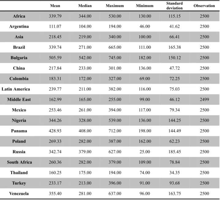
Tables 1 and 2 present the statistical description of all the variables that are of interest.

The average differs greatly according to the country and the region. Therefore with an average EMBIG index of more than 509.59, the bonds issued by Bulgaria show the highest spread in the sample. Contrary to this, with an EMBIG index average at 111.07, Argentina has the lowest spread of the countries and regions covered in this study.

The variance is also very mixed according to the country. Argentina shows the weakest standard deviation, that is, 41.62, while Russia shows the strongest at 185.45. It would seem that the countries that have the highest average level of Government bond spread have a particularly high variance.

Table 1: Statistical description of dependent variables

Mean Median Maximum Minimum Standard _deviation Observation

Africa 339.79 344.00 530.00 130.00 115.15 2500 Argentina 111.07 104.00 194.00 46.00 41.62 2500 Asia 218.45 219.00 340.00 100.00 66.41 2500 Brazil 339.74 271.00 665.00 111.00 165.38 2500 Bulgaria 505.59 542.00 745.00 182.00 150.12 2500 China 217.84 233.00 301.00 136.00 47.72 2500 Colombia 183.31 172.00 327.00 69.00 72.25 2500 Latin America 239.77 211.00 382.00 116.00 75.03 2500 Middle East 162.99 165.00 255.00 99.00 46.12 2499 Mexico 253.46 261.00 394.00 117.00 79.34 2500 Nigeria 344.26 328.00 539.00 136.00 144.25 2500 Panama 428.93 408.00 712.00 198.00 144.49 2500 Poland 269.33 282.00 387.00 162.00 62.23 2500 Russia 342.74 379.00 627.00 25.00 185.45 2500 South Africa 260.36 282.00 379.00 109.00 78.84 2500 Thailand 160.25 175.00 194.00 74.00 34.35 2500 Turkey 233.17 213.00 396.00 91.00 93.68 2500 Venezuela 355.40 281.00 637.00 96.00 163.75 2500

Table 2: Statistical description of independent variables

Variables Mean Median Maximum Minimum Standard deviation Observations

WTI4 _{41.16 31.85 121.57 10.73 22.46 2 610} VIX Index 20.29 20.00 45.00 9.00 6.86 2 717 S&P 500 1, 217.88 1, 215.81 1, 565.15 776.76 176.77 2 618 Short-term interest rate5 3.53 3.94 6.42 0.61 1.71 2 584 Long-term interest rate6 6.62 6.46 9.09 4.16 1.02 2 717

The short-term risk-free interest rate (STI, 3 months maturity) is lower than the long term risk free interest rate (LTI, maturity 30 years). This leads to the conclusion that the structure by term of interest rates is a growth function of the maturity.

A unit root test (Augmented Dickey-Fuller test) was carried out on each time series sample. It transpires that the government bonds spread is part of a first order integration (1).

2.2. Estimation and Interpretation

2.2.1. Analysis in time series for each country

In the first instance the study proceeds by a time series analysis of government bond spread for each country and region. This makes it possible to rely on the impact of the price of oil on the EMBIG index on the idiosyncratic situation of the country under consideration. The model is an estimate by the least squares of the form;

Where:

LTI is the Long Term Interest Rates STI is the Short Term Interest Rates WTI is the West Texas Index

4_{WTI signifies West Texas Instrument Intermediate}

5_{American treasury bills with three-month interest rate.}

6_{American treasury bills with thirty year interest rate.}

Log(EMBIGit) - Log(EMBIGit-1) = βi1(STIt – STIt-1) + βi2(LTIt – LTIt-1) + βi3(VIXt – VIXt-1) + βi4(S&P500t – S&P500t-1) + βi5(Log(WTI)t – Log(WTI)t-1) + εit (1)

VIX is the Chicago Board Options Exchange Volatility Index

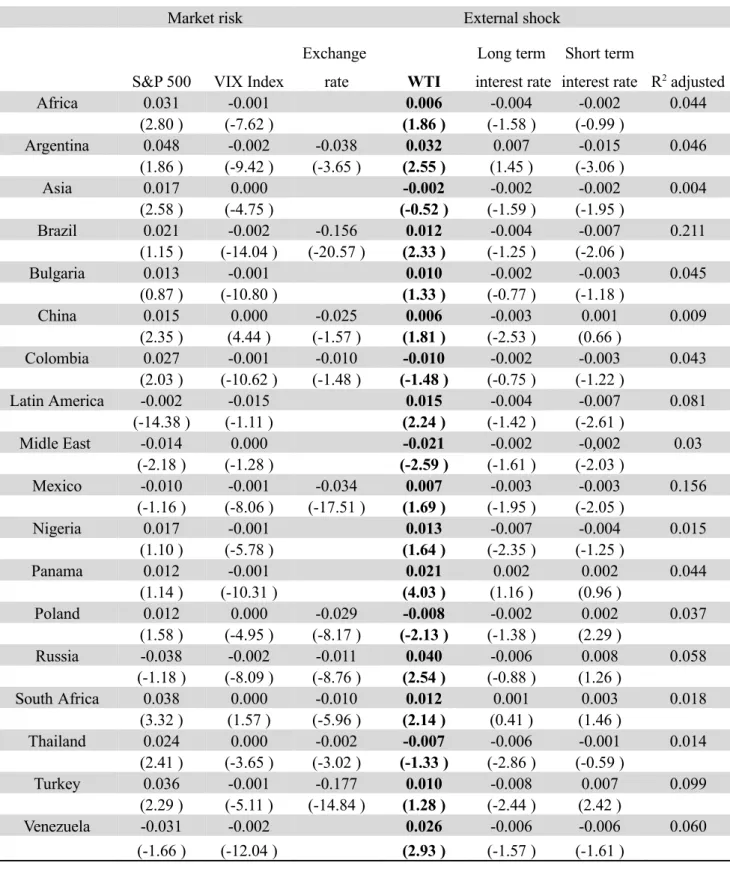
Table 3 shows the results of this model, that is to say, the impact of independent variables on the EMBIG index logarithm.

Table 3: Impact of independent variables on the EMBIG index

The adjusted t-stats of the White correction are presented in brackets below the coefficient.

Market risk External shock

S&P 500 VIX Index

Exchange

rate WTI

Long term interest rate

Short term

interest rate R2 _adjusted

Africa 0.031 -0.001 0.006 -0.004 -0.002 0.044 (2.80 ) (-7.62 ) (1.86 ) (-1.58 ) (-0.99 ) Argentina 0.048 -0.002 -0.038 0.032 0.007 -0.015 0.046 (1.86 ) (-9.42 ) (-3.65 ) (2.55 ) (1.45 ) (-3.06 ) Asia 0.017 0.000 -0.002 -0.002 -0.002 0.004 (2.58 ) (-4.75 ) (-0.52 ) (-1.59 ) (-1.95 ) Brazil 0.021 -0.002 -0.156 0.012 -0.004 -0.007 0.211 (1.15 ) (-14.04 ) (-20.57 ) (2.33 ) (-1.25 ) (-2.06 ) Bulgaria 0.013 -0.001 0.010 -0.002 -0.003 0.045 (0.87 ) (-10.80 ) (1.33 ) (-0.77 ) (-1.18 ) China 0.015 0.000 -0.025 0.006 -0.003 0.001 0.009 (2.35 ) (4.44 ) (-1.57 ) (1.81 ) (-2.53 ) (0.66 ) Colombia 0.027 -0.001 -0.010 -0.010 -0.002 -0.003 0.043 (2.03 ) (-10.62 ) (-1.48 ) (-1.48 ) (-0.75 ) (-1.22 ) Latin America -0.002 -0.015 0.015 -0.004 -0.007 0.081 (-14.38 ) (-1.11 ) (2.24 ) (-1.42 ) (-2.61 ) Midle East -0.014 0.000 -0.021 -0.002 -0,002 0.03 (-2.18 ) (-1.28 ) (-2.59 ) (-1.61 ) (-2.03 ) Mexico -0.010 -0.001 -0.034 0.007 -0.003 -0.003 0.156 (-1.16 ) (-8.06 ) (-17.51 ) (1.69 ) (-1.95 ) (-2.05 ) Nigeria 0.017 -0.001 0.013 -0.007 -0.004 0.015 (1.10 ) (-5.78 ) (1.64 ) (-2.35 ) (-1.25 ) Panama 0.012 -0.001 0.021 0.002 0.002 0.044 (1.14 ) (-10.31 ) (4.03 ) (1.16 ) (0.96 ) Poland 0.012 0.000 -0.029 -0.008 -0.002 0.002 0.037 (1.58 ) (-4.95 ) (-8.17 ) (-2.13 ) (-1.38 ) (2.29 ) Russia -0.038 -0.002 -0.011 0.040 -0.006 0.008 0.058 (-1.18 ) (-8.09 ) (-8.76 ) (2.54 ) (-0.88 ) (1.26 ) South Africa 0.038 0.000 -0.010 0.012 0.001 0.003 0.018 (3.32 ) (1.57 ) (-5.96 ) (2.14 ) (0.41 ) (1.46 ) Thailand 0.024 0.000 -0.002 -0.007 -0.006 -0.001 0.014 (2.41 ) (-3.65 ) (-3.02 ) (-1.33 ) (-2.86 ) (-0.59 ) Turkey 0.036 -0.001 -0.177 0.010 -0.008 0.007 0.099 (2.29 ) (-5.11 ) (-14.84 ) (1.28 ) (-2.44 ) (2.42 ) Venezuela -0.031 -0.002 0.026 -0.006 -0.006 0.060 (-1.66 ) (-12.04 ) (2.93 ) (-1.57 ) (-1.61 )

The White test (1980), carried out on each regression , has a very weak p-value: it rejects the null hypothesis of absence of heteroscedasticity. The t-stats presented are therefore adjusted by the correction of White which makes it possible to have a consistent covariance matrix estimator and a direct test for heteroscedasticity. The F-tests carried out on each equation show that the groups of coefficients are significant at the threshold of 5%. The R2 _{values are relatively weak which is partly} due to the fact that the regressions are carried out in first difference.

First of all, the price of oil is a significant indicator of the global risk of external factors (Table 3). The majority of coefficients are positive and significant at the threshold of 5%. Any increase in global risk has a knock-on effect on the bonds market. For example, the spread of a country like Mexico increases in the case of an increase in the price of the barrel . An increase in the price of oil increases the perception of global risk by investors whatever the individual characteristics of the country and the EMBIG index level.

In addition the effect of the price of oil differs greatly according to the country. Russia, Argentina and Venezuela are the three countries for which the impact of the price of the barrel on spread is the highest. An increase of 1% in the price of oil manifests itself by an increase in the EMBIG index of 0.04% in Russia and 0.03% in Venezuela. The price of oil has a negative impact on the EMBIG index for the regions of Asia, the Middle East and countries such as China.

The results show that the development of the price of oil has a different impact depending on the country studied. This difference could be explained by the fact that that certain countries import oil while others export it. An increase in the price of the barrel constitutes a financial burden for the former and a benefit for the latter. This transfer of wealth could have an impact on the default probability and the losses associated with it for the borrowing countries.

With regard to the other explanatory variables (VIX, S&P500, STI, LT I), our estimate partly confirms the empirical results reviewed in the first part of our study, with the exception of the VIX index. This index of market risk has a coefficient which is negative most of the time and significantly on the threshold of 5%. This result could be explained by the migration of investors towards government bonds which are relatively low risk following an increase in risk in the stock market. The influence of the S&P500 index is positive and significant. The effect of the exchange rate on the EMBIG index is negative and significant. This seems to indicate that an increase in the exchange rate is synonymous with an increase in solvency rather than a drop in competitiveness. Finally, the sign of the long-term interest rate concurs with the results of Ferruci (2004).

2.2.2. Panel Analysis

The previous study gives an insight into the individual impact of the price of the barrel on the EMBIG indices of each country. It would be interesting to design a model that can quantify this impact from a global point of view. The question would therefore be to know what effect an increase in the price of the barrel could have on the government bonds spread.

The databases that we have used for this study have the advantage of following more than 17 countries and regions, on a daily basis, during almost ten years from January 1998 to April 2008. At the outset, the study put in place a panel analysis which it was necessary to improve on in a second part. Model (2a) used is of the form:

log









The number of observations is 25.669 and the number of groups, 17. Table 4 shows the results of the panel analysis. The procedure consists at first with the assumption that the best model is one with random effect and then secondly to consider a model with fixed effect. The t-stats are indicated between brackets below the coefficients.

Table 4: Results of the panel analysis 2a

Explained variables : (EMBIG) log

Explanatory variables1_{Random effect modelFixed effect model}

Constant 4.90169 4.90171 (-58.47) (150.63) STI -0.02093 -0.02093 (-11.32) (-11.32) LTI -0.04473 -0.04473 (-7.36) (-7.36) S&P500 0.00016 0.00016 (8.48) (8.48) VIX 0.00265 0.00265 (6.45) (6.45) Log(WTI) 0.29838 0.29838 (96.68) (96.69) Σ 0.31851 0.32599 Error 0.29196 0.29196 R2 _{within 0.63960 0.63960} Number of Observations 25669 25669

Note 1: STI signifies Short Term Interest Rate; LTI, Long Term Interest Rate; S&P500, Standards and Poor 500; VIX, Chicago Board Exchange Volatility Index; σ, random effect fixed effect.

In the case of a fixed effects model, the most relevant R² value is the R2 _{within because it gives an} idea of the intra-individual share of the dependent variable explained by the explanatory variables. The R2 _{within is 0.6396 which is very satisfactory. The R}2 _{between (0.1044) gives an idea of the} contribution of fixed effects to the model.

In order to determine which of the two models is the most relevant, we can go back to using the Haussmann test whose hypotheses are as follows:

H0: the random models are equivalent.

Ha: the fixed-effect model is better than the random effect model.

The application of this test makes it possible to reject the nul l hypothesis according to which the models are equivalent. Here the most relevant model is the fixed-effect model.

If the test makes it possible to categorize between the two models, th e model carried over must depend on other more theoretical considerations. Allowing for the existence of random effects comes back to the supposition that the factor representing the individual effects is not correlated with the explanatory variables. This hypothesis is particularly strong for our model and, consequently, the fixed-effect model is the more appropriate one for our study.

2.2.2.1 Interpretations

The panel analysis makes it possible to show that the price of the barrel has a significant effect on the EMBIG index. An increase of 1% in the price of oil brings about an increase in the spread of 0.298%.The coefficient of the price of the barrel is significantly on the threshold of 1%. The development of the price of oil is a factor of global and external risk which influences the cost of credit of all the governments.

With regard to the other explanatory variables, the empirical study rejoins the results suggested by theory and empirical literature. As Ferruci (2004) shows, the long-term interest rates have a weaker impact than the short-term rate. The VIX index has a positive and significant effect on the EMBIG index. The influence of the S&P500 ind ex on the explanatory variable is relatively weak. This can be explained by the fact that the market risk is already represented by the volatility of the options of

the S&P500 index, graded VIX. Finally σ corresponds respectively to the fixed effect and the random effect of the models.

Numerous empirical studies, such as that of Blanchard and Gali (2007), have shown that the effect of oil prices on macro-economic performance has significantly dropped since the eighties. Certain studies explain this development by an increase in the variance of the price of oil. In the following panel analysis that we have carried out, the empirical study makes it possible to construct an index of the price of oil that is corrected of volatility.

2.2.2.2 Estimator of the volatility of the price of oil.

The literature review has shown that the impact of an oil price increase on economic activity has dropped since the eighties. In fact, it is the mechanisms of transmission of oil crises on economic performance that have fluctuated. The literature shows the important role of the volatility of the price of oil on the economic performance of a country7_.

A study developed by Lee and Coll (1996) shows that the relation between economic performance and the price of oil is no longer significant since 1986. The authors defend the idea that the price of oil has not lost its influence on GDP if we take into account the extent of variations in the price of the barrel. The crises relating to oil prices are more likely to have an influence on economic performance in an environment of stable oil prices than in an environment where the movements of the price of the barrel are erratic.

Lee et al. (1996) developed an indicator of the price of petrol corrected of its variance. The authors note that this indicator significantly influences macr o-economic performances regardless of the period under consideration. This result concurs with the idea that the impact of the price of oil on economic activity is different according to whether or not it is anticipated.

Following the example of numerous empirical studies such as that of Hamilton (1996), Lee and Coll. (1996) state that the effect of the price oil is asymmetrical: an increase in the price of the barrel is associated with a significant drop in GNP, while a drop in the price is not significantly linked to economic activity. This is why we will use a positive semi-variance.

In the present study, we have put in place an indicator which concurs with the empirical results on the nature of the impact of the price of oil on economic activity. From this point of view, the indicator appears as a risk premium of oil which takes into account the volatility of the oil price oil.

This variable, noted as WTI premium, is defined by the relation between the yield of the WTI index and a positive three-month semi variance:

PrimeWTI= WTI

T−1

∑













An increase in the price of petrol is just as likely to influence the risk premium of government bonds as its variance is weak. This leads us to conclude that such a variable has a positive and significant impact on the measurement of government bonds spread.

We then proceeded to a panel analysis whose results are shown in Table 5. The method of estimation adopted is similar to that of the analysis in the previous panel.

Table 5: Results of the model 2b panel analysis

Explained variables :(EMBIG)log

Explanatory variables1_{Random effect modelFixed effect model}

Constant 4.20574 4.20576 (122.37) (49.74) STI -0.02365 -0.02365 (-13.23) (-13.23) LTI -0.12707 -0.12707 (-24,99) (-24,99) S&P500 0.00001 0.00001 (0.39) (0.39) VIX 0.00352 0.00352 (7.69) (7.69) WTI Premium 0.56223 0.56223 (108.19) (108.19) σ 0.31852 0.32600 Error 0.28260 0.28260 R2 _{within 0.66240 0.66240} R2 _{between 0.10440 0.10440} Number of observations 25 669 25 669

Note 1 : STI signifies Short Term Interest Rate ; LTI, Long Term Interest Rate ; S&P500, Standards and Poor 500 ; VIX, Chicago Board Exchange Volatility Index; σ, random effect, fixed effect.

The t-stats are presented in brackets. The R2 within and between presented in Table 6 indicates that the independent variables explain more than 66% of the fluctuation in the EMBIG index. The R2 within and between are both higher than in model 2(a).

The coefficients are all individually significant on the threshold of 5% except the S&P500. The latter has no effect on the risk perception of sovereign bonds. The coefficient of the new indicator of the variations in the price of oil, noted as Prime WTI, is particularly high and significant on the threshold of 1%. According to model (2b), an increase of 1% of the ratio of the price of oil to its variance causes an increase of 0.5622% on the EMBIG index.

This model validates the theory according to which the variance of the price of oil plays a determining role in the measurement of the risk associated with government bonds. Correcting the price of oil by its semi-variance makes it possible to obtain better estimates.

The empirical study proceeded with three estimates. The first is an analysis of each country in time series. It shows the influence of the individual characteristics of a country on the relation between the price of oil and the risk premium of government bonds. The second is a panel analysis. The empirical study shows the essential role of the price of oil as risk factor that is both global and external. Finally, the third estimate is an improved variant of the panel analysis. It confirms the essential role of the volatility of the price of the barrel in the estimation of the risk associated with sovereign bonds.

3. Conclusion

The price of petrol represents a global risk factor likely to influence the credit risk of a country. This analysis is the first to demonstrate the significant effect of the variation in the price of petrol on the bond spread of a country.

The empirical study proceeds firstly with an analysis in time series of each of the 17 countries from January 1998 to 2008. The models developed concur with the theoretical models. Also, the impact of the price of oil on the risk associated with government bonds depends on the individual characteristics of the country considered.

Secondly, the empirical study analyses the impact of the price of oil on the EMBIG index as a factor of global risk. This explains the use of a panel analysis. The estimate means used is a fixed effect model. The price of the barrel has a positive and significant impact on the risk premiums of government bonds. An increase of 1% in the price of petrol increases the EMBIG index by 0.26%. Thirdly, the panel analysis puts in place an indicator which corrects the volatility of the price of oil. This indicator is justified by the fact that a large number of empirical studies such as those of Blanchard (2007) underline the importance of the volatility of the price of the barrel to the relationship between the price of oil and macro-economic performances. The new indicator is constructed by dividing the price of oil by its three-month variance. The coefficient of the indicator appears higher and more significant than the previous estimate. An increase of 1% in the price of oil leads to an increase of 0.56% in the EMBIG index. From these results, it would seem that the first panel analysis underestimates the real impact of the price of oil on government bond risks.

In terms of the overall picture, we show that the price of oil significantly influences the risk premiums of sovereign obligations. The inclusion of such a variable in the measurement models of risk associated with government bonds is clearly justified. Finally, taking into account the volatility of the price of the barrel makes it possible to obtain better estimates of the risk associated with emerging economies.

4. Bibliography

Amadou N.R. Sy. (2001). Emerging market bond spreads and sovereign credit ratings:

reconciling market views with economic fundamentals . International Monetary Fund.

International Capital Markets Department.

Baek I.M., Bandopadhyaya A., Du C. (2005). Determinants of market-assessed sovereign

risk: Economic fundamentals or market risk appetite? Journal of International Money and

Finance, 24, 533-548.

Barsky R., Kilian L. (July 2004).Oil and the macro economy since 1970. CEPR Discussion Paper No. 4496.

Berndt A, Douglas R, Duffie D, Ferguson M, Schranz D. (2005). Measuring default risk

premia from default swap rates and EDFs. BIS Working Paper No. 173.

Blanchard O, Gali J. (2007). Monetary policy, Labor market, rigidity and oil price shock. Working Document. Bank of France foundation for research into monetary, financial and banking economics.

Borensztein E., Reinhart C.M. (January 1994). The Macroeconomic Determinants of

Commodity Price. International Monetary Fund. Research Department.

Cantor R., Packer F. (October 1995). Determinants and Impact of Sovereign Credit Ratings. Federal Reserve Bank of New York Economic Policy Review, 2, 37- 53.

Diaz-Weigel D.D., Gemmill G. (2006). What drives credit risk in emerging markets? The

roles of country fundamentals and market co-movements . Journal of International Money and

Finance, 25, 476-502.

Duffie D., Pedersen L.H., Singleton K.J. (2003). Modeling sovereign yield spreads: a case

study of Russian debt. Journal of Finance, 58(1), 119-159.

Edwards S. (1985). LDCs’ Foreign Borrowing and Default Risk: An Empirical Investigation,

1976-1980. American Economic Review, 74(4), 726-734.

Eichengreen B., Mody A. (1998). What explains changing spreads on EM debt: fundamentals

or market sentiment ? NBER Working Paper, No. 6408.

Felix Ayadi O. (2005). Oil price fluctuations and the Nigerian economy. OPEC Review, 29: 3, 199-217.

Gianluigi F. (November 2003). Empirical determinant of emerging market economies’

sovereign bond spreads. Bank of England working paper No. 205.

Goldman S. (2000). A new framework for assessing fair value in Emerging Market hard

currency debt’. Global Economics Paper, No. 45.

Hamilton J.D. (1983). Oil and the Macroeconomy Since World War II. Journal of Political Economy, 91, 228-48.

Hamilton J.D. (2003). What Is an Oil Shock ? Journal of Econometrics, 13, 363-98.

Jones D.W., Leiby P.N., Paik I.K. (April 2004). Oil price shocks and the Macroeconomy:

what has been learned since 1996. Energy Journal.

Kamin S.B., Kleist K. (1999). The evolution and determinants of EM credit spreads in the

1990s’. International Finance Discussion Papers No. 653.

Longstaff F.A., Pan J., Pedersen L.H., Singleton K.J. (October 2007). How sovereign is

sovereign credit risk? NBER Working paper No. 13658.

Mauro P., Sussman N., Yafeh Y. (May 2002). Emerging market spreads: then versus now. Quarterly Journal of Economics, 695-733.

Min Hong G. (1998). Determinants of Emerging Market Bond Spread: Do Economic

Fundamentals Matter? Policy Research Working Paper No. WPS 1899. The World Bank,

Pan J., Singleton K.J. (2007). Default and recovery implicit in the term structure of sovereign

CDS spreads. Review of Financial Studies (to be published).

Pesaran H., Shin Y., Smith R.P. (1999). Pooled Mean Group Estimation of Dynamic

Heterogeneous Panels. Journal of the American Statistical Association, Vol. 94.

Remolona E., Scatigna M., Wu E. (2007a). Interpreting sovereign spreads. BIS Quarterly Review, March.

Remolona, E.M., Scatigna M., Wu E. (October 30, 2007b). The dynamic pricing of sovereign

risk in emerging markets: Fundamentals and risk aversion. 20th _{Australasian Finance and} Banking Conference 2007 paper.

Rowland P., Tores J. (2003) Determinants of Spread and Creditworthiness for Emerging

Market Sovereign Debt: A Panel Data Study. Banco de la Republica de Colombia. Borradores

de economia No 295.

Sy A.N. (2002). Emerging market bond spreads and sovereign credit ratings: reconciling