Any correspondence concerning this service should be sent to the repository
administrator:
[email protected]
O
pen
A
rchive
T
OULOUSE
A
rchive
O
uverte (
OATAO
)
OATAO is an open access repository that collects the work of Toulouse researchers and
makes it freely available over the web where possible.
This is an author-deposited version published in:
http://oatao.univ-toulouse.fr/
Eprints ID: 16599
To cite this version:
T'Hooft, Jorrit and Lesire, Charles and Ponzoni Carvalho Chanel,
Caroline Proactive Planning and Execution Strategies with Multiple Hypotheses. (2016)
In: 11th National Conference on “Software and Hardware Architectures for Robots
Control” & Quatrièmes Journées Architectures Logicielles pour la Robotique Autonome,
les Systèmes Cyber-Physiques et les Systèmes Auto-Adaptables (SHARC 2016), 30 June
2016 - 1 July 2016 (Brest, France).
To link this document:
Proactive Planning and Execution Strategies with
Multiple Hypotheses
Jorrit T’Hooft
1and Charles Lesire
2and Caroline P. Carvalho Chanel
3Abstract. In order to enhance the behavior of autonomous ser-vice robots, we are exploring multiple paradigms for their planning and execution strategy(the way of interleaving the planning, selec-tion and execuselec-tion of acselec-tions). In this paper we focus on continu-ous proactive planning with multiple hypothesesin order to contin-uously generate multiple solution-plans from which an action can potentially be selected when required. To illustrate the concepts, we develop how it can be used for autonomous navigation in dynamic environments. For this purpose we present and analyze the tests we realized with several instantiations. We also discuss several aspects and concerns about the proposed strategy, and how integrating more semantic information could enhance the capabilities of service robots for real-world applications.
1
Introduction
In the near future we would like autonomous service robots able to accomplish complex missions in real environments. Such missions include human assistance, surveillance of infrastructure, search and rescue, and dangerous work. Real environments on the other hand are often dynamic, unstructured, open, unknown and only partially observable, which further complicates the execution of the already complex missions.
In practice, it is impossible to precompute valid plans or policies able to cope with all unexpected events and unpredictable changes in the environment that could occur, because:
• Goals are unknown before execution: Often the exact goal is not known before execution, so it is not clear for which goal plans should be made, and it would be impossible to store us-able solution-plans for each possible goal. For example, if a robot should be able to take a cup and place it on a table, there are in-finite possibilities of instantiations of cups, tables, their locations and environments.
• Dealing with uncertainties is hard: In order to find “good” solution-plans, for example optimizing some criteria, all uncer-tainties would need some accurate quantitative or qualitative rep-resentation which is very hard to obtain for real situations. • The state-spaces are too big: Because of the complexity and
un-certainties involved, the state-spaces incorporating all possibilities (e.g. all possible environments) would be infinite and thus unus-able for precomputing policies in limited time. Even with
approxi-1Onera – The French Aerospace Lab, France, email: [email protected] 2Onera – The French Aerospace Lab, France, email: [email protected] 3 ISAE-SUPAERO – Institut Sup´erieur de l’A´eronautique et de l’Espace,
France, email: [email protected]
mated (but still usable) models the state-spaces remain too impor-tant.
For all these reasons, service robots need to plan and manage their actions online. Online planning and execution in this context imposes some requirements as well:
• Planning and execution strategy: The planning and execution strategy is the way of interleaving the planning, selection and exe-cution of actions. Depending on the application, one strategy may be better suited than another.
In [16, 9], the authors argue that the importance and difficulty of deliberative acting has been underestimated, and call for more re-search on the problems that arise when endeavoring to integrate acting with planning. They focus on two interconnected princi-ples: a hierarchical structure to integrate the actor’s deliberation functions, and continual online planning and reasoning through-out the acting process.
• Default behavior: A valid plan to reach some goal is not always available, e.g. when no plan has been computed yet, or the avail-able plan is invalidated. In such situations the robot should execute “default” actions to ensure the integrity of itself and/or its environ-ment. Such default behavior may be precomputed or obtained by fast (sub-optimal) planning.
In [1] for example, an emergency maneuver library is used to guar-antee the safety of a robot.
• Reactivity: The system must remain reactive, which imposes con-straints on the software architecture. For example, the planning process may not block the rest of the system, s.t. when an un-expected event occurs the robot is still able to correctly adapt its behavior.
An overview of commonly used robotic architectures can be found in [13].
In order to enhance the behavior of service robots, we are explor-ing multiple paradigms for the plannexplor-ing and execution strategy. In this paper we focus on continuous proactive planning with multiple hypothesesin order to continuously generate multiple solution-plans from which an action can potentially be selected when required.
In Sec. 2 we discuss a selection of existing planning and execution strategies to give some insight. In Sec. 3 we develop the main con-cepts of our continuous proactive planning with multiple hypothe-sesstrategy. Sec. 4 gives a high-level algorithm to show how such strategies can be implemented. To give an idea on how the proposed concepts can be used for a specific application, we present in Sec. 5 how proactive planning with multiple hypotheses can be used for autonomous navigation in dynamic environments. For this purpose we explain and analyze the tests we realized with multiple instantia-tions. In Sec. 6 we discuss different aspects and concerns about the
proposed strategy, as well as how integrating more semantic informa-tion could enhance the capabilities of service robots for real-world applications.
2
Existing Online Planning and Execution
Paradigms
Preliminary note on replanning from scratch vs plan repair In online planning and execution paradigms, replanning can be trig-gered in order to adapt to changes in the environment or unexpected events. When replanning is triggered one can chose to replan from scratch or to repair the previous plan. A number of algorithms exist for repairing the previous plan [7], among them a lot are based on the popular Focussed Dynamic A* (D*) [17] and D* Lite [12] which are able to propagate changes in their data-structures and remain optimal once the propagation finishes. However, depending on the applica-tion, it can be difficult to track those changes (e.g. a small change in the environment can have an incidence on the cost of a lot of actions when the cost takes into account the proximity to the obstacles) and a single change can invalidate a large part of the underlying graph, in which case it can be preferable to just replan from scratch with a faster algorithm (e.g with A* [11]).
[8] suggests the notion of plan stability, referring to a measure of the difference between the current plan and a new target plan, which can help to determine which part of the plan should be repaired, accelerating the plan adaptation. This notion can also be used in a heuristic to chose between replanning from scratch or repairing the previous plan [10].
The selection of strategies presented here is meant to give some insight, but is in no way exhaustive and for each one variants exist.
2.1
Plan-Replan
A basic but commonly used planning and execution strategy is the plan-replanstrategy:
The robot computes a plan that achieves the goal under some con-straints based on the available (often incomplete) information. Dur-ing this time, the robot executes its default behavior. Once a plan is available, the robot selects and executes the actions of the plan as long as the plan remains valid. If at some moment the plan is inval-idated, the execution is interrupted and replanning is triggered (i.e. replanning is triggered only when strictly necessary). The process repeats until goal completion.
In [14] this type of planning and execution strategy allowed a robot to complete 26.2 miles of autonomous navigation in a real office en-vironment. Their system is either in mode planning, controlling, or clearing. In planning mode, the robot is stationary and waiting for a plan. In controlling mode, the robot has a plan and is sending com-mands to the actuators. In clearing mode, something has gone wrong and one of a user-specified set of recovery behaviors is being exe-cuted [15].
Other approaches have proposed to take into account uncertainty directly in the planning model to reduce possible faults at execution, or to adapt to observations. FF-Replan [22] for example transforms a probabilistic description of the environment into deterministic prob-lems, computes a deterministic plan and executes it until an unex-pected state occurs, in which case a partial replanning is triggered.
In the approach presented in [4], agents deliberately postpone parts of their planning process because of incompleteness of initial infor-mation. When enough information becomes available, partial
replan-ning is triggered. With this paradigm, replanreplan-ning is triggered only when it is strictly necessary, but not during the execution of the mis-sion.
2.2
Continuous Planning
The difference between plan-replan and continuous planning is that continuous planningtries to integrate observed discrepancies (e.g. changes in the environment), during the execution of a plan, to avoid that the available plan becomes invalid or sub-optimal. For this, dur-ing the execution of actions, replanndur-ing is triggered (periodically or when changes are observed) with the latest information available.
The main advantages are:
• As long as discrepancies can be integrated in time and the result-ing plan remains valid, the use of default behavior can be avoided. • By continuous planning with the latest available information, the robot can take advantage of opportunities that occur during the execution, e.g. changes in the environment can create shortcuts that weren’t available before.
In [21] the authors present and compare an anytime method for path planning in dynamic environments. Their method is able to re-pair the previous solution in the same way as incremental replanning algorithms such as D* and D* Lite, but also in an anytime fashion. Each timestep (of 0.1 seconds for their tests) the position of the agent is updated and replanning is triggered, with the latest available infor-mation from the sensors, to update the previous plan.
In [15], while the robot is navigating, replanning is triggered dur-ing each action, to solve a reduced Partially Observable Markov De-cision Process (POMDP) with the latest information available. If the action succeeds, the next action can be selected immediately. Other-wise, the robot pauses and the planner is rerun for one second.
3
Continuous Proactive Planning with Multiple
Hypotheses: Concepts
3.1
Proactive Planning
While continuous planning (as we described it in Sec. 2.2) often im-proves the behavior of the robot in dynamic environments, it lacks proactivity in the sense of anticipating future situations. By only planning with the latest available information it is often one step be-hind when a new action must be selected, because of the duration needed for the planning. For example, no valid plan is available when a new action must be selected to execute if a change in the environ-ment invalidating the current plan occurs just before the selection, or when the search for a new solution takes too much time. The more the environment is dynamic and complex, the more this situation is likely to occur, and thus the more default actions will be executed because no valid action from a solution-plan is available. The use of a lot of default actions (such as immobilizing the robot) may cause the robot to behave strangely for a human observer which is why we prefer to avoid this.
In order to improve the continuous planning strategy in such situa-tions, we propose to plan in a proactive manner for multiple hypothe-ses(which can correspond to predictable future situations) in order to generate multiple solution-plans from which an appropriate action can often be selected, depending on the actual encountered situation. For example, if it is known where obstacles may appear in the sur-rounding of the robot, instead of waiting until the obstacles appear before computing a plan taking them in account, the robot can antici-pate these situations by searching for solutions in a proactive manner
(before such an obstacle actually appears). Then, when an obstacle actually does appear, it is likely that a valid plan is already available, and the robot just has to select a new action from (one of) the valid plan(s).
In [6, 19], a generic framework has been proposed to continuously optimize a (PO)MDP problem while executing actions. The authors also propose two instantiations for focusing the search on predictable future situations. The input problem is however not modified during the execution, but only possible observations are considered.
In [5] an anticipatory online planning algorithm is presented for the problem in which additional goals may arrive while plans for pre-vious goals are still executing. It samples possible futures according to their distribution and than solves each sampled future with a fast deterministic planner. While this approach, which has many ideas in common with ours, is very specific to a particular kind of applica-tions, our approach is more generic and could easily be instantiated to behave the same.
3.2
Hypotheses
What we call a hypothesis is a collection of information in order to generate a corresponding type of solution-plan. It can take into ac-count arbitrary information considered useful for the kind of solu-tion one wants to generate with it, such as: constraints on the search space, a particular configuration or initialization, etc. For example, the hypotheses anticipating the appearing of obstacles could include a zone where obstacles can occur, initialize the search with a previ-ous plan, and restrict the search space within some range around that previous plan. The corresponding solution, if one is found, would be a solution “close” to the previous plan and avoiding the selected zone where obstacles could appear.
3.3
Using One or Multiple Planners
This paradigm generates multiple solution-plans from multiple hy-potheses. This can be obtained with a planning algorithm able to store multiple solutions depending on the future states, such as poli-cies created by Markov Decision Process (MDP) solvers. But it is also possible to use one or multiple faster planning algorithms that, depending on the input-parameters, solve the problem for the se-lected hypotheses, and store the solutions in a separate data-structure. This can be interesting for multiple reasons: one planner can be more suited than another for a particular hypothesis (e.g. ability to deal with some uncertainties, time needed to solve); one could chose to solve a hypothesis with different planners to obtain different plans for the same constraints (e.g. with randomized planners); different planners can have different guarantees on the optimality; etc. (It is the role of the supervising algorithm presented in Sec. 4 to call a function that, depending on the hypothesis and current situation se-lects the appropriate planning algorithm.)
3.4
Tackling (some) Uncertainties with Multiple
Hypotheses
Planning algorithms able to cope with uncertainties are often to slow to be usable for online planning if they are instantiated with all the possible uncertainties for the complete mission. With the multiple hypotheses paradigm, because it instantiates the hypotheses online, it is possible to generate solution-plans taking into account only a subset of the uncertainties to speed up the search (e.g. with a reduced
MDP). This however still requests to have an accurate representation for the remaining uncertainties involved.
Another way to take into account (some) uncertainties, without the need to quantify them, is to proactively solve for (some of) the possible future situations separately.
4
Continuous Proactive Planning with Multiple
Hypotheses: Algorithm
To guarantee the reactivity of the system (see Sec. 1), multiple threads are running in parallel: A supervising thread, described in Algorithm 1, is in charge of the planning and execution strategy, and drives other threads for planning, executing the actions, and gather-ing information, in a non blockgather-ing way. The proposed algorithm was designed for implementing the continuous proactive planning with multiple hypothesesstrategy, but can also be used for implementing the other strategies.
Algorithm 1 Continuous proactive planning with multiple hypothe-ses
1: loop
2: update current goal
3: update current state
4: collect planning results (if any)
5: if no action executing then
6: select best action to execute
7: launch selected action
8: else
9: verify if a better action is available from current state
10: if a better action available then
11: stop the execution of current action
12: launch new best action
13: monitor discrepancies
14: if current action invalidated then
15: stop current action
16: else
17: if currently planning then
18: if the hypothesis for which we are planning is still coherent then
19: continue planning
20: else
21: stop the corresponding planning algorithm
22: if currently not planning then
23: if hypothesis left to explore then
24: h ← select hypothesis to plan for
25: create planning algorithm input for h
26: launch the planning algorithm for h
Algorithm 1 is a loop in which the first lines update the data struc-tures (lines 1.2 to 1.4). The goal is updated because it can change during the execution. The state of the robot and its environment can change at every moment and thus must also be updated at every it-eration. And because we want to dispose of the last results of the planning algorithms, they are collected.
Then the algorithm ensures that the robot executes the best avail-able action (lines 1.5 to 1.12). The selected action can for example be the first action of the best available valid plan, or the appropriate “de-fault” action if no valid plan is available. It first verifies if an action is currently running or not (a previous launched action can: still be running, have finished normally since last verification, or have been stopped in the previous iteration). If no action is running it selects the best action to execute. Otherwise, if an action is already running, it verifies if a better one is available for the current state in which case the current running action is interrupted and the new one is launched.
At this stage, the algorithm monitors the discrepancies (line 1.13) and verifies if the current running action is still valid. If the current action is no more valid, it is interrupted and the iteration finishes so that a new appropriate action can be launched as fast as possible (lines 1.14 to 1.15). Otherwise it manages the planning part (lines 1.16 to 1.26).
For managing the planning part, the algorithm first looks if a plan-ning algorithm is still runplan-ning. (In the presented version of the algo-rithm planning is done sequentially, so only one planning algoalgo-rithm should run at a time.) If a planning algorithm is still running, the supervisor verifies if the hypothesis for which it is planning is still consistent in the current context, and stops the planning algorithm in case it isn’t (lines 1.17 to 1.21). At this stage, if no planning algo-rithm is running and there is at least one hypothesis left to explore (depending on the context), the hypothesis to plan for is selected, the corresponding planning algorithm input is created, and the planning algorithm is launched in a non blocking manner (lines 1.22 to 1.26). Remark: At the start of a new mission, no plan is available yet and the algorithm starts with selecting an action of the default behavior. The default behavior is executed as long as no valid plan is available.
4.1
Using Algorithm 1 to Implement the Other
Strategies
Algorithm 1 behaves differently according to its instantiation, more precisely to: the way the action to execute is selected, the selection of the hypotheses to plan for and the scheduling of the planning episodes. Depending on how this is done it can even be used for im-plementing the continuous planning and the plan-replan strategies as showed next.
4.1.1 For the Plan-Replan Strategy • Selection of the action to execute:
Only one plan is stored in the “planning results”. If the plan is valid from the current state to the goal, the action to apply is se-lected from the available plan, otherwise the action corresponding to the default behavior is selected.
• Selection of the hypothesis to plan for and scheduling of the plan-ning episodes:
There is only one hypothesis, corresponding to the observed situa-tion. Replanning is triggered only when no valid plan is available. In algorithm 1 this corresponds to defining that there is a hypoth-esis left to explore only when there is no valid plan available i.e when the currently executing action comes from the default behav-ior. The planner is not interrupted before it finishes. If a solution is found, it replaces the previous plan.
4.1.2 For the Continuous Planning Strategy • Selection of the action to execute:
The same as for the plan-replan strategy.
• Selection of the hypothesis to plan for and scheduling of the plan-ning episodes:
There is only one hypothesis, corresponding to the observed situa-tion. Replanning is triggered periodically (e.g. each time an action is launched) or when changes are observed. If the previous search did not finish yet when replanning is triggered, depending on the planner used, it can be updated (e.g. if a D* planner is used) or interrupted (e.g. if an A* planner is used). If a solution is found, it replaces the previous plan.
5
Application to Autonomous Navigation in
Dynamic Environments
Autonomous navigation in real environments, which are very dy-namic and largely unpredictable, is a complex task almost all service robots will have to master. Even if the exact evolution of the envi-ronment is unpredictable, we are convinced that if the robot disposes of a “good” set of solution-plans it could largely enhance its perfor-mance, which is exactly what we try to obtain with the continuous proactive planning with multiple hypothesesstrategy.
For the tests, the goal was to reduce the durations of the missions and the number of default actions launched, compared to the plan-replanand continuous planning strategies. For this purpose we ex-plored several types and combinations of hypotheses for the continu-ous proactive planning with multiple hypothesesstrategy. We also instantiated the plan-replan and continuous planning strategies to compare and discuss the results.
5.1
Test Conditions
For our tests, we suppose the robot is able to map and provide a 2D occupancy-grid representation of its environment, to localize itself, and to execute displacement actions along straight line-segments. To run the tests in similar conditions we realized them in simulations.
For generating our simulated test conditions, we started by select-ing some problems from the benchmarks for grid-based path-findselect-ing [18]. Each of these problems includes a start and a goal position and a map (used maps shown in Fig. 1).
(a) From dao (b) From wc3maps (c) From rooms
(d) From mazes (e) From random (10% filled)
(f) From random (40% filled) Figure 1. The maps used for the tests (with in red the initial plan).
5.1.1 Actions: Costs and Durations
In our simulated environments 9 actions are possible.
Eight “normal” actions correspond to the displacement of the robot to the center of an adjacent grid-cell following a straight line-segment at constant velocity v. For our tests, v was set to 2m · s−1. Such an action is possible only if the corresponding line-segment does not encounter an obstacle (occupied grid-cell). These are the only actions used by the planners. For the planners, the cost of such an action cost(a) is the length of the corresponding line-segment
length(a), and as we suppose the resolution of the occupancy-grid (side of a occupancy-grid-cell) is 1 meter cost(a) = length(a) ∈ {1,√2}. The duration of executing such an action a is computed as: duration(a) = length(a)/v.
The ninth action corresponds to staying at the current position, it is always valid for our tests and is only used for the default behavior. In the real world, executing a “default” action can take more time than just the time needed for replanning a new valid path, e.g. instead of being able to “instantaneous” stop or evolve at constant speed (or to catch up in one action), it can require a minimum duration to sta-bilize the robot. Therefore, we will compare the results for the two cases:
• Case A: The duration of a ”default” action equals the duration needed to plan.
• Case B: The ”default” action has a minimum duration of 0.5s.
5.1.2 Adding Dynamics to the Simulated Environments In order to evaluate how the different strategies behave, when dy-namic obstacles invalidate the plan being executed, we choose to add obstacles on the path followed by the robot during the simulations. For a real-world application, the region where such obstacles have effects is related to the region the robot is able to update of its envi-ronment representation, which depends on the robot’s sensors.
“Adding” an obstacle means that the corresponding grid-cell of the environment representation is set to “occupied”, and “removing” such an obstacle means that the corresponding grid-cell is set back to its previous value.
At the end of an executed action, an obstacle may be added on the path of the followed plan with probability Pobstacle. It can be
added on the followed path between the previous state + 2 and previous state + n (previous state + i means the state reached after applying the first i actions of the followed path from the pre-vious state), where n is some predefined value. For our tests we chose n = 10. The exact place where the obstacle should be added is randomly chosen with a uniform distribution that selects a num-ber between 2 and n. At the same time, each previously added ob-stacle may also be removed with the same probability. To simu-late environments with different dynamics, we realized the tests for: Pobstacle∈ {0.2, 0.5, 0.8}.
5.1.3 Planning Algorithms
For the tests we used 2 planning algorithms. One based on A* and one based on D* Lite. They both instantiate the underlying graph representation on the fly, and optimize the cumulative cost of the actions (i.e. the length of the path to the goal). As the robot moves at constant velocity, the planners also optimize the duration for reaching the goal under static conditions.
Both algorithms have advantages and inconveniences. For replan-ning from scratch, A* is much faster than D* Lite due to the way it chooses the next vertex to expand, and for each expansion D* Lite also requires more time because it does more bookkeeping. On the other hand, as long as the goal remains the same, D* Lite is able to update its underlying graph representation to repair a previous plan, while A* must always replan from scratch. For our tests, most of the time, it was much faster to repair the previous plan with D* Lite than replanning from scratch with A*, which is not necessarily the case for real applications (see Sec. 2).
5.2
Explored Types of Hypotheses
5.2.1 Global Hypothesis
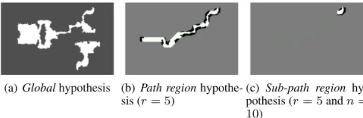
What we call the global hypothesis corresponds to what is most of-ten used for solving a planning problem. It consists of giving the planning algorithm the complete representation of the environment and letting it compute a global solution to the goal from a given source state. So for our tests it corresponds to giving the complete occupancy-grid representation of the environment, and the source and goal position for the robot. The advantage of this hypothesis is that the solutions are global and can thus be globally optimal de-pending on the planning algorithm used. The main disadvantage is that finding a global (optimal) solution is often computationally ex-pensive and thus often slow. Figure 2(a) shows an example of an occupancy-grid representation of a global hypothesis.
5.2.2 Path Region and Sub-Path Region Hypotheses The path region hypothesis supposes a previous path already exists and limits the state space for the planning algorithm in some range around this selected path. The construction of this hypothesis in our tests consists of taking into account only the obstacles around the previous path, considering the rest of the space as obstacles (impass-able). The range is parameterized with r, which for our tests corre-sponds to the number of grid-cells taken into account around the path. The main advantages are: (1) When a solution is found it is a global solution and thus the robot will not get stuck in a local optimum. (2) Often the search is largely sped up, for example in environments such as mazes. One drawback is that it does not take into account that out-side the region the robot did update its environment representation, since the path for the construction of the hypothesis was generated, the environment representation did not change. Once outside the up-dated region, it is likely that the new path in this unchanged environ-ment will converge to the existing path and the same solution will be computed over again consuming time for nothing. A second draw-back is that by only looking for solutions locally around a previous path it can easily discard opportunities that occur during execution (e.g. a door that opens) and thus losing its global optimality. Figure 2(b) shows an example of an occupancy-grid representation of the path region hypothesis with r = 5.
The sub-path region hypothesis is a solution for the first drawback mentioned for the path region hypothesis. Here we take into account only the first part of the existing path that is supposed to change. The last state of this sub-path becomes the sub-goal. The path-region hy-pothesis is constructed for the sub-path and is solved for reaching the sub-goal. Finally, by combining the solution returned by the planning algorithm and the previous solution starting from the sub-goal we re-construct a global path towards the real goal. It has the same range parameter r as the path region hypothesis, and the sub-goal can be expressed with a parameter n s.t. the sub-goal corresponds to the state: f irst state of selected path + n. The main advantage is of course the speed up compared to the path region hypothesis. Figure 2(c) shows an example of an occupancy-grid representation of the sub-path region hypothesis with r = 5 and n = 10.
5.3
Tested Configurations
5.3.1 Instantiations of Plan-Replan
PR-A: This is the simplest configuration. Replanning is only trig-gered when no valid plan is available. The search is done with the A* planner. The only hypothesis used is the global hypothesis.
(a) Global hypothesis (b) Path region hypothe-sis (r = 5)
(c) Sub-path region hy-pothesis (r = 5 and n = 10)
Figure 2. Occupancy-grid representations of hypotheses. White represents free space, gray occupied space.
PR-D: Similar to PR-A, but the search is done with the D* Lite planner.
5.3.2 Instantiation of Continuous Planning
CP-D: Replanning is triggered each time a new action is launched. The hypothesis and planner are the same as for PR-D.
5.3.3 Instantiations of Continuous Proactive Planning with Multiple (10) Hypotheses
To reduce the mission durations and the number of launched default actions, we tested the following combinations of hypotheses. Each of them, in order to instantiate the additional hypotheses, supposes some minimal semantic information is available about where obsta-cles can appear. (For our tests this information was directly available from the simulations, but for a real application it should be provided by another component of the system.)
CPP-1: This configuration uses 10 hypotheses. Each time a “nor-mal” action is launched, it first tries to solve the global hypothesis just like the continuous planning strategy. Then, while there is time left until the action finishes, it sequentially plans for sub-path region hypotheses with A*. Each sub-path region hypothesis has a range parameter r = 5, but the sub-goal parameter n takes respectively the values 2 to 10. Here semantic knowledge is used to select the sub-goals s.t. they correspond to the positions on the previous path just after the places where dynamic obstacles can appear. These hypothe-ses are trying to locally optimize the path to the selected sub-goals with the freshest information available, but without considering that dynamic obstacles can appear or disappear. When an action of the de-fault behavior is launched instead of a “normal” action, it only tries to solve the global hypothesis.
CPP-2: This is almost the same as CPP-1, but for the sub-path regionhypotheses we also add a (hypothetical) obstacle in the cor-responding occupancy-grid on the selected path just before the sub-goals. These hypotheses are thus anticipating the apparition of dy-namic obstacles on the followed path, but without taking into account that obstacles can also disappear. Here even more semantic knowl-edge is used to predict the positions and sizes of future obstacles.
CPP-3: This final configuration has the same principle of CPP-2, i.e. it tries to anticipate the apparition of dynamic obstacles on the followed path (still without taking into account that obstacles can also disappear). But as D* Lite can repair a plan fast for a global hypothesis, all hypotheses are global, where for the last 9 hypotheses a predicted obstacle is taken into account just like for CPP-2.
5.4
Realized Missions and Results
We selected 6 missions from the benchmarks [18]. For each mission a different map (about 512 ∗ 512 grid-cells) was selected from differ-ent categories (dao, wc3maps, rooms, mazes, random (10%), random (40%)). Each mission was realized 30 times with each configuration, and for each Pobstacle∈ {0.2, 0.5, 0.8} to simulate different
dynam-ics.
Most of the time, when a “normal” action was launched, the tested configurations for the continuous proactive planning with multiple hypotheses(CPP-1, CPP-2 and CPP-3) were able to finish the search for the 10 hypotheses in time (before the action finished).
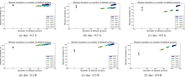
Figure 1 shows the maps from the different categories. Figure 3 shows the results for the tests realized in the environment based on the map of “dao”. The results for the tests realized in the environ-ments based on the five first maps had the same characteristics and can thus be observed in Fig. 3. Figure 4 shows the results for the tests realized in the sixth environment based on the map of “random (40% filled)”.
5.4.1 Case A: the duration of a ”default” action equals the duration needed to plan
We can observe that PR-A and PR-D need to replan about the same number of times, and thus launched about the same number of “de-fault” actions, as expected. As it takes more time for PR-A to replan from scratch than for PR-D to repair the previous plan, the durations of the “default” actions are more important for PR-A than for PR-D, leading to higher total mission durations for PR-A.
CP-D tries to integrate the observed changes during the execution. As dynamic obstacles are added or removed just before launching a new action it has no time to integrate the last changes that invalidate the followed plan. However, by integrating the changes that occurred just before, the resulting plan can change and potentially avoid obsta-cles that will be added on the currently followed plan. By continually optimizing with the available information it generates shorter plans and has to execute less “default” actions resulting in lower mission durations than PR-D.
CPP-1, whose added hypotheses locally optimize the existing path to the selected sub-goals, generates more plans that slightly diverse in the beginning, but remain close to optimal under static conditions, resulting in less “default” actions and even lower mission durations than CP-D.
CPP-2’s hypotheses also take into account the obstacles than can appear. For the first 5 environments, where local solutions were al-most always possible, it was able to find them, resulting in alal-most no need for default behavior. For the sixth environment (based on random (40% filled)) often no local solution was possible, resulting in less decreasing default behavior. Because these hypotheses don’t take into account that obstacles can also disappear the resulting paths are often slightly sub-optimal, resulting in slightly longer paths ex-ecuted. As replanning is often faster than taking a longer path, and here executing a default action only takes the time needed for replan-ning, the mission duration was not improved compared to CP-D.
CPP-3, which also takes into account the obstacles that can ap-pear but searches globally for solutions, had different results than ex-pected. We thought that this would continue to improve the mission durations by finding shorter paths, but we observed that it was actu-ally the configuration that executed the most “normal” actions, result-ing in longer executed trajectories to reach the goal. This is probably because it often found solutions that diverged globally, changing
rad-(a) dao : 0.2 A (b) dao : 0.5 A (c) dao : 0.8 A
(d) dao : 0.2 B (e) dao : 0.5 B (f) dao : 0.8 B
Figure 3. The mission durations against the number of default actions that were executed during the missions, realized in the environment “dao”. Above : without minimum duration for the default actions (indicated with the suffix “A”); Under : with minimum duration of 0.5 seconds for the default actions (indicated with the suffix “B”). From left to right : Pobstacle= 0.2, 0.5, 0.8 (indicated with 0.2, 0.5 or 0.8).
(a) random 40% : 0.2 A (b) random 40% : 0.5 A (c) random 40% : 0.8 A
(d) random 40% : 0.2 B (e) random 40% : 0.5 B (f) random 40% : 0.8 B
Figure 4. The mission durations against the number of default actions that were executed during the missions, realized in the environment “random (40% filled)”. Above : without minimum duration for the default actions (indicated with the suffix “A”); Under : with minimum duration of 0.5 seconds for the default actions (indicated with the suffix “B”). From left to right : Pobstacle= 0.2, 0.5, 0.8 (indicated with 0.2, 0.5 or 0.8).
ically the followed plan, and when obstacles were removed or new obstacles added it doubled back. This was catastrophic for the sixth environment with the highest dynamics (Pobstacle = 0.8), where it
doubled back so often that it barely progressed to the goal. For this setting we showed only the fastest execution of CPP-3 on the graph, the others could even take over 10 hours. CPP-1 and CPP-2 suffered much less from this phenomenon because their hypotheses “stabi-lized” the updated path around the previous path, and when this was not possible they replanned with the latest changes updated.
5.4.2 Case B: a “default” action has a minimum duration of0.5s
As PR-A was able to replan from scratch in less than 0.5s, the per-formances of PR-A and PR-D are about the same.
The improvements of CP-D and CPP-1 w.r.t PR-A and PR-D are emphasized.
The reduction of default behavior realized with CPP-2 made it the fastest for the first five environments, and for the sixth close to the fastest.
The reduction of default behavior realized with CPP-3 made it the second fastest for the first five environments. For the sixth, due to the phenomenon explained before, for low dynamics (Pobstacle =
0.2) the mission durations were about the same as for CP-D, for Pobstacle = 0.5 they were about the same as for PR-A and PR-D,
and for high dynamics (Pobstacle= 0.8) it was catastrophic.
What we can conclude is that proactive planning with multiple hypothesesmay be capable to improve the performances compared to commonly used strategies. As proof of concept, for our tests: If the priority is to complete the mission in minimum time, CPP-1 per-formed the best if the duration of a “default” action equals the dura-tion needed to replan; or CPP-2 if a “default” acdura-tion has a minimum duration of 0.5s. If instead the priority is to avoid default behavior, CPP-2 can be preferred for both cases.
6
Discussion
6.1
Optimality concerns
The presented strategy on itself does not restrict or enforce optimality guarantees. The optimality aspects depend more on the instantiated hypotheses, the selected planners to solve for the hypotheses and the function that selects the “best” action to execute depending on the context.
Guaranteeing some optimality for real applications in unpre-dictable environments is not an easy task, and one should also know what such a guarantee really means. For example, (PO)MDP solvers optimize the expected reward (thus return the best policy for infinite executions), but does this really makes a lot of sense for a mission that is executed only once? For our tests, our planners optimized the length of the path to the goal, but they only guarantee to return the shortest path for the static environment description given as input. If the actual environment changes during the execution, the guarantee is lost. That is why we prefer to search for “good” solutions in the sense of feasible, acceptable and appropriate, instead of guaranteed optimal solutions which we don’t know how to define or obtain in our context.
6.2
Critical Aspects
For obtaining a “good” set of solution-plans with the continuous proactive planning with multiple hypothesesstrategy, some aspects are critical:
• Obviously, the choice and construction of the hypotheses to plan for are very important. We observed that the construction of inter-esting hypotheses is very difficult without enough semantic infor-mation on the environment.
• The planning algorithm selected to solve for a hypothesis must be efficient enough to return a solution before the hypothesis be-comes obsolete.
• If local solutions are admitted for some hypotheses it must be taken into account when selecting the actions to execute. Other-wise it is possible to get stuck in a local optimum.
6.3
Computational Overhead
One can be concerned about the computational overhead because, of course, solving for multiple hypotheses is more computational inten-sive than solving for one hypothesis. For the use cases we consider there is actually no concern because the planning is done during the execution of actions when computational resource is available. How-ever, if one must also minimize the consumption of the CPU, the underlying function that indicates if there is a “hypothesis left to ex-plore” should take this into account and only return true when appro-priate.
6.4
Semantic Information
While the proactive planning with multiple hypotheses paradigm looks promising and natural for anticipating future situations, we ob-serve that it critically needs semantic information to be efficient.
However, if enough semantic knowledge is available, the robot could largely enhance its capabilities, for example by inferring au-tomatically:
• more interesteing hypotheses, taking into account that a person can let the robot pass, a chair can be moved, some places would better be avoided, etc.;
• which hypothesis to instantiate in which context; • which planner to use for solving a particular hypothesis; • how to create the right input for a planner and a hypothesis; • how to schedule the planning episodes. (e.g.: for hypotheses with
defferent time horizons, priorities, ...)
Therefore, we are investigating tools for acquiring and managing se-mantic information , such as the ones presented in [2, 20, 3].
7
Conclusion
We presented the continuous proactive planning with multiple hy-potheses strategy. Its concept is to proactively plan for multiple hypotheses, during the execution of actions, to generate multiple solution-plans from which an appropriate action can be selected when required. To illustrate the concepts, we developed how it could be used for autonomous navigation in dynamic environments. For this purpose we presented the tests we realized and compared the per-formances to two commonly used strategies. The proactive planning with multiple hypothesesparadigm looks promising and natural for anticipating future situations, but needs enough semantic information
to be efficient. We also argued how integrating more semantic infor-mation could enhance the capabilities of service robots. Therefore we continue our work focusing on how this can be done effectively.
REFERENCES
[1] Sankalp Arora, Sanjiban Choudhury, Daniel Althoff, and Sebastian Scherer, ‘Emergency maneuver library-ensuring safe navigation in par-tially known environments’, in Robotics and Automation (ICRA), 2015 IEEE International Conference on, pp. 6431–6438. IEEE, (2015). [2] Michael Beetz, Ferenc B´alint-Bencz´edi, Nico Blodow, Daniel Nyga,
Thiemo Wiedemeyer, and Zolt´an-Csaba Marton, ‘Robosherlock: Un-structured information processing for robot perception’, in IEEE In-ternational Conference on Robotics and Automation (ICRA), Seattle, Washington, USA, (2015).
[3] Michael Beetz, Lorenz M¨osenlechner, and Moritz Tenorth, ‘Crama cog-nitive robot abstract machine for everyday manipulation in human en-vironments’, in Intelligent Robots and Systems (IROS), 2010 IEEE/RSJ International Conference on, pp. 1012–1017. IEEE, (2010).
[4] Michael Brenner and Bernhard Nebel, ‘Proactive continual planning -- deliberately interleaving planning and execution in dynamic - environ-ments’, Tracts in Advanced Robotics, 76, 65–75, (2012).
[5] Ethan Burns, J. Benton, Wheeler Ruml, Sung Wook Yoon, and Minh Binh Do, ‘Anticipatory on-line planning’, in Proceedings of the Twenty-Second International Conference on Automated Planning and Scheduling, ICAPS 2012, Atibaia, S˜ao Paulo, Brazil, June 25-19, 2012, (2012).
[6] Caroline Ponzoni Carvalho Chanel, Charles Lesire, and Florent Teichteil-K¨onigsbuch, ‘A robotic execution framework for online prob-abilistic (re)planning’, in ICAPS 2014, Portsmouth, NH, USA, (2014). [7] Dave Ferguson, Maxim Likhachev, and Anthony Stentz, ‘A guide to heuristic-based path planning’, in Proceedings of the interna-tional workshop on planning under uncertainty for autonomous sys-tems, international conference on automated planning and scheduling (ICAPS), pp. 9–18, (2005).
[8] Maria Fox, Alfonso Gerevini, Derek Long, and Ivan Serina, ‘Plan sta-bility: Replanning versus plan repair’, in ICAPS 2006, Cumbria, UK, (2006).
[9] Malik Ghallab, Dana Nau, and Paolo Traverso, ‘The actor’s view of au-tomated planning and acting: A position paper’, Artificial Intelligence, 208, 1–17, (2014).
[10] C´esar Guzm´an, Vidal Alc´azar, David Prior, Eva Onaindia, Daniel Bor-rajo, Juan Fdez-Olivares, and Ezequiel Quintero, ‘Pelea: a domain-independent architecture for planning, execution and learning’, in Proc. ICAPS, volume 12, pp. 38–45, (2012).
[11] Peter E Hart, Nils J Nilsson, and Bertram Raphael, ‘A formal basis for the heuristic determination of minimum cost paths’, Systems Science and Cybernetics, IEEE Transactions on, 4(2), 100–107, (1968). [12] Sven Koenig and Maxim Likhachev, ‘Improved fast replanning for
robot navigation in unknown terrain’, in Robotics and Automation, 2002. Proceedings. ICRA’02. IEEE International Conference on, vol-ume 1, pp. 968–975. IEEE, (2002).
[13] David Kortenkamp and Reid Simmons, ‘Robotic systems architec-tures and programming’, in Springer Handbook of Robotics, 187–206, Springer, (2008).
[14] Eitan Marder-Eppstein, Eric Berger, Tully Foote, Brian P. Gerkey, and Kurt Konolige, ‘The office marathon: Robust navigation in an indoor office environment’, in ICRA 2010, Anchorage, AK, USA, (2010). [15] Bhaskara Marthi, ‘Robust navigation execution by planning in belief
space’, in RSS 2012, Sydney, Australia, (2012).
[16] Dana S Nau, Malik Ghallab, and Paolo Traverso, ‘Blended planning and acting: Preliminary approach, research challenges’, in AAAI 2015, Austin, TX, USA, (2015).
[17] Anthony Stentz et al., ‘The focussed d* algorithm for real-time replan-ning.’, in IJCAI, volume 95, pp. 1652–1659, (1995).
[18] N. Sturtevant, ‘Benchmarks for grid-based pathfinding’, Transactions on Computational Intelligence and AI in Games, 4(2), 144 – 148, (2012).
[19] Florent Teichteil-K¨onigsbuch, Charles Lesire, and Guillaume In-fantes, ‘A generic framework for anytime execution-driven planning in robotics’, in ICRA 2011, Shanghai, China, (2011).
[20] Moritz Tenorth and Michael Beetz, ‘Representations for robot knowl-edge in the knowrob framework’, Artificial Intelligence, (2015).
[21] Jur Van Den Berg, Dave Ferguson, and James Kuffner, ‘Anytime path planning and replanning in dynamic environments’, in Robotics and Automation, 2006. ICRA 2006. Proceedings 2006 IEEE International Conference on, pp. 2366–2371. IEEE, (2006).
[22] Sung Wook Yoon, Alan Fern, and Robert Givan, ‘FF-Replan: A base-line for probabilistic planning.’, in ICAPS 2007, Providence, RI, USA, (2007).