Robust Parallel-Gripper Grasp Detection using
Convolutional Neural Networks
Mémoire
Alexandre Gariépy
Maîtrise en informatique - avec mémoire
Maître ès sciences (M. Sc.)
Robust Parallel-Gripper Grasp Detection
using Convolutional Neural Networks
Mémoire
Alexandre Gariépy
Sous la direction de:
Philippe Giguère, directeur de recherche Brahim Chaib-draa, codirecteur de recherche
Résumé
La saisie d’objet est une tâche fondamentale du domaine de la robotique. Des avancées dans ce domaine sont nécessaires au déploiement de robots domestiques ou pour l’automatisation des entrepôts par exemple. Par contre, seulement quelques approches sont capables d’effectuer la détection de points de saisie en temps réel. Dans cet optique, nous présentons une architecture de réseau de neurones à une seule passe nommée Réseau à Transformation Spatiale de Qualité de Saisie, ou encore Grasp Quality Spatial Transformer Network (GQ-STN) en anglais. Se basant sur le Spatial Transformer Network (STN), notre réseau produit non seulement une configuration de saisie mais il produit également une image de profondeur centrée sur cette configuration. Nous connectons notre architecture à un réseau pré-entraîné qui évalue une métrique de robustesse de saisie. Ainsi, nous pouvons entraîner efficacement notre réseau à sa-tisfaire cette métrique de robustesse en utilisant la propagation arrière du gradient provenant du réseau d’évaluation. De plus, ceci nous permet de facilement entraîner le réseau sur des jeux de données contenant peu d’annotations, ce qui est un problème commun en saisie d’objet. Nous proposons également d’utiliser le réseau d’évaluation de robustesse pour comparer diffé-rentes approches, ce qui est plus fiable que la métrique d’évaluation par rectangle, la métrique traditionnelle. Notre GQ-STN est capable de détecter des configurations de saisie robustes sur des images de profondeur de jeu de données Dex-Net 2.0 à une précision de 92.4 % en une seule passe du réseau. Finalement, nous démontrons dans une expérience sur un montage physique que notre méthode peut proposer des configurations de saisie robustes plus souvent que les techniques précédentes par échantillonage aléatoire, tout en étant plus de 60 fois plus rapide.
Abstract
Grasping is a fundamental robotic task needed for the deployment of household robots or fur-thering warehouse automation. However, few approaches are able to perform grasp detection in real time (frame rate). To this effect, we present Grasp Quality Spatial Transformer Net-work (GQ-STN), a one-shot grasp detection netNet-work. Being based on the Spatial Transformer Network (STN), it produces not only a grasp configuration, but also directly outputs a depth image centered at this configuration. By connecting our architecture to an externally-trained grasp robustness evaluation network, we can train efficiently to satisfy a robustness metric via the backpropagation of the gradient emanating from the evaluation network. This removes the difficulty of training detection networks on sparsely annotated databases, a common issue in grasping. We further propose to use this robustness classifier to compare approaches, being more reliable than the traditional rectangle metric. Our GQ-STN is able to detect robust grasps on the depth images of the Dex-Net 2.0 dataset with 92.4 % accuracy in a single pass of the network. We finally demonstrate in a physical benchmark that our method can propose robust grasps more often than previous sampling-based methods, while being more than 60 times faster.
Table des matières
Résumé ii
Abstract iii
Table des matières iv
Liste des tableaux vi
Liste des figures vii
Remerciements ix
Introduction 1
1 Deep Learning 3
1.1 Common architectures . . . 3
1.2 Common vision tasks. . . 7
1.3 Data considerations. . . 11
2 Robot Grasping Learning 13 2.1 General Problem Description . . . 13
2.2 Deep Learning Approaches. . . 14
2.3 Dynamic approaches . . . 25 2.4 Grasping Datasets . . . 27 2.5 Classical Approaches . . . 37 3 Preliminary experiments 41 3.1 Learning rotation . . . 41 3.2 Analysis of GQ-CNN . . . 46 3.3 Conclusion . . . 48
4 GQ-STN: Optimizing One-Shot Grasp Detection based on Robustness Classifier 49 4.1 Objectives . . . 49
4.2 Contributions . . . 50
4.3 Problem Description . . . 51
4.4 GQ-STN Network Architecture . . . 52
Conclusion 63
A Other experiments 65
A.1 Alternative GQ-STN architectures . . . 65 A.2 Simulated test environment . . . 67
Liste des tableaux
1.1 The ResNet architecture . . . 5
2.1 Comparison of deep learning approaches to grasping . . . 23
2.2 Summary of the grasping datasets used in deep learning research . . . 28
4.1 Comparison of one-shot methods on evaluation metrics. . . 59
Liste des figures
1.1 The AlexNet architecture . . . 4
1.2 ResNet blocks. . . 5
1.3 The STN applied to two classification tasks . . . 7
1.4 Localization via classification supervision . . . 10
2.1 The five-dimensional grasp rectangle representation . . . 14
2.2 Dex-Net 2.0 grasping pipeline . . . 17
2.3 Visualization of the MultiGrasp architecture. . . 19
2.4 Grasp probability smoothing of a discretized prediction grid . . . 20
2.5 The belief map grasp representation . . . 21
2.6 Network architecture for dynamic grasping. . . 25
2.7 Overview of the Grasp2Vec approach . . . 26
2.8 The BigBIRD data acquisition setup . . . 31
2.9 Sparse grasp labels of the Dex-Net 2.0 dataset. . . 34
2.10 Dex-Net 2.0 dataset . . . 35
2.11 Flowchart of data collection in simulation . . . 36
2.12 The Barrett hand . . . 37
2.13 Pre-deep-learning grasp detection pipeline . . . 39
3.1 Rotational symmetry in grasp rotation learning . . . 42
3.2 Probability of a good grasp after angle perturbation . . . 43
3.3 Learning to grasp by isolating rotation as an input . . . 44
3.4 Probability of a good grasp relative to the grasp angle. . . 45
3.5 Effect of perturbations of ground truths on GQ-CNN’s output. . . 47
4.1 Overview of our method . . . 50
4.2 Complete GQ-STN architecture . . . 52
4.3 Spatial Transformer Network (STN) block for rotation . . . 54
4.4 Physical benchmark setup . . . 56
4.5 Examples of grasp prediction on the dataset . . . 58
4.6 Examples of grasp prediction in the physical benchmark . . . 62
When in doubt, deep it out. Anonymous
Remerciements
Le dépôt de ce mémoire est la bonne occasion de remercier toutes les personnes ayant contribué de près ou de loin à la réalisation de mes études.
D’abord, je veux remercier mon directeur de recherche, le professeur Philippe Giguère, qui a su me guider pour mener à bien mes travaux de recherche. Merci pour ta présence et pour les voyages en conférence qui m’ont fait apprécier davantage la vie d’étudiant gradué. Je veux également remercier mon co-directeur de recherche, le professeur Brahim Chaib-draa de m’avoir accueilli comme stagiaire à son laboratoire et de m’avoir donné le goût de poursuivre au deuxième cycle. De plus, je tiens à remercier le professeur François Pomerleau qui, même si je n’étais son étudiant, était toujours disponible pour répondre à mes questions.
Je remercie toute l’équipe du Véhicule Autonome Université Laval (VAUL), en particulier Julien Becirovski, d’avoir mis sur pied un projet aussi stimulant m’ayant permis d’ajouter une autre corde à mon arc.
Merci à la coalition d’étudiants du DAMAS, du Norlab et du GRAAL pour la camaraderie du midi et du vendredi soir.
Finalement, je tiens à remercier ma copine Sarah-Jade ainsi que mes parents pour leur présence et leur soutient durant ces dernières années d’étude.
Introduction
Grasping, corresponding to the task of grabbing an object initially resting on a surface with a robotic gripper, is one of the most fundamental problems in robotics. Its importance is due to the pervasiveness of operations required to seize objects in an environment, in order to accomplish a meaningful task. For instance, manufacturing systems often perform pick-and-place, but rely on techniques such as template matching to locate pre-defined grasping points (Mercier et al., 2019). In a more open context such as household assistance, where objects vary in shape and appearance, we are still far from a completely satisfying solution. Indeed, in an automated warehouse, it is often one of the few tasks still performed by hu-mans (Correll et al., 2018).
To perform autonomous grasping, the first step is to take a sensory input, such as an image, and produce a grasp configuration. The arrival of active 3D cameras, like the Microsoft Kinect, enriched the sensing capabilities of robotic systems. One could then use analytical methods (Bohg et al., 2014) to identify grasp locations, but these often assume that we already have a model. They also tend to perform poorly in presence of sensor noise. Instead, recent methods have explored data-driven approaches. Although sparse coding has been used (Trottier, Giguère, and Chaib-draa, 2017), the vast majority of new data-driven grasping approaches employ machine learning, more specifically deep learning (Zhou et al.,2018; Park, Seo, et al., 2018a; Park and Chun, 2018; Chu et al., 2018; D. Chen et al., 2017; Trottier, Giguère, and Chaib-Draa, 2017). A major drawback to this is that deep learning approaches require a significant amount of training data. Currently, grasping training databases based on real data are scant, and generally tailored to specific robotic hardware (Pinto et al.,2016; Levine et al.,2018). Given this issue, others have explored the use of simulated data (Mahler, J. Liang, et al., 2017; Bousmalis et al., 2018).
Similarly to computer vision, data-driven approaches in grasping can be categorized into classification and detection methods. In classification, a network is trained to predict if the sensory input (a cropped and rotated part of the image) corresponds to a successful grasp location. For the detection case, the network outputs directly the best grasp configuration for the whole input image. One issue with classification-based approaches is that they require a search on the input image, in order to find the best grasping location. This search can be
exhaustive, and thus suffers from the curse of dimensionality (Lenz et al.,2015). To speed-up the search, one might use informed proposals (Mahler, J. Liang, et al., 2017; Park and Chun, 2018), in order to focus on the most promising parts of the input image. This tends to make the approach relatively slow, depending on the number of proposals to evaluate.
While heavily inspired by computer vision techniques, training a network for detection in a grasping context is significantly trickier. As opposed to classic vision problems, for which detection targets are well-defined instances of objects in a scene, grasping configurations are continuous. This means that there exist a potentially infinite number of successful grasping configurations. Thus, one cannot exhaustively generate all possible valid grasps in an input image. Another issue is that grasping databases are not providing the absolute best grasping configuration for a given image of an object, but rather a (limited) number of valid grasping configurations.
To this effect, we present in this work our master’s research project which aimed at developing a novel single-shot grasping method based on deep learning. In Chapter1, we present general deep learning concepts. Then, in Chapter 2, we define the grasping problem and present a literature review of deep learning solutions used to tackle this task. We also review datasets commonly used for grasping and provide an overview of approaches prior to deep learning to have a historical perspective on the evolution of the field. Next, in Chapter 3, we present preliminary work that focuses on two specific aspects of grasping. In a first experiment, we show how to isolate the rotational parameter of a grasp point as an input of our neural net-work, aiming to facilitate the learning process. In a second experiment, we study the behavior of a pretrained grasp robustness classifier network, Grasp Quality CNN (GQ-CNN) (Mahler, J. Liang, et al., 2017), to visualize the impact on its output grasp robustness probability. Putting together insight acquired from these experiments, we present in Chapter 4 Grasp Quality Spatial Transformer Network (GQ-STN), a novel one-shot neural network architec-ture for grasping (Gariépy et al., 2019). This architecture has been accepted at the 2019 IEEE/RSJ International Conference on Intelligent Robots and Systems (IROS 2019). Finally, in Chapter A, we describe additional experiments that were not included in the IROS 2019 article, but could spark ideas for future works.
Chapter 1
Deep Learning
The advent of deep learning has changed the computer vision landscape, when Krizhevsky et al. (2012) won the ImageNet competition in 2012 using convolutional neural networks. Since this seminal work, deep learning approaches have been successfully applied to a plethora of domains such as robotic grasping (see Chapter2), natural language processing (NLP) (Vaswani et al., 2017), recommender systems (Cheng et al., 2016), voice synthesis (Oord et al., 2016), image captioning (Xu et al., 2015) and much more.
For sake of brevity, we assume that the reader is familiar with the basic concepts of deep learning such as neurons, activation functions, convolutions, features, etc. This is further motivated by the fact that we do not claim any fundamental contributions to deep learning, but rather use it as a toolbox. We will thus instead concentrate on concepts and architectures that are related to our research. For a more thorough overview of the deep learning field in general and its active research avenues, please refer to Goodfellow et al. (2016).
More precisely, we present here an overview of hand-picked subjects that are either relevant for the grasping task (Chap. 2) or to our research project (Chap. 3 and 4), namely common neural network architectures (Sec. 1.1), common computer vision tasks (Sec. 1.2) and the importance of data in deep learning research (Sec.1.3).
1.1
Common architectures
1.1.1 Alexnet
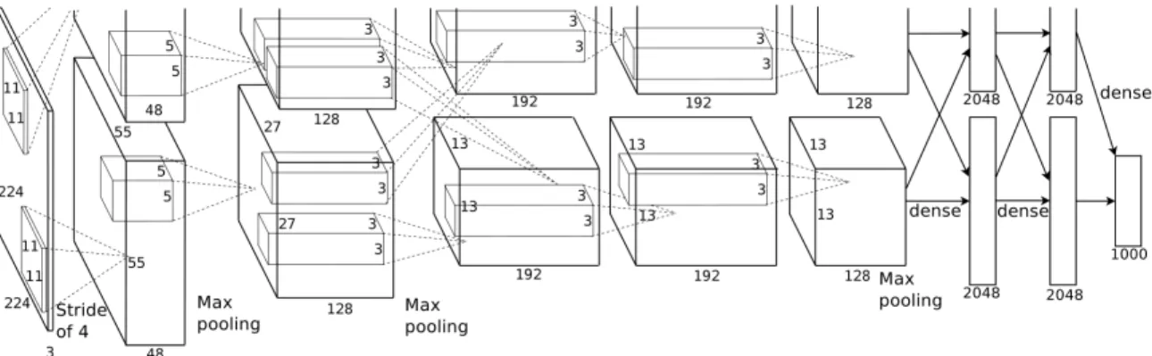
The AlexNet architecture was introduced by Krizhevsky et al. (2012). This architecture had a tremendous impact at the 2012 ImageNet competition (see Section1.2.1) by nearly halving the classification error from the previous year, with a 16.4 % top-5 error (compared to a previous 25.8 %). Notably, it was the first time a deep learning technique was used at this competition. The AlexNet architecture, depicted in Figure 1.1, consists of 8 layers. The first 5 layers are
Figure 1.1 – The AlexNet architecture from (Krizhevsky et al., 2012).
convolutional and the last three are fully-connected. Contrary to previous Convolutional Neu-ral Network (CNN) architectures, AlexNet used the Rectified Linear Unit (ReLU) activation function, which has now become a standard practice. It can be seen in Figure1.1that the net-work is split in two parts. This architectural choice was purely driven by hardware constraints at the time. Indeed, the neural network did not fit the memory of a single Graphical Process-ing Unit (GPU), so two GPU were required durProcess-ing trainProcess-ing. With the rapid advancement of GPUs, modern re-implementations of AlexNet can fit in a single card: see Joseph Redmon and Angelova (2015) for instance.
1.1.2 ResNet
The ResNet architecture was introduced by He et al. (2015a) and won the 2015 ImageNet competition with a 3.57 % top-5 error. Like AlexNet did in 2012, ResNet also reduced by half the error of the previous year, brigning a significant impact to the field. It also reached super-human performance.
The main innovation brought by He et al. (2015a) was the residual connections in the network architecture, as depicted in Figure 1.2. Most previous architectures such as AlexNet had a completely feed-forward structure: a convolutional layer produced a feature map that was an input to only the next layer. However, the basic building block of ResNet contains a skip connection, which simply is a copy of the input feature map x. The skip connection is added to the output of the residual block F (x, Wi), yielding the basic building block:
y = F (x, Wi) + x
In this equation, the output y of a layer is determined by the element-wise addition of a function F (x, Wi) and of its input x (the skip connection). F (x, Wi) here represents the
residual block, made of convolution operations with the learnable parameters Wi.
In their paper, He et al. (2015a) describe two types of residual blocks for ResNet. The first block, the basic building block, consists of two convolutional layers where there is a skip
Figure 1.2 – Residual blocks used in ResNet architecture. (Left) A building block used in ResNet-18 and ResNet-34 architectures. (Right) A bottleneck building block used in deeper architectures (ResNet-50/101/152). Figure from (He et al.,2015a).
Table 1.1 – Table detailing ResNet-18/34/50/101/152 architectures. From (He et al., 2015a).
connection from the input of the feature map to the output of the second convolutional layer. This residual block is used in ResNet-18 and ResNet-34 networks. The author also introduced a second block named the bottleneck block. The bottleneck block consists of three convolutional layers instead of two. The first convolutional layer uses 1 × 1 filters to reduce the size of the input feature-map. Then, a convolutional layer of 3 × 3 filters operates on the reduced feature map. Finally, another layer of 1 × 1 filters restore the feature map to its original size. As for the other residual block, there is a skip connection between the input feature map of the first convolutional layer and the output of the last convolution layer. The goal of the bottleneck block is to reduce the number of parameters of the model as the larger 3 × 3 convolution operates on a smaller feature map. It reduces the memory footprint of deeper models and decreases their training time.
The ResNet architecture consists of an arrangement of building blocks or bottleneck building blocks, depending of the depth of the network. Such arrangements are detailed in Table 1.1 The authors show that, because of the residual connections in its architecture, ResNets tend to train much faster, while converging to more accurate models than networks without residual
connections. The authors argue that it is because a ResNet can more easily learn an identity mapping between the input feature map and the output feature map. Indeed, if all learnable variables of the convolutional layers in the residual blocks are set to zeros, the input and output would be the same because of the skip connection. This is not the case for networks that do not have skip connections, where small changes to the variables can have a big impact on the output. It is the justification given by the authors concerning why they are able to train very deep models up to 1202 layers. With their ResNet architecture, layers in a deep network can still bring small contributions without degradation of the information. In later work, Veit et al. (2016) showed that, because of the skip connections, deep ResNets behave like ensembles of shallower feed-forward networks. They showed that the gradient in ResNets can easily flow layers to layers via the skip connections, enabling deep networks to be trained as easily as shallower ones.
Given their excellent training behavior and overall accuracy, we used ResNets in all of our network architectures. For example, we used them for preliminary experiments in Chapter 3. We also used them for our single-shot detection architectures such as our GQ-STN network and the baseline model, both described in Chapter 4.
1.1.3 Spatial Transformer Network
Jaderberg et al. (2015) introduced the Spatial Transformer Network (STN). It is a drop-in block that can be inserted between two feature maps of a CNN to learn a spatial trans-formation of the input feature map. In some sense, it acts as an attention mechanism, by narrowing/reorienting the feature maps of objects in a more canonical representation for the task at hand. The Spatial Transformer Network (STN) consists of three parts: a localization network, a grid generator and a sampler. The localization network is the part of the STN that contains learnable parameters. It usually consists of a small neural network whose task is to learn a transformation matrix Λ2×3. This matrix is passed to the grid generator that produces a sampling grid in the input feature map. This grid is fed to the sampler that produces the output feature map via an interpolation method such as bilinear sampling. Together, the grid generator and the sampler perform an operation akin to texture mapping. The grid generator and the sampler do not contain any learnable parameters, but are still fully differentiable. This enables end-to-end learning of the localization network parameters jointly with the parameters of the rest of the network.
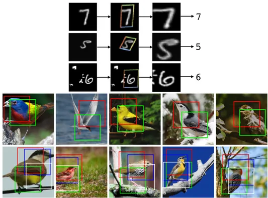
In the paper, the authors show experiments on the distorted MNIST classification dataset, which consists of black and white images of digits that have been translated, cluttered, rotated, scaled and distorted. They show that the STN can properly focus on the distorted digit in the image and transform it so it is centered in a upright manner, facilitating the classification task by the network downstream. The authors also show that using multiple STN in parallel results in a specialization of the STNs. For the task of bird classification on the CUB-200-2011
Figure 1.3 – The STN applied to two classification tasks. (Top) On the distorted MNIST dataset, the STN properly focuses on the digit, facilitating the recognition by the classification network. (Bottom) On the CUB-200-2011 dataset, multiple STNs in parallel learn to focus on different parts of the bird. Figures from (Jaderberg et al.,2015).
dataset, the different STNs focus on different parts of the birds, such as the head, the wings or the body. Both tasks can be seen in Figure 1.3. It is worth mentioning that in both cases, there is absolutely no supervision for the localization network that learns entirely from the classification loss. As we will see in Section 4.4.3, it is also possible to train the localization network in a supervised or semi-supervised manner.
In Section 4.4.1, we show how we used STNs for cascaded geometric transforms of images, in the context of single-shot grasp detection.
1.2
Common vision tasks
In this Section, we describe two basic vision tasks: classification and object detection. These tasks drove the deep vision community forward, generating many innovations. For instance, the AlexNet (Section 1.1.1) and ResNet (Section 1.1.2) both were invented for the image classification task. Both tasks are also present in the context of perception for grasping. In Section 2.2, we will thus present approaches that are derived from both classification and object detection methods coming from the field of computer vision.
1.2.1 Classification Task
In its simplest form, the classification task consists in determining which object class is de-picted among a closed set of possible classes, given an RGB image. The apparition of the ImageNet dataset (Deng et al.,2009) and the ImageNet Large Scale Visual Recognition Com-petition (ILSVRC) (Russakovsky et al., 2014) are responsible for driving forward research to superhuman performance (He et al.,2015b; He et al.,2015a). The ImageNet dataset is further discussed in Section 1.3.
Modern classification networks consist of two main parts: a feature extractor and a classifica-tion head. The feature extractor turns the input image into a tensor representaclassifica-tion named the visual embedding. The feature extractor is usually a convolutional neural network (Krizhevsky et al., 2012; He et al., 2015a; Szegedy et al., 2016). Then, the classification head is used to determine which class is present in the image, given the visual embedding. Early work such as Krizhevsky et al. (2012) and Simonyan et al. (2015) used three fully-connected layers after the convolutional layers of the feature extractor. Nowadays, since networks are becoming deeper and deeper, the classification heads are becoming simpler, transferring the representational power to the feature extractor. For instance, both He et al. (2015a) and Szegedy et al. (2016) have a single fully-connected layer as classification head. The classification head outputs a vec-tor that has a length equal to the cardinality of the set of classes. It represents (unnormalized) probabilities of each class being present in the image.
1.2.2 Detection Task
The detection task consists in finding both the location and the class of object instances in an image. Contrary to the classification task, there can be multiple objects present in the image. The Pascal Visual Object Classes (VOC) dataset and the Microsoft Common Object in Context (MS-COCO) (Lin et al., 2014) dataset are two examples of commonly-used object detection datasets. Multiple approaches for object detection have been put forward over the years. However, this section is not meant as an exhaustive review of deep learning based object detection approaches. We will instead concentrate on a few approaches that were influential for grasping based on deep learning (Section 2.2). For a review on object detection, see Zhao et al., 2019.
S. Ren et al. (2015) proposed a two-stage network architecture named Faster R-CNN. A first convolutional network, named Region Proposal Network (RPN), is slid over the input image. In this grid-search process, the RPN is responsible for generating bounding box proposals, by predicting the offsets for both size and position of predetermined anchor boxes. It also predicts a score representing the probability of each bounding box of containing an object. Then, for each bounding box proposal, a second network named Fast R-CNN (Girshick, 2015) determines the class of the object. Both RPN and Fast R-CNN are trained independently. In
the paper, the authors explored ways to share parameters between the two networks, but this was found to be non-trivial, as their proposed method is meant as a two-step process.
Joseph Redmon, Divvala, et al. (2015) introduced the You Only Look Once (YOLO) architec-ture. Contrary to Faster R-CNN, YOLO used a single-network for both bounding box proposal and object classification. It also used an AlexNet feature extractor. Interestingly, YOLO is a successor of “Real-Time Grasp Detection Using Convolutional Neural Networks” (Joseph Red-mon and Angelova,2015), presented in Chapter2. The main idea behind YOLO is to output a vector of 1470 elements via fully connected layers at the end of the AlexNet feature extractor. This vector is interpreted as a cell grid of 7 × 7, with a prediction vector of dimension 30 for each cell. These correspond to two bounding box predictions, whose centers are located inside the cell. Each bounding box consists of 4 spatial parameters (x, y, width, height) and the probability O of the bounding box containing any object. At each cell, there is also a pre-diction of P (Classi|O) for each of the 20 classes of the Pascal VOC dataset. YOLO performs
as well as Faster R-CNN while being 90 times faster.
In a latter version of their work, J. Redmon et al.,2017improved their YOLO architecture: the YOLOv2 architecture. Among other improvements, the authors replaced the fully-connected layers by a convolutional layer, resulting in an Fully Convolutional Network (FCNN) architec-ture. Given the output volume of the feature extractor of size 13 × 13 × 1024, a convolution of 301 1 × 1 filters is used to obtain the prediction grid. This FCNN architecture yields several advantages. First, because the output grid is obtained via convolution, the receptive field of each cell in the output grid is restricted to a more relevant part of the input image. This is not the case for YOLOv1, where each grid cell has access to features of the whole image, due to the fully-connected layers. Second, being fully convolutional, YOLOv2 can adapt to multiple input image sizes. At training time, the authors even propose to resize images to be robust to multi-scale prediction.
1.2.3 Comparison of classification and detection tasks
The classification and the detection tasks are closely related. Visual features that are relevant for a classification task (e.g. Is this a cat? ) tend also to be useful for a detection task (e.g. Is there a cat in the image? Where? ). Therefore, it is common practice to use a classification network pre-trained on ImageNet, replace the classification head by a detection head and then fine-tune everything together (S. Ren et al., 2015; Joseph Redmon, Divvala, et al., 2015; J. Redmon et al., 2017).
Apart from fine-tuning, the close proximity between classification and detection have been directly exploited in practice. A prime example is the Spatial Transformer Network (STN) presented in Section 1.1.3. The localization network, as seen in Figure1.3, learns to focus on
1. In fact, YOLOv2 predicts 5 bounding boxes per cell instead of two in the original YOLO architecture, resulting in 45 outputs per cell.
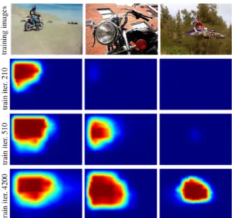
Figure 1.4 – Probability heat-maps of the presence of a motorbike in the image. The network is trained without any localization label, having only a list of objects present in the image. Figure from Oquab et al., 2015.
specific parts of the image, which can be interpreted as an attention mechanism that performs unsupervised detection via a classification gradient signal.
Another example is the article “Is object localization for free?-weakly-supervised learning with convolutional neural networks” (Oquab et al., 2015), in which the authors proposed to use a network trained only on the classification task to perform object detection. The only label used for training is a list of objects present in the image, without any information on their actual location. Similarly to YOLOv2, the authors replaced the fully-connected layers by convolutions. As an effect, instead of outputting a fixed 1 × 1 × K vector, where K is the number of classes, the network outputted a tensor T of dimension n × m × K, where n and m depends on the size of the input image. The final 1×1×K classification vector can be retrieved via global max-pooling2. Their key observation was that, at training time, the propagation of
the gradient through the max-pooling operation gives a good indication of where an object is located. Because of the global max-pooling operation, only the best location in the n × m grid for each class is used, and gradient is only propagated through this element, giving away the location of the object via its receptive field. Figure 1.4shows the probability heat-maps of a motorbike being present by projecting each probability of T corresponding to the motorbike class to its receptive field.
This close relationship between the classification task and the detection task serves as an intuition for our work. Indeed, in Chapter 4, we show how to use the gradient of a grasp robustness classification network to guide the training of a one-shot grasp detection network.
1.3
Data considerations
Data is at the heart of any deep learning application. To tackle hard tasks that lie in a high-dimensional input space such as image classification or object detection, models with a high capacity are typically required. However, a large capacity model is inclined to over-fitting, if not regularized properly. The most natural way of regularizing a machine learning model is to acquire more data for the training set.
Success and good generalization of methods thus rely on the availability in great quantities of good quality data. Recent successes in image classification are in great part due to the availability of such large datasets. For instance, the ImageNet dataset contains around 14 million annotated images. In comparison, Caltech-256 (Griffin et al., 2007), which is an older image classification dataset, contained only 30k images.
Data from the ImageNet dataset comes from search engine queries of the category name, its synonyms and its translation in other languages. To ensure the good quality of the labels, all images were verified by multiple humans on Amazon’s Mechanical Turk (Buhrmester et al., 2011)3. A similar data annotation scheme has been used by Lin et al.,2014for the MS-COCO
dataset (328k images). These two examples demonstrate that the manual annotation of large scale datasets is feasible but is, however, an expensive process both time-wise and cost-wise. On the other hand, manual annotations are impractical for some complex tasks. A good example is the 6 degrees of freedom (DoF) pose detection task (Hinterstoisser et al.,2019). The annotation process consists in determining which known objects are in a scene and to estimate their pose, e.g. x, y, z, yaw, pitch, roll. Even with specialized tools, this takes considerably longer than annotating a classification dataset. Hinterstoisser et al., 2019 estimated it takes around 7 minutes per image. At this rate, gathering a dataset of the size of ImageNet would require around 1.6M man-hours (186 man-years). This problem regarding the data cost is particularly prevalent in robotics, where the input domain is of high dimensionality.
To circumvent this problem, employing simulation for dataset acquisition is an attractive al-ternative. In simulation, the environment is completely controlled and the 6 DoF annotation process can be automated, dramatically reducing the cost of data. Also, the full observability of the world can be a desirable property for reinforcement learning, where complex reward functions can be derived from the world state. Simulation is used for many grasping datasets, as presented in Section 2.4. However, simulation suffers from what is called the reality gap problem. The reality gap problem arises when a model learned in simulation does not gener-alize well to real world conditions. This is due to the fact that many aspects of the real world are difficult to simulate accurately, e.g. producing photo-realistic images for vision (Depierre et al., 2018), modelling sensors noise (Mallick et al., 2014) or predicting noisy actuation.
3. Amazon’s Mechanical Turk is a system that allows the outsourcing of the data annotation process to distributed users around the world.
A variety of approaches exist to tackle this reality gap problem. First, there is domain random-ization (X. Ren et al.,2019; Tobin et al.,2018; Bousmalis et al.,2018). It consists of adding a large variety to the simulation, for example by randomizing textures and lighting. The aim is that the real world will simply look like another variation of the simulation. Another approach is domain adaptation. Mercier et al., 2019proposed to include a Multi-Adversarial Domain Adaptation (MADA) (Pei et al.,2018) module to their pose estimation network. This module prohibited the learning of features that are specific to one of the two domains (simulation and real world). The message here is that learning in simulation is feasible, though one needs to address the reality gap problem to ensure good generalization.
Chapter 2
Robot Grasping Learning
In this chapter, we provide an overview of state-of-the-art grasping research. First, in Sec-tion 2.1, we formulate a general problem description for grasping. Second, in Section 2.2, we classify deep learning approaches for grasp detection, which are approaches that use a neural network to find the best grasp configuration. Then, in Section 2.3, we present dynamic ap-proaches where, instead of learning to find a grasp configuration, an agent learns a policy to control the joints of a robotic arm directly. Thereafter, Section 2.4 enumerates the common grasping datasets seen in deep learning literature. Finally, in Section2.5, we take a step back and look at classical approaches that paved the way to today’s research, taking a critical look at previous methods to highlight ideas that are still relevant today.
2.1
General Problem Description
In the context of deep learning research, grasp detection is closely related to the object de-tection problem (see Section 1.2.2). However, grasp detection lies in a bigger dimensionality prediction space than object detection because, compared to object detection, we must make additional predictions, including at least the orientation of the gripper. Also, because grasp configurations are continuous, there is potentially an infinite number of positive grasps in a scene. This means that, even if grasping borrows from object detection, we must develop a specific problem formulation for the grasping task.
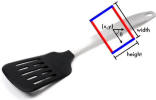
The most used grasp representation is the grasp rectangle (Jiang et al., 2011), depicted in Figure 2.1. A grasp rectangle consists of a 2D coordinate x, y, a width w, a height h and an angle θ on the XY plane. The width represents the opening of a parallel gripper, while the height delimits the bounding box of the two fingers.
To evaluate a grasp rectangle, one can compute the Jaccard index (or Intersection-over-Union) to the closest ground truth. Given a prediction A and a ground truth B, the Jaccard index
Figure 2.1 – The five-dimensional grasp rectangle representation. It represents a grasp in 2D from the top view. Figure from Joseph Redmon and Angelova (2015)
J (A, B) is given by:
J (A, B) = |A ∩ B|
|A ∪ B|. (2.1)
A grasp is considered positive if the Jaccard index is more than 25 % and if the angle of the prediction is within 30◦ of the ground truth. As we will see later in Chapter4, this metric is problematic because it lies in the image space and has no connection to the actual physical grasp robustness.
The grasp rectangle is a simplification of the full 3D, 7-dimensional configuration of a parallel gripper (x, y, z, yaw, pitch, roll, opening). Jiang et al. argue that the rectangle representation works well in practice and is much simpler computationally, reducing significantly the search space of grasp candidates. Still, some recent work operates in the full 7-dimensional space, where they find the best grasping pose in full 3D grasp configuration depth images or point clouds (Pas et al., 2017; H. Liang et al.,2018; Schmidt et al., 2018).
Another grasp representation commonly seen in the literature is the point representation (Sax-ena et al., 2008). A grasp is considered simply as a x, y coordinate in an image. To evaluate a prediction, one verifies if its distance to the closest ground truth is under a certain threshold. This representation has a number of limitations. For instance, it does not take into account neither the orientation nor the size of grasping points. Moreover, it tends to over-estimate the performance of grasping algorithms; See Jiang et al. (2011) for a detailed analysis.
2.2
Deep Learning Approaches
Over the years, many network architectures have been proposed to solve the grasping problem. In this section, we grouped these architecture by themes, either based on their overall method of operation or on the type of generated output. Section 2.2.1 describes ranking approaches, where deep learning techniques are used to rank different grasp candidates. Section 2.2.2 presents one-shot approaches where the top grasp is directly obtained from sensory data,
i.e. without intermediary steps. One-shot approaches are further classified into four main categories: regression approaches, multibox approaches, anchor-box approaches and discrete approaches. Table 2.1summarizes the most important approaches.
2.2.1 Proposal + Classification Approaches
Drawing inspiration from previous data-driven grasping methods (Bohg et al., 2014), some approaches work in a two-stage manner. They first propose grasp candidates then choose the best one via a classification score. Note that this section does not include architectures employing Region Proposal Network (RPN), as these are applied on a fixed-grid pattern, and can be trained end-to-end. They are discussed later.
Early work in applying deep learning on the grasping problem employed such a classification approach. For instance, Lenz et al. (2015) used a cascade of two fully-connected neural net-works. The first one was designed to be small and fast to evaluate and perform the exhaustive search. The second and larger network then evaluated the best 100 proposals of the previous network. This architecture achieved 93.7 % accuracy on the Cornell Grasping Dataset (CGD) (see Section 2.4.1).
Pinto et al. (2016) reduced the search space of grasp proposals by only sampling grasp locations x, y and cropping a patch of the image around this location. To find the grasp angle, the author proposed to have 18 outputs, separating the angle prediction into 18 discrete angles by 10◦ increments. In subsequent work, Gupta et al. (2018) argued that to use grasping in a low-cost setting, modelling noise is a necessary step in grasp point detection. This is due to the fact that data gathered using a low-cost robot is very noisy because of imperfect execution and calibration errors. They thus proposed to collect data with multiple inaccurate robots and to use this noisy data for training. For grasp prediction, they used the same method as in their previous work (Pinto et al., 2016). However, they introduced the Noise Modelling Network (NMN) that learns a marginalization operator over the grasp probabilities, given i) a visual embedding of the scene, ii) the identifier of the robot that collected the data identifier and iii) the grasp location in image space. In other words, the NMN re-weighted probabilities of the grasp outcomes, therefore learning that some grasps were more difficult to execute on certain robots than others. The author reported an improvement of 43.7 % compared to a model trained in a controlled lab environment without noise modelling.
The EnsembleNet Asif et al. (2018) worked in a radically different manner. It trained four distinct networks to propose different grasp representations (regression grasp, joint regression-classification grasp, segmentation grasp, and heuristic grasp). Each of these proposals was then ranked by the SelectNet, a grasp robustness predictor trained on grasp rectangles. Their model is 2-5 % more accurate than the separate CNN models it aggregates.
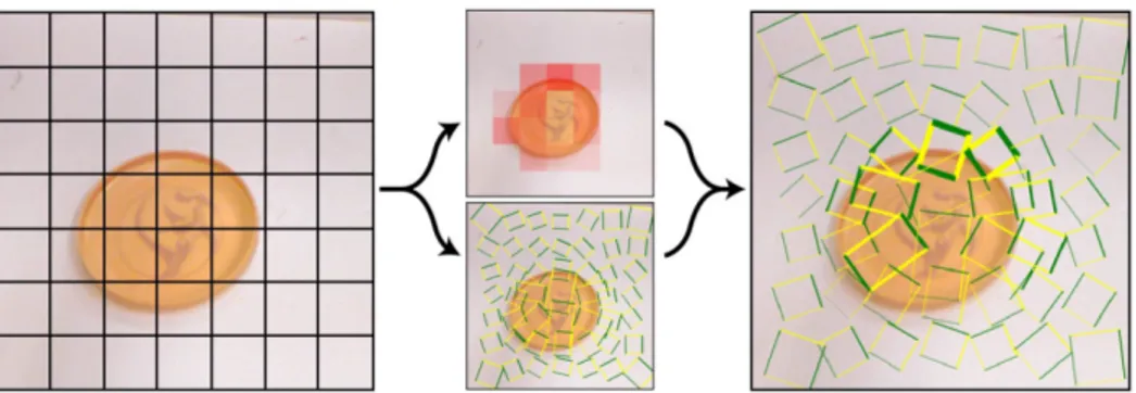
(2017) relied entirely on a simulator setup to generate a large database of grasp examples called Dex-Net 2.0 (see Section 2.4.2). Each grasp example was rated using a rule-based grasp robustness metric named Robust Ferrari Canny. By thresholding this metric, they trained a deep neural network, dubbed Grasp-Quality CNN (GQ-CNN), to predict grasp success or failure. The GQ-CNN takes as input a 32 × 32 depth image centered on the grasp point, taken from a top view to reduce the dimensionality of the grasp prediction. Note that this simplification is used by others, notably Levine et al. (2018). For grasp detection in a depth image, they used an antipodal sampling strategy. This way, 1000 antipodal points on the object surface are proposed and ranked with GQ-CNN. An overview of the method is presented in Figure 2.2. Even though their system is mostly trained using synthetic data, it performed well in a real-world setting. For example, it achieved a 93 % success rate on objects seen during the training time and 80 % success rate on novel objects on a physical benchmark. Furthermore, using a CNN instead of point-cloud matching, it was three times faster than their previous work Dex-Net 1.0 (Mahler, Pokorny, et al., 2016). They also report better generalization on novel objects. In the later Dex-Net 3.0 (Mahler, Matl, Liu, et al.,2018),the authors used GQ-CNN to learn the robustness of suction grasps instead of parallel gripper grasps. In Mahler and Goldberg (2017) and Mahler, Matl, Vishal Satish, et al. (2019), the authors extended Dex-Net 2.0 and Dex-Net 3.0 for bin-picking tasks.
Park and Chun (2018) decomposed the search for grasps in different steps, using STNs. The first STN acted as a proposal mechanism, by selecting 4 crops as candidate grasp locations in the image. Then, each of these 4 crops were fed into a single network, comprising a cascade of two STNs: one estimated the grasp angle and the last STN chose the image’s scaling factor and crop. The latter crop can be seen as a fine adjustment of the grasping location. The four final images were then independently fed to a classifier, to find the best one. Each component, being the STNs and the classifier, were trained on CGD separately using ground truth data and then fine-tuned together. This is a major distinction from other Proposal + Classification approaches, as the others cannot jointly train the proposal and classification sub-systems. The author reported an accuracy of 89.6 % on the CGD. Note that this approach bears some similarity to our Grasp Quality Spatial Transformer Network (GQ-STN) approach presented in Chapter4, as they both make use of STNs. However, our approach was developed independently and is not a successor of Park and Chun (2018).
Instead of learning top-view grasping configurations, Pas et al. (2017) trained a network to learn to score directly a full 6-degrees-of-freedom grasps on point clouds. To do so, they projected the voxelized point cloud from the point of view of the gripper into a rasterized depth image. Grasp candidates came from random sampling. The author sampled a random point and determined a local normal coordinate frame using principal component analysis (PCA) of the neighboring points. They then performed a grid search in this local frame to find grasps that do not intersect with the point cloud but contain points between the fingers.
Figure 2.2 – (Top) Dex-Net 2.0 grasping pipeline. Antipodal grasp candidates are sampled and evaluated by the Grasp-Quality CNN (GQ-CNN). The best candidate is executed. (Bottom) Full Architecture of GQ-CNN. Figures from Mahler, J. Liang, et al. (2017).
In a similar manner, H. Liang et al. (2018) evaluated the quality of grasps directly in the 3D point clouds, instead of depth images, using an architecture similar to PointNet (Qi et al., 2016). They generated ground truth annotation on YCB meshes (see Section 2.4.1) using force-closure and grasp wrench space as grasp quality metrics to train their network.
Some work used tactile modalities to improve ranking approaches. Calandra, Owens, Upad-hyaya, et al. (2017) integrated tactile data from GelSight sensors and RGB images as inputs to a CNN. They showed that it enables better precision of grasp success prediction compared to having only RGB images or depth images. Calandra, Owens, Jayaraman, et al. (2018) went further by using tactile grasp information to learn a grasp adjustment, in order to go from a negative grasp to a positive one. A similar re-grasping strategy is presented in Hogan et al. (2018).
Kappler et al. (2016) presented more theoretical work on ranking approaches. Usually, grasp models are trained in a binary fashion: a grasp configuration is either positive or negative. From this point of view, grasping is treated as a two-class classification problem. The authors argued that, to have a better decision boundary, we should encode the loss function as an explicit ranking problem. They showed how to train this ranking loss with data that has only binary success labels. They reported significant improvement of their method over binary classification loss, out-performing it 84 % to 41 % for large objects of the Cornell Grasping Dataset.
2.2.2 One-Shot Approaches
This section contains an overview of one-shot detection approaches in grasping. These ap-proaches can predict directly the best grasp configuration in a scene, without relying on an intermediary candidate proposal step. The main advantage is that a single inference is re-quired, dramatically reducing computation time. Work done on one-shot grasp detection is often influenced by the state-of-the-art in object detection. For more details on this task, see Section 1.2.2. We subdivide single-shot approaches in four categories, which are presented below.
Regression Approaches
To eliminate the need to perform the exhaustive search of grasp configurations, Joseph Redmon and Angelova (2015) presented the first one-shot detection approach. To this effect, the authors proposed different CNN architectures, in which they always used an AlexNet (Krizhevsky et al., 2012) pretrained on ImageNet as the feature extractor. To exploit depth, they fed the depth channel from the RGB-D images into the blue color channel, and finalized training by fine-tuning. The first architecture, named Direct Regression, directly regressed from the input image the best grasp rectangle represented by the tuple {x, y, width, height, θ}. The second architecture, Regression + Classification added object class prediction to test its regularization effect. The author achieved an accuracy of 84.4 % and 85.5 % for respectively Direct Regression and Regression + Classification. Being early work on one-shot grasp detection on the Cornell Grasping Dataset, Joseph Redmon and Angelova’s article brought valuable insight. They showed how to leverage a network pre-trained on ImageNet (3 color channels) for their RGB-D images (4 channels), by simply replacing the blue channel of the RGB input by the RGB-D (depth) channel. Another insight was that the grasp angle of the rectangle representation is two-fold rotationally symmetric; a grasp rectangle and its rotation by 180 degrees are totally equivalent. The authors thus proposed to encode the angle prediction θ as two outputs: sin 2θ and cos 2θ.
Kumra et al. (2017) further developed the Direct Grasp architecture for one-shot detection, by employing the more powerful ResNet-50 architecture (He et al., 2015a). They also explored
a different strategy to integrate the depth modality, while seeking to preserve the benefits of ImageNet pre-training. As a solution, they introduced the multi-modal grasp architecture which separated RGB processing and depth processing into two different ResNet-50 networks, both pre-trained on ImageNet. Their architecture then performed late fusion, before the fully connected layers performed direct grasp regression. They reported a score of 89.21 % on CGD. Even though most work on one-shot grasp detection uses a top-view simplification of the grasp-ing problem, Schmidt et al. (2018) developed a DNN architecture for 6-degrees-of-freedom grasping. Their network outputted a grasping point x, yz, roll, pitch, yaw relative to the po-sition of a depth camera. Using an off-the-shelf planner, they generated a dataset using YCB and KIT objects, which comprises 3D scans of real objects (see Section 2.4.1), and trained in simulation. The article also presents experiments on a real-world ARMAR-III robot.
Multibox Approaches
Joseph Redmon and Angelova (2015) also proposed a third architecture, MultiGrasp, separat-ing the image into a regular grid (dubbed Multi-box). At each grid cell, the network predicted the best grasping rectangle, as well as the probability of this grasp being positive. The grasp rectangle with the highest probability was then chosen. Separating the image into such a grid makes it easier to learn to grasp circular objects, for instance a Frisbee. A key problem of the Direct Regression approach is that the network tends to converge to the mean of all grasp locations, which is the center of the object, clearly an invalid grasping point. The MultiGrasp architecture achieved 88.0 %, which is 3.6 % better that Direct Grasp. A visualization of MultiGrasp can be seen in Figure 2.3. Trottier, Giguère, and Chaib-Draa (2017) improved results with a similar approach but by employing a custom ResNet architecture for feature extraction. The authors reported accuracy of 89.15 % on CGD. They also cited the reduced need for pre-training on ImageNet.
Figure 2.3 – Visualization of the MultiGrasp architecture. Predictions are made on a regu-lar grid, where the network predicts at each cell the best grasping rectangle as well as the probability of this grasp being positive. Figure from Joseph Redmon and Angelova (2015). L. Chen et al. (2019) remarked that grasp annotations in grasping datasets are not exhaustive. Consequently, they developed a method to transform a series of discrete grasp rectangles to
a continuous grasp path. Instead of matching a prediction to the closest ground truth to compute the loss function, they mapped the prediction to the closest grasp path. This means that a prediction that falls directly between two annotated ground truths can still have a low loss value, thus (partially) circumventing the limitations of the Intersection-over-Union (IoU) metric when used with sparse annotation, as long as the training dataset is sufficiently densely labeled (see Figure2.9). The authors re-used the MultiGrasp architecture from Joseph Redmon and Angelova for their experimentation.
Anchor-box Approaches
Zhou et al. (2018) introduced the notion of oriented anchor-box, inspired by YOLO9000 (J. Redmon et al.,2017). This approach is similar to MultiGrasp (as the family of YOLO object detectors is a direct descendant of MultiGrasp (Joseph Redmon and Angelova, 2015)) with the key difference of predicting offsets to predefined anchor boxes for each grid cell, instead of directly predicting the best grasp at each cell. The authors reported a performance of 97.74 % on the CGD. A similar anchor-box approach is presented in Park, Seo, et al. (2018a). Chu et al. (2018) extended MultiGrasp to multiple objects grasp detection by using region-of-interest pooling layers (S. Ren et al.,2015). A similar architecture is presented in Zhang et al. (2018), where the authors also present experiments with overlapping objects.
Park, Seo, et al. (2018b) exposed the fundamental issue of rotation invariance in grasping, arguing that geometric transformations of the input image is harmful on the performance of deep-learning-based grasping methods. They thus introduced the rotation ensemble module (REM), which is a block inserted at the end of a YOLO9000 (J. Redmon et al.,2017) detection architecture, before the final prediction layers. They achieved 97.6 % on the CGD.
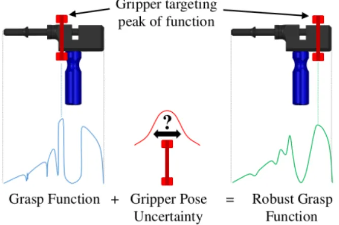
Figure 2.4 – Smoothing grasp scores obtained by evaluating a scoring function on a regular grid. Due to gripper localization uncertainty, the grasp position having the highest score (left) might not be the most appropriate, after incorporating robot uncertainty (right). Figure from Johns et al. (2016).
Discrete Approaches
Johns et al. (2016) proposed to use a discretization of the space with a granularity of 1 cm and 30◦. In a single pass of the network, the model predicts a score at each grid location. Their method can explicitly account for gripper pose uncertainty. Indeed, if a grasp configuration has a high score, but the neighboring configurations on the grid have a low score, it is probable that a gripper that has a Gaussian error on its position will fail to grasp at this location. The authors explicitly handled this problem by smoothing the 3D grid (two spatial axis, one rotation axis) with a Gaussian kernel corresponding to this gripper error. This uncertainty blurring process is depicted in Figure 2.4.
V. Satish et al. (2019) introduced a fully-convolutional successor to GQ-CNN. It extended GQ-CNN to a k-class classification problem, where each output is the probability of a good grasp at the angle 180◦/k, similar to Pinto et al. (2016). They then transformed the trained fully-connected layer into a convolutional layer, enabling classification at each location of the feature map. This effectively evaluates graspability at each discrete location x, y.
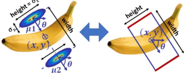
Ghazaei et al. (2018) used an encoder-decoder architecture to detect grasp points. The network mapped RGB images to belief maps that predict the position of the gripper plates. This belief map representation is used as a replacement of the rectangle representation, as seen in Figure2.5. Morrison et al. (2018) also used an encoder-decoder architecture to produce three feature maps representing a grasp pose at each pixel. The first feature map predicted the grasp quality, the second one the gripper opening and the last one the gripper angle. Similar work is presented in Wang et al. (2019).
Figure 2.5 – The belief map grasp representation, an alternative to the grasp rectangle repre-sentation. CNN auto-encoders are trained to output a probability map for the gripper’s finger positions. Figure from Ghazaei et al. (2018).
J. Cai et al. (2019) took an approach similar to the auto-encoder approaches cited before, but with a key difference. Like previous approaches, the authors predict a grasp probability at each pixel of the image. However, instead of predicting a grasp score for each discrete angle of the gripper, the authors directly rotated the input image to horizontally align the grasp with the image. To find the best grasp in a scene, they fed 16 rotated images, representing 16 discrete rotations of the gripper, and selected the grasp that had the best score among the 16
output feature maps. The authors reported a performance of 93 % on a physical benchmark consisting of grasping household objects. Importantly, this paper contains work that is very similar to some of our preliminary work that we present in Chapter 3.
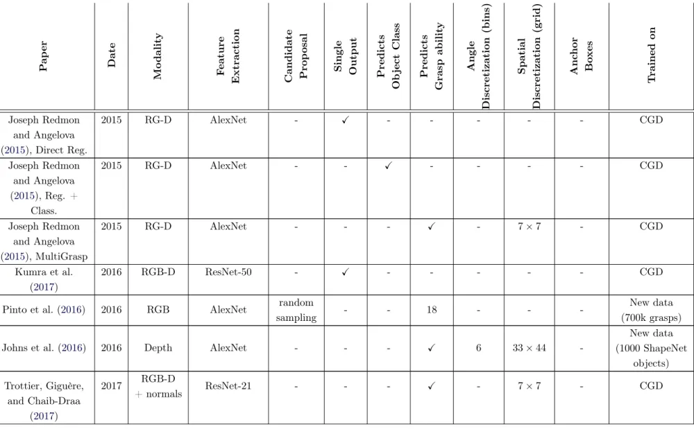
Table 2.1 – Comparison of deep learning approaches to grasping P ap er Date Mo dalit y F eature
Extraction Candidate Prop
osal Single Output Predicts Ob ject Class Predicts Grasp abilit y Angle Discretization (bins) Spatial Discretization (grid) Anc hor Bo xes T rained on Joseph Redmon and Angelova (2015), Direct Reg. 2015 RG-D AlexNet - X - - - CGD Joseph Redmon and Angelova (2015), Reg. + Class. 2015 RG-D AlexNet - - X - - - - CGD Joseph Redmon and Angelova (2015), MultiGrasp 2015 RG-D AlexNet - - - X - 7 × 7 - CGD Kumra et al. (2017) 2016 RGB-D ResNet-50 - X - - - CGD
Pinto et al. (2016) 2016 RGB AlexNet random
sampling - - 18 - -
-New data (700k grasps)
Johns et al. (2016) 2016 Depth AlexNet - - - X 6 33 × 44
-New data (1000 ShapeNet objects) Trottier, Giguère, and Chaib-Draa (2017) 2017 RGB-D + normals ResNet-21 - - - X - 7 × 7 - CGD
Mahler, J. Liang, et al. (2017)
2017 Depth Custom antipodal
sampling X - X - - - Dex-Net 2.0
Zhou et al. (2018) 2018 RGB ResNet-50/101 - - - X 6 10 × 10 6
on angle CGD
Park, Seo, et al. (2018a)
2018 RGB-D DarkNet-19 - - - X 18 Dense
(FCNN)a 7 ratiob CGD
Chu et al. (2018) 2018 RG-D ResNet-50 196 ROI - - X 19 +
no angle
-3 scalec+
3 ratio CGD
Zhang et al. (2018) 2018 RGB ResNet-101
Faster-RCNN 300 ROI - X X - - 4,6
New data (100k grasps) Park and Chun
(2018)
2018 RGB-D ResNet-32 4 ROI - - X - - - CGD
J. Cai et al. (2019) 2018 RGB Custom - - - X 16 Dense
(FCNN) -New data (6.4k grasps) L. Chen et al. (2019) 2019 RG-D Custom - - - Dense (FCNN) - CGD V. Satish et al. (2019)
2019 Depth Custom - - - X 16 Dense
(FCNN) - Dex-Net 2.0
d
a
A grasp prediction is made at each pixel of the feature map, instead of having a fixed grid-size. It enables to process images with different resolutions.
bDefault aspect ratio of the anchor boxes, being the ratio between the width and the height of the bounding box. cDefault scale of the bounding box, representing its relative size in the image.
2.3
Dynamic approaches
This section provides a brief overview of dynamic approaches to grasping. It is not meant to be exhaustive nor explain in depth the theory behind robotic arm control and planning, as our research focused on one-shot approaches. However, some work on dynamic grasping bring valuable insight that may be useful when tackling one-shot grasp detection. In this section, we thus look into the family of approaches where a deep neural network evaluates the probability of a gripper motion command to result in a positive grasp. This is usually part of a framework where, at each discrete time step, one sample and evaluate candidate gripper commands (motion or closure). Having a dynamic view of the world, work in this category often relies on a deep reinforcement learning formulation (Hester et al., 2018).
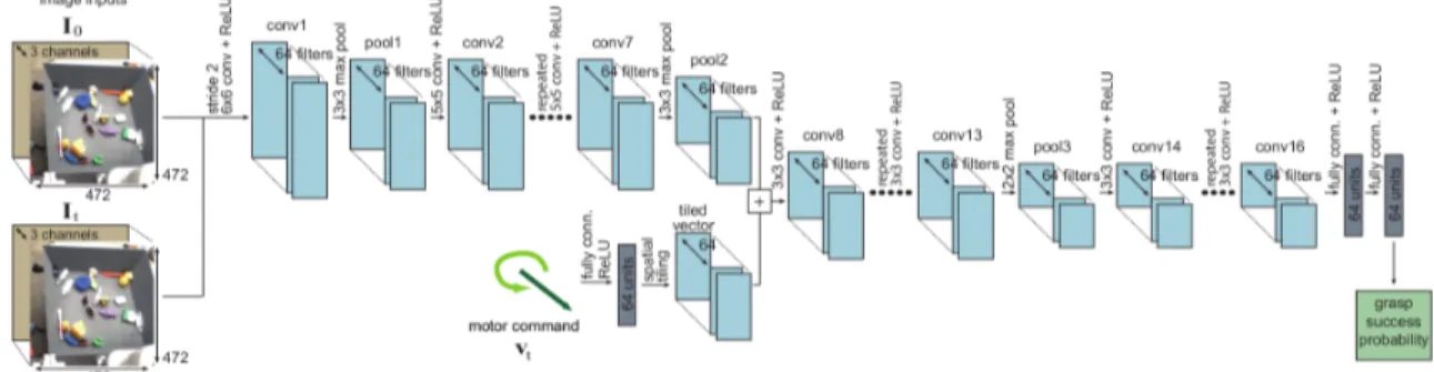
The most notable work in this category is by Levine et al. (2018), where they gathered a large-scale dataset by trial-and-error (see Section 2.4.1 for more details). Using this data, they trained a convolutional neural network to evaluate the outcome of a command, being the probability of grasping an object in a cluttered box. The network had two input images. The first one was a pre-grasp image while the second image was the current image, occluded by the robotic arm in action. The robot arm motor command vt was another input of the network.
It was integrated to the image information through late fusion, after passing through a fully-connected layer. The architecture is depicted in Figure 2.6. At evaluation time, the best command was chosen via the cross-entropy method (Rubinstein et al., 2016), a derivative-free optimization method.
Figure 2.6 – Network architecture for dynamic grasping control from Levine et al. (2018). Given a pre-grasp image, a current image including the gripper and the input command, the network outputs the probability of successfully lifting an object.
The authors showed that their method could lift a random object without replacement in a cluttered bin 90 % of the time, which is 17.5 % better than a baseline open loop method that statically detect the best grasp location.
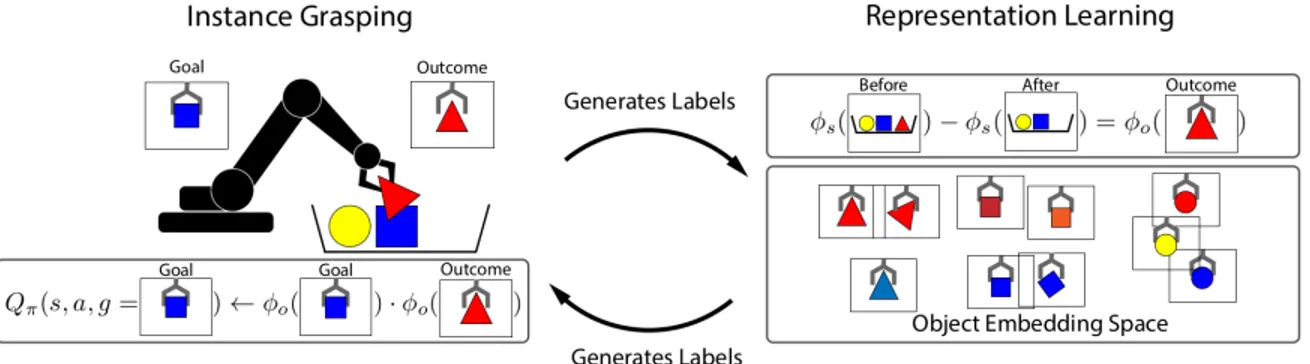
While Levine et al. (2018) learned a policy to lift any object in a cluttered bin, Jang, Devin, et al. (2018) learned a policy for instance localization and goal-directed grasping tasks on the same data, without any localization or classification annotations. To do so, they presented
Grasp2Vec, an object-centric visual embedding learned with self-supervision. The main idea is depicted in Figure 2.7, where the goal is to grasp a blue square object. However, in this example, the arm instead picked up a red triangle object via random grasping. Images of both outcomes are mapped to an embedding space, via a learned φo function. Embeddings of the scene before and after grasping the object are also computed via another learned function, φs. To learn which object was picked up without explicit labelling, the following embedding
property was enforced: the embedding of scene pre-grasp minus the embedding post-grasp must equal the embedding of the picked-up object. This is depicted in the top-right of Fig-ure 2.7. Enforcing this property created a learned embedding space where the object that were similar in color or shape were close to each other. On the bottom-left of Figure2.7, there is an illustration of how to update the policy by penalizing the cosine similarity between the embeddings of the goal object and the picked object.
Figure 2.7 – Overview of the Grasp2Vec approach (Jang, Devin, et al.,2018), an object-centric visual embedding learned with self-supervision. The network learns localization and instance retrieval without explicit labels, by enforcing consistency in embedding space.
Related work on embedding for grasping includes Sung et al. (2017). There, the authors showed how to map natural language, point clouds and grasping trajectories to a common embedding space, enabling the generation of grasps based on natural language commands. Yan et al. (2018) presented an approach that, from a single depth image, learned to reconstruct an inner 3D representation of the object to grasp. They did so without any 3D model supervision, by re-projecting the inner 3D representation to a depth image and comparing it to the actual observed depth image. The authors showed that such geometry-aware architecture led to about 10 % relative improvement from a baseline that did not reconstruct an inner 3D representation. Avi Singh et al. (2017) tackled a similar problem to Grasp2Vec. The authors used weak su-pervision to learn robot interaction. They trained an agent on a dataset consisting of two parts. The first one contained a few strong supervision examples of robot interactions in a single environment. The second part contained many weak supervision examples, consisting of annotations indicating which objects were present in the images. This part of the dataset had no interaction supervision whatsoever. They showed that using techniques from unsuper-vised domain adaptation, multitask learning and visual attention, the agent could generalize
to different environments than the one it had interaction supervision. Jang, Vijaynarasimhan, et al. (2017) developed a similar method that also used attention and weak supervision. The authors developed a two-stream system. Given a pre-grasp image, a current image and a com-mand, a ventral stream learned to classify which object will be picked up and a dorsal stream learned to predict if a grasp will result in a successful outcome. This architecture disentangled spatial and semantic inference. The authors showed that their two-stream method outper-formed baseline methods that did direct grasp detection on the task of semantic grasping. Their method grasped the correct object in a clutter more than twice as often.
2.4
Grasping Datasets
As for all machine learning applications, the robot grasping problem is ruled by a core problem: acquiring data. Nevertheless, there are challenges specific to machine learning in robotics. First, generating ground truth annotations is itself a challenging problem. A human can do manual annotations just as in an object detection task (see Section 1.2.2). However, just because a human operator thinks that a grasp annotation is positive does not mean much if it has not been verified on a real robot. Also, the human operator can introduce a bias in the training database, by favoring certain annotations over others. On the other hand, working without a human in the loop brings its own challenges. For instance, one could decide to work entirely in simulation. Nonetheless, this is susceptible to the reality gap problem (see Section 1.3 more details). One could also gather data on real hardware by trial and error. Although feasible (see Section 2.4.1), this approach is very expensive, cumbersome and time consuming. Moreover, as the gripper wears out over time, it means that the domain of the data collection and its outcome slowly drifts over time.
All those considerations explain the vast diversity in datasets that are available for robot grasping. In the rest of this section, we provide a brief overview of those that are relevant to deep learning. They are summarized as well in Table2.2.
Table 2.2 – Summary of the grasping datasets used in deep learning research Dataset Real Sensors Number of Images Modality Number
of Grasps Hand Type Labels from Dynamic
Mesh P oin t Cloud R GB Depth
Cornell (Jiang et al.,2011) Yes 1035 X X 8019 Parallel Gripper Human No
YCB (Calli, Arjun Singh, et al., 2017)
Yes 600 X X X X - - -
-KIT (Kasper et al.,2012) Yes 145 objects/
1569 meshes X X 10k Three-finger/ Human-like Rules No
Pinto et al.,2016 Yes 50k X X 50k Parallel Gripper Random No
Levine et al.,2018 Yes 800k X X 800k Parallel Gripper Random Yes
Jacquard (Depierre et al.,
2018)
No 54k X X 1.1M Parallel Gripper Random No
Dex-Net 2.0 (Mahler, J. Liang, et al.,2017)
Both 6.7M X 6.7M Parallel Gripper Rules No
G3DB (Kleinhans et al.,
2015)
No 110 X - - -
2.4.1 Real World Datasets
Cornell Grasping Dataset
The Cornell Grasping Dataset (CGD) (Jiang et al., 2011) is the most widely seen grasping dataset in the literature. It consists of 1035 images of 280 different objects, which have been manually annotated by humans. For each image, there are several positive and negative grasps. This dataset uses the grasp rectangle representation for grasp annotations (see Section 2.1). The CGD has been used extensively in grasping research (Joseph Redmon and Angelova (2015), Park and Chun (2018), Zhou et al. (2018), Trottier, Giguère, and Chaib-draa (2017), S. Caldera et al. (2018), and Park, Seo, et al. (2018b) for example). As this dataset was collected before the deep learning era, the number of examples is fairly small. This can lead to overfitting, thus bad generalization to real world conditions. Furthermore, there is a bias coming from humans selecting grasp points that “look” right. According to Pinto et al. (2016), human labelling is “biased by semantics”. For instance, if we ask a person to annotate a mug, he would have a bias toward labelling grasp points on the handle, even though there are many more valid grasp points on the object for a robotic gripper. Pinto et al. (2016) also remarked that exhaustive labelling is impossible. Finally, the objects are placed on a uniformly white background, making it visually unchallenging. All these reasons make the Cornell Grasping Dataset fall short for thorough grasping system training and evaluation.
KIT
The KIT object models database (Kasper et al.,2012) is a database of 145 objects. It contains 3D meshes and RGB images of the objects. Also, KIT contains grasp annotation for three types of hands: the three-fingered Schunk Dexterous hand, the four-fingered Schunk Anthro-pomorphic Hand (left and right hands) and the DLR/HIT Five-Finger Hand (left and right hands). Grasp annotations are only available for around 100 of the 145 objects. There are approximately 10k grasp annotations in total1. These annotations are pre-computed using a rule-based approach, as described in Xue et al. (2009).
This dataset is a predecessor of YCB (see Section2.4.1). KIT and YCB are very similar, with a few key differences:
— YCB uses consumer-grade hardware, such as Canon Rebel cameras and PrimeSense Carmine sensors. On the other hand, KIT uses commercial grade material, such as the Konica Minolta Vi-900 3D digitalizer.
— The RGB images from KIT have a much lower resolution (1394 × 1038 pixels, or around 1.4 megapixels) compared to YCB (12.2 megapixels).
— KIT contains more objects but the objects are much less diverse in shape.
1. The number of grasp annotations is not available on KIT’s website nor in the paper. The approximation is based on the estimate of 15 annotations per hand type per object.
Still, the meshes from KIT are high quality and can be used for benchmarking grasping systems.
YCB
The YCB dataset (Calli, Arjun Singh, et al., 2017) is a joint effort between Yale, CMU and Berkeley Universities to generate a high quality dataset for robotic manipulation of real-life objects. It contains 3D scans of 77 household objects such as fruits, tools, bottles, boxes and so on. Unlike KIT, the objects are easily available for purchase. For each object, the following information is available: the object’s weight, 600 high resolution RGB images, 600 RGB-D images, segmentation masks, camera calibration information, a point cloud and five sets of textured 3D meshes.
The RGB images are captured from five 12.2 megapixel Canon Rebel T3. The RGB-D images come from five PrimeSense Carmine sensors. These sensors are mounted on a BigBIRD setup that provides images from five different viewpoints. To have even more viewpoints, a target object is placed on a computer-controlled turntable. Figure 2.8 shows this data acquisition setup.
The five sets of 3D meshes come from two different sources. First, there is a 3D reconstruction of RGB and RGB-D images using two different techniques (Poisson and TSDF reconstruc-tion). Second, a Google Scanner setup gives the three other sets of meshes at three different resolutions (16k, 64k and 512k vertices).
This dataset has no manipulation annotation, meaning that it cannot be used for learning to grasp. However, it is useful for benchmarking grasping systems. Such a benchmarking protocol is described in Calli, Walsman, et al. (2015). Also, one could use such a dataset to learn pose estimation in a known object grasping framework (see Section 2.5 for grasping known object ).
Pinto’s Random Grasp Dataset
Pinto et al. (2016) presents a dataset of random grasps collected by trial-and-error on a real robot. The data collection setup consist of a Baxter robot, a parallel gripper and a Kinect V2 sensor that is set over a large table. On the table, there are multiple objects that are placed apart from each other, never overlapping.
The collection procedure goes as follow. First, a region of interest is detected using an off-the-shelf Mixture of Gaussian (MOG) background suppressor2. This steps reduces the negative grasp attempt ratio. Then, a grasp coordinate and a gripper angle are sampled from a uniform distribution in the foreground region. The robot then executes the grasp and tries to lift the