Negotiation Game for Joint IT and Energy Management in Green Datacenters

Any correspondence concerning this service should be sent

to the repository administrator:

tech-oatao@listes-diff.inp-toulouse.fr

This is an author’s version published in:

http://oatao.univ-toulouse.fr/26288

To cite this version: Thi, Minh-Thuyen and Pierson, Jean-Marc and

Da Costa, Georges and Stolf, Patricia and Nicod, Jean-Marc and

Rostirolla, Gustavo and Haddad, Marwa Negotiation Game for Joint

IT and Energy Management in Green Datacenters. (2020) Future

Generation Computer Systems, 110. 1116-1138. ISSN 0167-739X

Official URL: https://doi.org/10.1016/j.future.2019.11.018

Open Archive Toulouse Archive Ouverte

OATAO is an open access repository that collects the work of Toulouse

researchers and makes it freely available over the web where possible

Negotiation

game for joint IT and energy management in green datacenters

Minh-Thuyen

Thi

a

_,

_{Jean-Marc Pierson}

a,∗

_,

_{Georges Da Costa}

a

_,

_{Patricia Stolf}

a

_,

_{Jean-Marc Nicod}

b

_,

_Gustavo

Rostirolla

c

_,

_{Marwa Haddad}

b

a _{IRIT, University of Toulouse, CNRS, INPT, UPS, UT1, UT2J, France} b FEMTO-ST, CNRS, Univ. Bourgogne Franche-Comte, UTBM, France c LAPLACE, University of Toulouse, CNRS, INPT, UPS, France

Keywords: Datacenter Renewable energy Game theory Negotiation a b s t r a c t

As the power demand of datacenters is increasing sharply, a promising solution is to power datacenters locally by renewable energies. However, one of the main challenges when operating such green datacenters is to conciliate the intermittent power supply and the power demand. To deal with this problem, we view the green datacenter as two sub-systems, namely, Information Technology (IT) sub-system which consumes energy, and electrical sub-system which supplies energy. The objective is to find an efficient trade-off between the power demand and power supply, respecting the operational requirements of both sub-systems (i.e., the requirements on utility, or monetary gain, which includes monetary revenue and monetary cost). First, we analyze the problem by a black-box approach. In this approach, the models of the two sub-systems are unknown to each other, and the two sub-systems negotiate by exchanging their power preferences. However, we found that the black-box approach cannot guarantee stable solutions in term of execution time and generational distance (which is the distance between a solution and the Pareto front). Then we introduce a semi black-box approach, in which the two sub-systems are modeled as the buyer and the supplier in a buyer–supplier negotiation game. We propose an algorithm that allows the buyer and supplier to negotiate, seeking for an efficient trade-off between the power demand and power supply. The analytical results show that the semi black-box algorithm converges to equilibrium, and these results are then confirmed by experimental results. We conduct the experiments by implementing a middleware of a datacenter powered by renewable energies. The experimental results show that the semi black-box algorithm improves significantly the stability, quality of service (QoS) and utility of the datacenter, compared to other algorithms. In term of stability, compared to the black-box algorithm, the semi black-box algorithm reduces the standard deviation of execution time and generational distance by 23 and 27 times, respectively. In term of QoS and utility, the semi black-box algorithm outperforms the algorithms that do not consider joint IT-energy management, as well as the algorithms that do not utilize a semi black-box design.

1. Introduction

As the demand for cloud services has been growing over recent years, the energy consumption of datacenters is increasing rapidly. A number of studies have showed intensive data and reports on this increase [1–4]. The consumed electricity of data-centers worldwide can reach 8000 billion kilowatt hours (kWh) in

∗ _{Corresponding author.}

2030 if efficient control methods are not developed [3]. In the US, the datacenters consumed 100 billion kWh of electric energy in 2015, and this consumption is expected to be 150 billion kWh in 2022 [2]. On the other hand, the traditional/brown energy sources are becoming less preferable, due to economic and environmental concerns. One promising solution is to use renewable energies to locally power datacenters, avoiding both greenhouse gas emission and electricity distribution loss. We consider a green datacenter that is entirely supplied by renewable sources (namely, wind turbines (WT) and photovoltaic panels (PV)), and storage devices (namely, batteries (BT), electrolyzers (EZ) and fuel cells (FC)). However, one of the main challenges of building this datacenter is to conciliate the intermittent energy production and the con-tinuous operation of the datacenter. The production of renewable

E-mail addresses: minh-thuyen.thi@irit.fr (M.-T. Thi),

jean-marc.pierson@irit.fr (J.-M. Pierson), dacosta@irit.fr (G. Da Costa),

patricia.stolf@irit.fr (P. Stolf), jean-marc.nicod@femto-st.fr (J.-M. Nicod),

gustavo.rostirolla@laplace.univ-tlse.fr (G. Rostirolla), marwa.haddad@femto-st.fr

(M. Haddad).

energies such as WT and PV highly depends on environmental conditions, so we need to coordinate this intermittent energy production with the energy demand, in order to guarantee a high quality of service (QoS) for cloud users.

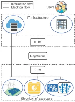
To deal with this problem, we model the datacenter with one Negotiation Module (NM) connecting to two sub-modules, namely Information Technology Decision-support Sub-module (ITDM) and Power Decision-support Sub-module (PDM). The ITDM manages the scheduling of datacenter workload, while the PDM manages the scheduling of electrical sources. The scheduling of both ITDM and PDM are considered jointly, with the support of the NM. This NM manages the negotiation between the PDM’s power supply and the ITDM’s power demand. When the power supply and power demand are mismatched, the NM aims to find a compromise between them. We provide two generic models for the ITDM scheduler and PDM scheduler; in this way, the proposed negotiation algorithms can work with any scheduler that is implemented based on these generic models.

As a straightforward approach toward a distributed design, we first propose a black-box negotiation algorithm, named Schedul-ing Based Negotiation (SAN). We define that a power profile is a set of power values associated with a time interval. In this black-box approach, each Decision-support Sub-module (DM) learns about the other DM through exchanging power profiles. These profiles, called hints, allow each DM to learn about the pre-ferred power of the other DM. Each DM is expected to gradually propose more relevant profiles based on the similarity to the hints. However, we found that the black-box approach cannot guarantee stable solutions in term of execution time and

gen-erational distance. In brief, generational distance is the distance

between a solution and the Pareto front, where Pareto front in a multi-objective problem is the boundary defined by the set of non-dominated solutions. Then, we show that a semi black-box approach is more relevant to deal with this kind of problem. We model the problem as a buyer–supplier negotiation game, and based on this game, we propose a negotiation algorithm named Game Theory Based Negotiation (GAN). In this game, the ITDM and PDM are modeled to become two game players, named IT-Player and PD-Player. These two players negotiate with each other as an energy buyer and an energy supplier. Our goal is to find an efficient compromise between the players, respecting their operational requirements. The final solution is a mutually acceptable profile for both players.

We use a buyer–supplier model because this model reflects the buying-supplying relationship between the IT sub-system and the electrical sub-system. Moreover, in a negotiation problem, when two parties negotiate on a common resource, each party should consider its willingness when compromising. This is be-cause a same amount of resource may be beneficial differently to each party. This property can be addressed by the pricing process in a buyer–supplier partnership.

We utilize a semi black-box model in order to retain the benefits of both black-box and non-black-box approach. In a semi black-box approach, the IT-Player and PD-Player are modeled independently, rather than integrally as in a centralized approach. However, unlike the black-box approach, the players can ex-change more specific information to learn about the direction to negotiate. On the other hand, our problem is a large-timescale problem, in which the decision can be made every several days. However, we found that a semi black-box approach is more beneficial than a centralized approach. Firstly, each player is not required to gather a lot of information from the other player. The independence between two players facilitates the design process and reduces the involvement in case of modifying one player. Secondly, we propose to run the negotiation algorithm regularly in a smaller timescale, e.g., every 6 h, even when there is no

request from the players. In this way, the negotiation algorithm can be run in an overlap manner, i.e., it is run every 6 h, to find a negotiation solution for 3 days. Finally, a decentralized approach facilitates the design of a multi-timescale negotiation, which is one of our future works. In this multi-timescale negotiation, we first find a long-term solution, then based on this solution, we find multiple short-term solutions, within the long-term period.

The proposed game is a sequential and alternate-move game, rather than a one-shot game. The players’ strategies (i.e., schedul-ing solutions) do not belong to a deterministic space, so it is highly complex to solve the game analytically using a one-shot non-cooperative approach. Moreover, this sequential game has perfect information, since each player knows the decision taken by the other player. However, the game is neither a complete nor incomplete information game, because even though the players know the rules of the game (e.g., pricing information), the players’ payoffs are not common knowledge.

The contributions of this research are as follows.

•

We model the problem of joint IT and energy management for datacenters entirely powered by renewable energies, then analyze that problem using a black-box and a semi black-box approach. We propose two generic models for the ITDM and PDM (section 3), then any scheduler that is implemented based on this generic model can work with the negotiation algorithms.

•

After showing the instability of the black-box approach (sec-tion 4.2), we propose a buyer–supplier negotiation game for the problem (section 5), then introduce a negotiation algorithm to solve the game (Sections 6and 7). We show that, analytically and experimentally, the proposed algo-rithm converges to equilibrium.

•

We set up a middleware to verify the proposed algorithms, and to evaluate the performance of the whole system. We show that the proposed negotiation algorithm can achieve efficient trade-offs between the utilities (i.e., monetary gains) of the IT and electrical sub-systems.

2. Related works

Recently there are a number of studies about datacenters partially or entirely powered by renewable energy. Some of them consider only energy management, some others consider only IT management, and some others jointly consider IT and energy management. Some methodologies of the energy manage-ment problem are power source coordination [5], [6], and power provisioning [7]. Some methodologies of the IT management problem are IT job scheduling [8–10], virtual machine migra-tion [11], shifting demand in time/demand response manage-ment [12,13], assigning IT jobs to computational resources, [14,

15], and Dynamic Voltage and Frequency Scaling (DVFS) [16]. There is also some literature that proposes to combine multiple methodologies, e.g., scheduling IT jobs over time, assigning IT jobs to servers/VMs, controlling the states of servers/VMs, and assigning VMs to hosts [17,18]. From the perspective of demand

response, we can also categorize those studies by temporal load

balancing (e.g., shifting demand in time), spatial load balanc-ing (e.g., assignbalanc-ing IT jobs to multiple computational resources), equipment state management (e.g., DVFS), and additional storage management.

However, there are not many studies that provide a detailed consideration of joint IT and energy management in green data-centers. Some studies that have certain levels of that considera-tion are [19–25]. Among them, the articles [19] and [20] are from a same research work; also, the articles [23,24], and [25] are from a same research work.

Some studies of Goiri et al. focus on IT scheduling with re-spect to predicted renewable sources [26], or focus on developing a research platform for green datacenters [19,20]. The authors proposed Parasol, which is a prototype of datacenter powered by solar energy, batteries, and net metering. The authors also introduced GreenSwitch, a scheduler for workload and energy sources. That research provides two main contributions: (1) the analysis of main trade-offs in the datacenters that are pow-ered by solar and/or wind energy, and (2) the design of Parasol and GreenSwitch. The authors analyze three trade-offs, namely

grid-centric approach and self-generation approach, space and cost

of solar energy, and space and cost of wind energy. In [20], the

GreenSwitch tries to minimize the cost of grid energy, with respect to the workload and the battery lifetime. The experiments of Parasol and GreenSwitch prove that an intelligent manage-ment of IT workload and energy source can reduce operation cost significantly. However, only solar panel is considered in [19] and [20]. Moreover, the IT scheduling in that research is lim-ited. At each time period, the scheduling algorithm selects which energy source (i.e., renewable, battery, and/or grid) and which storage medium (i.e., battery or grid) to use.

The research in [21,22,27] and [28] also considers joint IT and energy management, though the energy management is limited. Li et al. [22] presented two methods to maximize the utilization of renewable energy in a small/medium-sized datacenter. The first method is an opportunistic scheduling, which suggests to run more jobs when renewable energy is available. The second method is to store renewable energy surplus to use later when the renewable energy supply is low. The experiments are set up with real-world job workload and solar energy traces. The authors also show that the proposed methods can reduce the demand for energy storage. However, the proposed methods have simplified the management of power sources. This management focuses on controlling the storage devices with respect to their charac-teristics, e.g., battery depth-of-discharge, battery charging rate limit. In [21], the authors introduced a priority-based scheduling, considering the battery state and the renewable energy forecast. The scheduling uses genetic algorithm to allocate jobs, taking into account the storage capacity and the available solar energy. In general, that research focuses on virtual machine scheduling, taking into consideration the solar panel production. In [27], the authors also introduce an adaptive job scheduler with respect to the energy production forecast but of both solar and wind sources. The objective is to decrease the number of canceled or violated jobs, and increase the efficient usage of the green energy. Similar to [21], the research in [27] focuses on jobs scheduling with regard to renewable energy production. The jobs are either web services or batch jobs; and the authors assume that each server has one web services request queue, and one or more batch jobs slots. Web services are executed when there are available computing resources and there is enough brown energy to maintain these services. In [28], Leo et al. proposed a heuristic IT scheduling algorithm for datacenter powered by renewable energies and the grid. The algorithm takes into account a limited knowledge of the power sources. Specifically, each source is supposed to have a predicted function that provides the estimation of the available energy over time. Then the algorithm takes this prediction as an input in order to schedule IT jobs for the datacenter.

The project DATAZERO1 _{[23–25] is among the first studies}

that proposes the architecture of datacenters entirely powered by renewable energy, with a detailed consideration of joint IT and energy management. The works in [23] introduced the design of the architecture, while the research in [24] presented the

1 _{www.datazero.org.}

Table 1

Notations of datacenter model. Symbol Name Description

T Time window T is a constant; T is equal to the number of time steps in each profile; in experiment, T=72 (h) x Power profile Power profile has the form

x= {x1, . . . ,xi, . . . ,xT},i=1, . . . ,T, where xiis the power value at ith time step; the unit of power value is Watt (W)

u(·) Utility The utility of a DM; the utility in the black-box approach is normalized to [0, 1] and has no unit, whereas the utility in the semi black-box approach is the monetary gain, which has the unit Euro and is not normalized

r(·) Revenue The revenue of a DM; similar to the utility, the revenue in the black-box approach has no unit, whereas the revenue in the semi black-box approach has the unit Euro

c(·) Cost The cost of a DM; the cost in the black-box approach has no unit, whereas the cost in the semi black-box approach has the unit Euro J(b) Number of

batch jobs Number of batch jobs that are being processed byITDM J(s) Number of

service jobs Number of service jobs that are being processedby ITDM J Number of all

jobs

Number of service and batch jobs that are being processed by ITDM; J=J(b)+J(s)

d(x,y) Distance Distance between two profiles x and y; distance can be measured by Mean Square Error or Pearson correlation

ε Distance

threshold

Threshold used in stopping criteria of the negotiation algorithms; this threshold is set through experiment parameters

management of power demand, and the technical report [25] presented the management of power supply. In this paper, we propose the negotiation between the power demand and power supply. As a part of the project, this paper presents the results of negotiation as well as the performance of the whole system. 3. Datacenter model

3.1. Generic model

We define that a power profile (or profile) x is a set of power values, associated with a time window, denoted as x

= {

x1

, . . . ,

xT

}

, where T is the length of the time window. Depending on each

specific context, a profile may have other names, e.g., candidate

profile/candidate or hint profile/hint. Table 1 is the list of main

notations used in our datacenter model.

We design a generic model for the DMs, then any scheduler whose implementation follows this model can work with the proposed negotiation algorithms. In the generic model, the ITDM is responsible for scheduling the IT workload in data center. Sim-ilarly, the PDM is responsible for scheduling the energy sources and storage devices. The DMs run scheduling algorithms to find multiple feasible scheduling solutions, and the negotiation mod-ule helps to find a compromised solution from those scheduling solutions (Fig. 1). The proposed negotiation algorithm is a turn-based approach, i.e., when the ITDM schedules, the PDM does not, and vice versa.

The two schedulers of the two DMs are described as follows.

•

ITDM scheduler: this is an IT job scheduler; with each scheduling solution, this scheduler generates a correspond-ing power profile. Specifically, with respect to each schedul-ing solution, the scheduler computes the power profile

needed to execute the scheduled jobs (including both ser-vice and batch jobs).

•

PDM scheduler: this is a power sources scheduler; with each scheduling solution, this scheduler generates a corre-sponding power profile, which represents the power output from the electrical components (including energy sources and storage devices).

3.1.1. ITDM utility

The schedulers are able to output multiple feasible scheduling solutions. Each solution corresponds to a power profile, called

candidate. Then, the negotiation solution is selected based on the

utility of the candidates. We explain in detail this selection in the next sections. For each profile x, the ITDM’s utility u(x) is com-puted based on the Amazon pricing2 _{for on-demand instances,}

which is given as

u(x)

=

r(x)

−

c(x)

,

(1)

where the revenue r(x)

=

g(x)

−

h(x), with g(x) is job execution

time multiplied by instances cost, and h(x) is the service-level

agreement (SLA) violation compensation; the cost c(x) of the black-box and the semi black-black-box approach are given differently, which will be described in corresponding sections. The SLA violation compensations of IT batch job and service job are computed differently. First, with a set of J(b) _{batch jobs, we compute their}

average due date violation

v

(b)(x) as

v

(b)(x)

=

1 J(b) J(b)

X

i=1 t_i(f )

−

t_i(d) t_i(d)

−

t_i(s)

,

(2)

where t_i(s), t_i(d)and t_i(f )are the starting time, due date and finishing time of i-job, respectively. Note that in Eq.(2), for simplicity, we abandon x on the right-hand side expression, implicitly imply-ing that the expression is computed with respect to x. Second, for service jobs, we calculate the ratio between the amount of utilized computing resources (i.e., CPU and memory) and the amount of reference computing resources. Specifically, when a set J(s) _{of service jobs fail to receive their reference amount}

computing resource, and hence, undergo QoS degradation, we calculate the under-provisioning ratio

v

(s)cpu(x) of CPU and the

under-provisioning ratio

v

(s)mem(x) of memory as

v

(s)_cpu(x)

= v

_mem(s) (x)

=

1 J(s) J(s)

X

i=1 r_i(utiz) r_i(ref )

,

(3)

where r_i(utiz) is the computing resource utilized, and r_i(ref ) is the reference computing resource. In case of CPU,

r_i(utiz)

=

X

ξ∈Ξ

σ

i,ξfξ

,

(4) and r_i(ref )

=

X

ξ∈Ξ

σ

_i(ref )_,ξ f_ξ(ref )

,

(5)

with

σ

i,ξ is the percentage of the processing element/processing

core

ξ

that is assigned to job i, fξ is the frequency of processing

core

ξ

,

σ

_i(ref )_,ξ is the percentage of reference processing core

ξ

that

the job i requests, fξ is the reference frequency of processing core

ξ

, andΞis the set of processing cores. Similar to Eq.(2), in Eq.(3), we abandon x on the right-hand side expression for simplicity. Finally, we compute the SLA violation compensation as

h(x)

= v

(b)(x)

+

1

v

cpu(s)(x)

+ v

mem(s) (x)

, v

(s)_cpu(x)

+ v

(s)_mem(x)

6=

0

.

(6)

2 _{www.aws.amazon.com/ec2/pricing/on-demand.}

Fig. 1. Datacenter model.

Note that for comparability, the values are normalized before applying the computation.

3.1.2. PDM utility

The PDM computes its utility value, associated with each profile x, as

u(x)

=

r(x)

−

c(x

,

S)

,

(7)

where S

= {

WT

,

PV

,

BT

,

EZ

,

FC

}

is the set of utilized compo-nents; the revenue r(x) of the black-box and the semi black-box approach are given differently, which will be described in cor-responding sections; the cost c(x

,

S) is normalized to [0,1], after

being computed as c(x

,

S)

=

T

X

i=1

X

j∈S P_j,i∆t E_j(max)(c (op) j

+

c (cap) j )

,

(8) where xi

=

P

j∈SPj,i

,

i

=

1

, . . . ,

T, with Pj,i is the output power

of component j at time step i (this output power is obtained from the solution of PDM scheduling); c_j(op), c_j(cap) and E_j(max)are respectively the operational cost, the capital cost (i.e., replace-ment cost) and the maximum energy produced by the power source component j during its lifetime;∆tis the duration of one time step. Note that Pj,i can be positive or negative depending

on the status of the source j (i.e, charging or discharging). We define the operational cost c_j(op) based on the characteristics of each component. This cost is the fixed amount of maintenance cost during the entire lifetime of a component. Note that the cost to purchase hydrogen for fuel cell is not considered. In this way, we only use fuel cell when hydrogen tank is not empty.

3.1.3. Difference between two profiles

In order to quantify the difference between two profiles x and y, we define the distance between them, denoted as d(x

,

y).

Though d(x

,

y) can be implemented by any method, in the

ex-periment, we use Mean Square Error (MSE) and inverse Pearson correlation to implement this distance.

3.2. A specific implementation of DMs

Based on the above generic model, we implement one ITDM scheduler and one PDM scheduler, which were described partially in our previous works [24,25]. As in [24], the ITDM scheduler is implemented with three versions of Best Fit algorithm; these versions are different on the way that the jobs are sorted: (i) due date, closest job first; (ii) arrival time, first come first served; and (iii) job size, longest one first. Each of those algorithms takes one profile as an input, called power constraint [24]. We use the PDM’s profile with highest utility for that power constraint. However, the scheduling algorithms are not required to strictly respect the power constraint, because each PDM’s profile has a relaxation value

¯ρ

, indicating how much the ITDM is allowed to violate the power constraint. For instance, when

¯ρ =

0

.

2, the power

demand can be arbitrarily lower than the power supply, but the power demand can only exceed the power supply by 20%. In other words, denoting the power constraint as l(PD)_{, the output}

profile of the scheduling algorithm must be lower than or equal to (1

+ ¯ρ

)

×

l(PD). The ITDM has three techniques to generate multiple scheduling solutions, and therefore multiple profiles. The first technique is to vary the relaxation value. The second technique is to use different versions of Best Fit algorithm. As the third technique, the ITDM supports multiple service grades, i.e., multiple QoS levels of a job. For example, video streaming service can provide multiple encoding quality levels. We define that the degraded QoS of a batch job is associated with delay violation, whereas the degraded QoS of a service job is associated with resource under-provisioning. In this way, when a job has multiple service grades, the ITDM finds one scheduling solution for each service grade. In other words, the ITDM generates mul-tiple scheduling solutions, each solution corresponds to a service grade.

As described in [25], the PDM scheduler is based on the following integer linear program.

max T

X

i=1 P_i(prod) s

.

t

.

P_i(prod)

≤

PWT,i

+

PPV,i

+

(PFC,i

+

PBT(out),i )

η

−

(P_EZ(in)_,i

+

P_BT(in)_,i)

η,

i

=

1

, . . . ,

T

,

(1

− ¯

φ

)

×

l(IT )_i

≤

P_i(prod)

≤

(

_φ

¯

₊

₁₎

_×

_l(IT )

i

,

i

=

1

, . . . ,

T

,

state of charge equations

,

electrolyzer equations

,

fuel cell equations

,

level of hydrogen equations

,

bounds of FC, EZ

,

bounds of state of charge

,

bounds of level of hydrogen

,

(9)

where corresponding to the time step i, P_i(prod)

,

l(IT )_i , PWT,i, PPV,i,

PFC,i, and PBT(out),i , are respectively the produced power, load power,

wind turbine power, photovoltaic power, power delivered by fuel cell, and power discharged from battery; P_EZ(in)_,i and P_BT(in)_,i are the power put into electrolyzer, and the power used to recharge battery, respectively;

η

is the inverter efficiency. The resolution

of the integer linear program takes the load l(IT )_{as an input [25].}

We use the ITDM’s profile with highest utility for that input. To output multiple scheduling solutions, the PDM varies the relax-ation value

_φ

¯

_{. The meaning of relaxation in PDM is similar as in}

ITDM, except the case when the power supply is higher than the power demand. For example, when

_φ

¯

₌

₀

_.

_{2, the power supply}

Table 2

Main notations of black-box approach.

Symbol Name Description

ˇ

x The set of ITDM hints ˇx= {ˇx1, . . . , ˇxm_{, . . . ˇx}M_{}, whereˇx}m_{is an} ITDM hint

ˇ

y The set of PDM hints ˇy= {ˇy1, . . . , ˇyn_{, . . . ˇy}N_{}, whereyˇ}n_{is a} PDM hint

˙

x One variable in the binary integer program(12)

˙

x= {˙x1, . . . , ˙xM_{}indicates which ITDM} hint is selected for the matched pair, for example,x˙= {0,1,0}indicates thatxˇ2

is selected for the matched pair

˙

y One variable in the binary integer program(12)

˙

y= {˙y1, . . . , ˙yN_{}indicates which PDM} hint is selected for the matched pair, for example,y˙= {1,0,0}indicates thatˇy1 is selected for the matched pair

δ(xˇ, ˇy) Minimum distance between two setsxˇ

andˇy

This minimum distance is defined as min{d(xˇ1, ˇy1),d(xˇ1, ˇy2), . . . ,d(xˇM_{, ˇy}N_)}

φ The relaxation values of ITDM hints

φ= {φ1_{, . . . , φ}m_{, . . . , φ}M_{}, where}

φm_{∈(0,1]is the relaxation value of the} hintxˇm_{; the ITDM assigns one relaxation} value to each hint

ρ The relaxation values

of the PDM hints ρ= {ρ

1_{, . . . ρ}n_{, . . . , ρ}N_{}, where}

ρn_{∈(0,1]is the relaxation value of the} hintˇyn_{; PDM assigns one relaxation} value to each hint

cannot be arbitrarily higher than the power demand, but can only be higher by 20%.

Inside the scheduling algorithms, the distance between two profiles is implemented by MSE and inverse Pearson correlation. Denoting T as the number of time steps in each profile, the MSE distance between x

= {

x₁

, . . . ,

xT

}

and y

= {

y1

, . . . ,

yT

}

is given

as d(x

,

y)

=

1 T T

X

i=1 (xi

−

yi)2

.

(10)

Note that, similar to Euclidean distance, MSE is invariant if we change the order of power values inside the profiles. In contrast, inverse Pearson correlation can recognize that change, because it can realize the trends and evolution of power values. As a result, we implement both methods and compare their performance. When using inverse Pearson correlation, the distance between x and y is given as d(x

,

y)

=

q

P

T i=1(xi

− ¯

x)2

q

P

T i=1(yi

− ¯

y)2

P

T i=1(xi

− ¯

x)(yi

− ¯

y)

,

(11)

where x

¯

and

¯

y are the averages of the sets

{

x1

, . . . ,

xT

}

and

{

y1

, . . . ,

yT

}

, respectively.

4. Black-box approach

As a straightforward approach, we introduce and analyze a black-box negotiation algorithm, named Scheduling Negotiation Algorithm. Instead of considering the whole system by a global model, we consider the sub-systems of NM, ITDM and PDM separately. The sub-problems are solved with as little specific information as possible. The only exchanged information is power profiles.

In SAN, at the first negotiation round, each Decision-support Sub-module generates its feasible profiles, called candidates, and sends them to the NM. Each DM generates its profiles without considering the other DM. As described in Section3, each profile has an associated utility. The NM selects half of the candidates of each DM as hints, and abandons the other half. The selection

is based on the weighted sum of utilities and similarity, which is called weighted similarity. We will describe this selection in detail in the next subsection. In the next negotiation round, the NM requests a DM to generate a new half of candidates. The NM selects the DM to request based on the negotiation mode, which will be also described in the next subsection. If the ITDM is selected, the NM requests this ITDM by sending to it the PDM hint with highest utility as power constraint (i.e., l(PD)_{). Similarly,}

if the PDM is selected, the NM requests this PDM by sending to it the ITDM hint with highest utility as load (i.e., l(IT )_{). As}

mentioned in the previous section, l(PD) _{and l}(IT ) _{serve as the}

inputs of ITDM scheduler and PDM scheduler, respectively. After receiving the request, the DM reschedules to generate its new half of candidates. Then the DM sends this new half to the NM. The NM combines this new half of the DM with the hints of this DM in the previous round, in order to form a new candidate set for this DM. Again, the NM selects new hint set based on the new candidate set. The process is repeated until the NM found a pair of {1 ITDM hint, 1 PDM hint} that are matched. A pair is called matched when it consists of two profiles that have maximized summation of utilities, while the distance between these two profiles is below a given threshold

ε

. Note that, in this black-box

approach, we set the ITDM’s cost c(

·

)

=

0, and the PDM’s revenue

r(

·

)

=

1.

The proposed negotiation algorithm has two stages, namely,

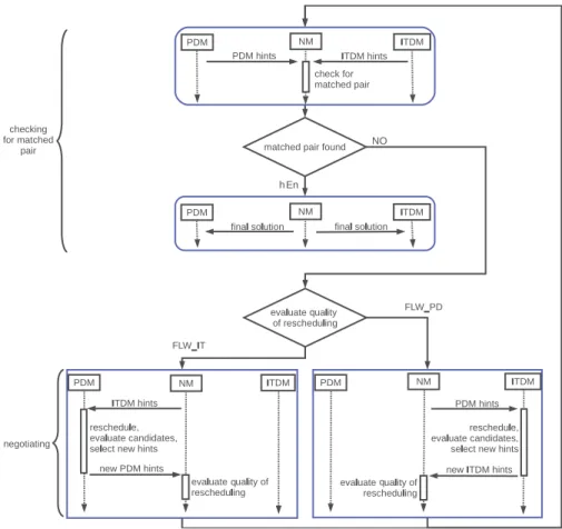
checking for matched pairand negotiating. After executing stage 1,

the algorithm checks whether to continue the stage 2 or not. We describe these two stages as follows.

•

Stage 1 - Checking for matched pair: after having a new hint set, the NM checks whether there is a pair of {1 ITDM hint, 1 PDM hint} that approximately matches with each other. If this matched pair exists, the NM returns these two hints to the DMs as the final negotiation solution. Then it is not necessary to continue the stage 2.

•

Stage 2 - Negotiating: if the NM cannot find any matched pair, stage 2 is executed. We propose a turn-based mecha-nism in which the two DMs do not reschedule at the same time. In each negotiation round, the NM determines the

negotiation mode, which indicates which DM is allowed to

reschedule at the next negotiation round. To do this, the NM monitors the quality of the rescheduling, in order to decide which DM should reschedule at the next round. In the next subsection, we describe this negotiation algorithm in detail.

4.1. Details of algorithm

InFig. 2, we show diagram of the proposed algorithm; stage 1 is depicted at the upper part, and stage 2 is depicted at the lower part of the figure. In stage 1, if a matched pair is found, the final solutions are sent to the DMs, and the negotiation stops. If a matched pair is not found, stage 2 is performed. In stage 2, the algorithm is in one of these two negotiation modes: (i) following ITDM (named FLW_IT), and (ii) following PDM (named FLW_PD). In the FLW_IT mode, the NM requests the PDM to reschedule; then the PDM reschedules to generate a new half of candidates, and sends back to the NM. Similarly, in the FLW_PD mode, the NM requests the ITDM to reschedule, then the ITDM reschedules to generate a new half of candidates. In brief, a negotiation round includes three tasks: (i) scheduling, (ii) evaluating the candidates using weighted similarity, and (iii) selecting new hints. In the FLW_IT mode, after receiving new half of candidates from the PDM, the NM evaluates the quality of rescheduling in order to decide the mode for the next negotiation round. The procedures in the FLW_PD mode follow the same processes.

The details of the two stages are provided in the following subsections.

4.1.1. Stage 1 - Checking for matched pair

We denote the set of ITDM hints asx

ˇ

= {ˇ

x1

, . . . ˇ

xm

_{, . . . , ˇ}

_xM

_}

_,

and the set of PDM hints asy

ˇ

= {ˇ

y1

, . . . , ˇ

yn

_{, . . . ˇ}

_yN

_}

_{, where M and}

Nare respectively the number of ITDM hints and PDM hints. We

describe the main notations of the black-box approach inTable 2. Stage 1 checks whether there is a pair of {1 hintx

ˇ

m_{, 1 hinty}

_ˇ

n_}

that matches. In order to find that pair, we solve a binary integer program with two variablesx

˙

andy

˙

. These variables are two

bi-nary vectors:x

˙

= {˙

x1

, . . . , ˙

xm

, . . . , ˙

xM

}

,y

˙

= {˙

y1

, . . . , ˙

yn

, . . . , ˙

yN

}

, wherex

˙

m

_{∈ {}

₀

_,

₁

_},

_m

₌

₁

_{, . . . ,}

_{M, and}

_˙

_yn

_{∈ {}

₀

_,

₁

_},

_n

₌

₁

_{, . . . ,}

_N.

Eachx

˙

m_{is a binary value, indicating thatx}

_ˇ

m_{is selected or not.}

Stage 1 is represented by the following binary integer pro-gram. max ˙ x,˙y M

X

m=1 u(x

ˇ

m_)x

_˙

m

₊

N

X

n=1 u(y

ˇ

n_)y

_˙

n

_,

s.t. M

X

m=1 N

X

n=1 (1

− φ

m)(1

− ρ

n)x

˙

my

˙

nd(x

ˇ

m

, ˇ

yn)

< ε,

M

X

m=1

˙

xm

=

1

,

N

X

n=1

˙

yn

=

1

,

˙

xm

, ˙

yn

∈ {

0

,

1

},

(12) where

•

u(x

ˇ

m_{) and u(y}

_ˇ

n_{) are the utilities of the hints x}

_ˇ

m _{and y}

_ˇ

n_,

respectively,

•

d(x

ˇ

m

_{, ˇ}

_yn_{) is the distance betweenx}

_ˇ

m_andy

_ˇ

n_,

• φ

m_and

_ρ

n_{are the relaxation values of the hints}

_ˇ

_xm_andy

_ˇ

n_,

respectively,

• ε

is the distance threshold, which is set through experiment parameters.

The binary integer program finds a pair of profiles that maximizes the summation of utilities, while the distance between these two profiles is lower than the distance threshold

ε

.

4.1.2. Stage 2 - Negotiating

In this stage, the NM continues to use the hints of the previous stage. This stage includes the scheduling process of the DMs and the evaluating process of the NM. The scheduling process is for generating multiple feasible scheduling solutions, corresponding to multiple candidates. The evaluating process is for assessing the candidates against the hints, based on weighted similarity.

We describe the FLW_PD mode as follows. Note that the FLW_IT mode undergoes similar processes. After receiving the re-quest with l(PD)_{from the NM, the ITDM reschedules to find a new}

half of candidates. Then the ITDM sends these new candidates to the NM. The NM combines the ITDM hints of previous round with the newly received candidates to form the new ITDM candidate set. Then, the NM computes the quality

w

of each ITDM candidate

xbased on weighted similarity, as follows.

w

=

N

X

n=1 u(x)

+

u(y

ˇ

n₎ d(x

, ˇ

yn₎

,

(13) where

•

d(x

, ˇ

yn_{) is the distance between the candidate x and the hint}

ˇ

yn_,

•

u(x) is the utility of the candidate x, and u(

ˇ

yn_{) is the utility}

of the hinty

ˇ

n_.

The NM selects half of ITDM candidates to become the ITDM’s new hints. Then the NM decides whether to continue the FLW_PD

Fig. 2. Scheduling-based negotiation algorithm. How to evaluate quality of rescheduling is explained in Section4.1.2.

mode or switch to the FLW_IT mode. To this end, the NM eval-uates the quality of the ITDM’s reschedule by comparing two distances: (i) the minimum distance

δ

(

·

) between the PDM hints and the ITDM hints of previous negotiation round, and (ii) the minimum distance

δ

(

·

) between the PDM hints and the ITDM’s new hints of current negotiation round. If the former is greater than the latter, we say that the quality of the ITDM’s reschedule is satisfactory. Then the NM allows the ITDM to execute another reschedule at the next negotiation round. If the former is smaller than the latter, the PDM is allowed to reschedule. The intuition behind this comparison is that, when the former is greater than the latter, we expect that the ITDM will generate new candidates that get closer to the PDM hints. To compute the minimum distance

δ

(

·

) between two sets, we compute the distance of every pair between two sets, then select the smallest distance.

The negotiation process repeats until the NM finds a pair of matched profiles, or the number of negotiation rounds reaches a given threshold. This threshold is set via an experiment parame-ter. When the NM cannot find a matched pair, the pair with the smallest distance is selected as the final solution. Then the PDM’s profile in that pair is implemented as the power supply, and there is a possibility that the performance of the datacenter is degraded when the power supply is lower than the power demand.

4.2. Stability of black-box approach

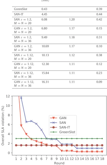
We implement a middleware of datacenter powered by newable energies in order to carry out experiments for our re-search, as described in [29]. With SAN, we evaluate and analyze the execution time, as well as the generational distance of each individual execution, as showed in Figs. 3 and 5. Generational

distanceis first introduced by Van Veldhuizen and Lamont [30],

for estimating the average Euclidean distance between a solution

and the nearest point on Pareto front. We measure this distance in order to evaluate the trade-off of our final solution. To this, we trace the generated solutions and approximate their Pareto front by finding the set of non-dominated solutions; then we measure the generational distance of our final solution to this Pareto front (Fig. 4). We note that the Pareto front is the best known approximation, because in order to compute the complete Pareto front, we need to have the set of all feasible solutions, which is highly complex to generate.

InFig. 3, we depict the execution time, grouped by the num-ber of hints. Each gray dot represents the execution time of an individual execution. The vertical line and the middle bar, respectively, represent the standard deviation and the mean, which are computed from the values of gray dots. We can see that, when the number of hints is 4, the execution time varies widely. When the number of hints is high, the execution time becomes more consistent but also grows higher. In Figs. 5and

6, we show the generational distance with respect to the number of negotiation rounds and the number of hints, respectively. In these experiments, we set the distance threshold

ε

=

1

.

12.Fig. 6

shows that the black-box model cannot guarantee stable results, in term of generational distance.

The experiments show that SAN is not able to provide highly consistent and stable results. In the next section, we propose a semi black-box approach for negotiation.

5. Semi black-box approach

To deal with the instability of the black-box approach, in this section, we propose a semi black-box approach, which includes a game model and a negotiation algorithm, named Game Theory Based Negotiation. The game has two players, namely IT-Player

Fig. 3. Execution time with respect to the number of hints.

Fig. 4. Illustration of solutions (gray dots), final solution (red square), and Pareto front (blue stars).

Fig. 5. Generational distance with respect to the number of negotiation rounds.

and Player, corresponding to the two sub-systems. The PD-Player controls the electrical sub-system, playing the role of a supplier; the IT-Player controls the IT sub-system, playing the role of a buyer (Fig. 7). The IT-Player and PD-Player have the functionality of game players, and they only use ITDM and PDM as their schedulers. With this game design, we abandon the role of the NM.

Fig. 6. Generational distance with respect to the number of hints.

Fig. 7. Game model.

We introduce the new terms order, aspiration order, aspiration

supply, and price. Among them, order, aspiration order, and

aspira-tion supplyare profiles. We will provide the detailed definitions

of aspiration supply and aspiration order in the next section. The definitions of order and price are as follows.

•

Order: a power profile, which indicates how much power

the IT-Player plans to buy from the PD-Player.

•

Price: similar to opening price in [31], price is the per-unit

payment that the IT-Player has to pay to the PD-Player, price is in Euros/kWh.

The roles of the IT-Player and PD-Player are different, specifi-cally, the PD-Player first proposes price, then the IT-Player places

order based on that price. In other words, the PD-Player controls

the price, while the IT-Player controls the order. In this way, the PD-Player is able to reflect the availability of energy in the price. In the proposed game, each player has its own objective and constraints, which are described as follows.

•

IT-Player: maximizes its utility (i.e., monetary gain), while satisfying the users’ demand. Unlike SAN where the utility is an abstract value and normalized to [0, 1], the utility in GAN is the amount of money a DM earns. Specifically, the

IT-Player utility is defined as the difference between: (i) the payment that the users give to the IT-Player, and (ii) the payment that the IT-Player gives to the PD-Player. The first payment is r(x), corresponding to an ITDM profile x, computed based on the Amazon pricing. Each ITDM profile indicates how much power the IT-Player will buy from the PD-Player. This power provides a certain computing capacity to the users; then, the users pay to the IT-Player.

•

PD-Player: maximizes its utility (i.e., monetary gain), while considering the environmental conditions and operating cost (i.e., operational and capital cost, as in Section3). That utility is defined as the difference between: (i) the payment from the IT-Player and (ii) the operating cost of the electrical infrastructure.

We depict the two players and their relationship as inFig. 7. The decision variables of the PD-Player are price and energy

source scheduling, whereas those of the IT-Player are order and job

scheduling. The players obtain scheduling solutions from the ITDM

and PDM. The PD-Player obtains the energy source scheduling solution from the PDM; similarly, the IT-Player obtains the IT job scheduling solution from the ITDM. We described the DMs’ scheduling algorithms in Section3.

The proposed game is not completely a cooperative game or a non-cooperative game. The players are partially selfish, i.e., each player maximizes its own utility, however, at some points, the players sacrifice their utility, in order to reach a negotiation agreement. We will define this sacrifice mechanism in subsec-tion6.2.

6. Overview of GAN algorithm

6.1. Terms definitions

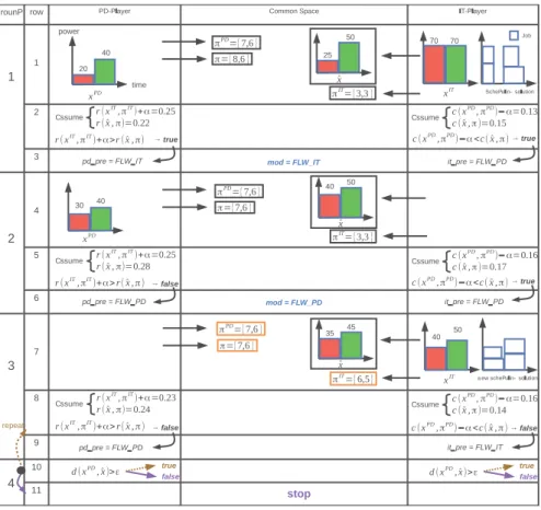
Fig. 8 shows the variables and procedures of the proposed algorithm. In the figure, we introduce some new terms.

•

Aspiration order: the power profile that the IT-Player

de-sires to order, after considering users’ demand. We also use aspiration order as the load l(IT )_{for the PDM’s scheduler.}

•

Aspiration supply: the power profile that the PD-Player

de-sires to supply, after considering the environmental condi-tions and operating cost. The final solution of the negotiation is the aspiration supply in the last negotiation round. We also use aspiration supply as the power constraint l(PD) _for

the ITDM’s scheduler.

The aspiration order and aspiration supply are used as two reference points [31]. Also, we introduce two other reference points, namely, IT incentive price and PD incentive price. In a buyer–supplier game, reference points are important; and the players can revise these points during the negotiation, in order to reach an agreement. That revision is necessary because there is a possibility that the game has negative bargaining zone [31].

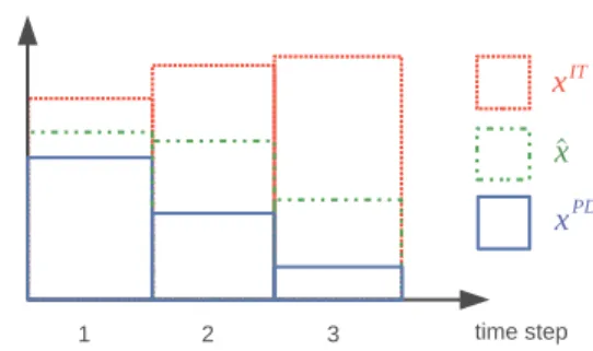
Fig. 9is an example of the aspiration supply, order, and as-piration order. In that example, the power supply of PD-Player is generally lower than the power demand of IT-Player. We suppose that the reasons are the environmental conditions, operating cost, and/or users’ demand. The PD-Player proposes the price

π

that is

inversely proportional to xPD_{. Then, the IT-Player places the order}

ˆ

x, considering the IT-Player utility and the price

π

. Since

π

is inversely proportional to xPD_{, we can expect thatx}

_ˆ

_{has similar}

curve with xPD_{. Fig. 10 shows how to generate the aspiration}

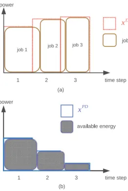
order xIT _{and the aspiration supply x}PD_{. The IT-Player generates}

xIT _{based on the scheduling solution of job 1, job 2 and job 3.}

The difference between xIT _andx

_ˆ

_{is that x}IT _{is the direct result}

of a scheduling solution, whereas

ˆ

x is the output of another

Fig. 8. Variables and procedures in the algorithm.

Fig. 9. An example of power profiles.

computation after we already had a scheduling solution. Similar to IT-Player, the PD-Player generates xPD_{based on the scheduling}

solution of available energy. We will describe in detail these gen-erations in the formulations of IT-Player and PD-Player.Table 3

summarizes the main notations in semi black-box approach. In GAN, the two modes FLW_IT and FLW_PD correspond to

follow IT-Player and follow PD-Player. Due to our turn-based

de-sign, at a time, the algorithm follows only IT-Player or PD-Player. The decision of which mode to follow is not made by any player, but by the global variable mod, as will be explained in Section7. On the other hand, the players are selfish, and they negotiate just because they foresee their benefit. Specifically, the IT-Player wants the PD-Player to follow it, i.e., the IT-Player wants the PD-Player to reschedule, in order to propose a more attractive supply. Similarly, the PD-Player wants the IT-Player to reschedule and propose a more attractive order. In this way, a problem of

selfishness may occur: both players do not want to follow each

Fig. 10. The generating of (a) xIT_{and (b) x}PD_. Table 3

Main notations of semi black-box approach. Symbol Name Description

π Price Price is in Euros/kWh, proposed by the PD-Player, indicating the per-unit payment that the IT-Player has to pay to the PD-Player, having the formπ= {π1, . . . , πT}

ˆ

x Order An order is a power profile, proposed by the IT-Player, indicating how much power the IT-Player wants to buy from the PD-Player, having the formˆx= {ˆx1, . . . , ˆxT}

πIT _{IT incentive} price

πIT _{is the price that the IT-Player can offer to} the PD-Player, i.e., willing-to-pay price;πIT _has the vector form likeπ

πPD _{PD incentive} price

πPD_{is the price that PD-Player can offer to} IT-Player;πPD_{has the vector form likeπ} xIT _Aspiration

order

xIT _{is the profile that the IT-Player desires,} with respect to users’ demand; xIT _{has the} vector form likexˆ

xPD _Aspiration supply

xPD_{indicates the power that the PD-Player} wants to supply to the IT-Player, with respect to the states of electrical components; xPD_has the vector form likeˆx

α Sacrifice

variable

This variable is used in sacrifice mechanism, making the DMs sacrifice their utility in order to continue negotiation

γ Sacrifice

step-size

γ indicates how muchαis increased every time we use sacrifice mechanism; this step-size is set though experiment parameters

To deal with this problem, we introduce the mechanism of

incen-tive pricing. In this mechanism, each player proposes an incentive

pricethat is possibly attractive to the other player. However, the

players cannot freely propose this price; they must guarantee that their utilities are not reduced if this price is used. The intuition behind this mechanism is as follows.

•

IT incentive pricing: if the PD-Player is attracted by the IT

incentive price, and the PD-Player wants this price to be

used, then the PD-Player must supply a power profile that is equal to the aspiration order.

•

PD incentive pricing: if the IT-Player is attracted to the PD

incentive price, and the IT-Player wants this price to be used, then the IT-Player must place an order that is equal to the aspiration supply.

The incentive prices are the signals of the willingness to co-operate. Incentives can be a powerful tool for the buyer to seek for agreement with the supplier [32]. In our model, we allow both supplier and buyer to use this tool. We utilize cooperative

incentive, instead of competitive incentive [32], since cooperative

incentives enable players to share cost [33] and/or revenue [34].

6.2. Sacrifice mechanism

We found that, even with incentive pricing mechanism, the problem of selfishness may still occur, i.e., both players stop negotiating while an agreement is not reached. The problem of selfishness occurs when the incentive is not attractive enough for both players to follow each other. From the system-wide perspective, this situation is unacceptable, since the system will stop working. To deal with this problem, we introduce sacrifice

mechanism. At first, both players negotiate without sacrificing. If

the problem of selfishness occurs, the players sacrifice their utility to continue negotiating, trying to reach an agreement.

A player sacrifices by giving more attractiveness to the in-centive price, even though the utility of that player is reduced. The intuition behind this is that, if the players stop negotiating without reaching any agreement, we can assume that the players and the end-users receive a very low utility (e.g., negative infinity utility); therefore, the players need to continue negotiating, even though their utility decreases. We introduce the sacrifice variable

α

, which indicates how much utility the players sacrifice. Every

time the problem of selfishness occurs, we increase

α

, raising the sacrifice quantity that each player should abide by.

6.3. Two modes of negotiation

Fig. 11depicts two sequential diagrams of two modes FLW_IT (i.e., following IT-Player) and FLW_PD (i.e., following PD-Player). Those modes are described as follows.

•

FLW_IT: The PD-Player reschedules and computes new aspi-ration supply, new price, new PD incentive price, and new mode. After that, the PD-Player sends these new information to the IT-Player. The IT-Player computes new order and new mode, then sends to the PD-Player.

•

FLW_PD: The IT-Player reschedules and computes new as-piration order, new order, new IT incentive price, and new mode. Then the IT-Player sends these new information to the PD-Player. The PD-Player computes new mode, then sends to the IT-Player.

We note that, as showed inFig. 11, if some information is not modified, it can be stored and reused. For example, in the FLW_IT mode, the PD-Player can reuse the aspiration order and the IT incentive price.

6.4. Mode controlling

In order to control the mode, we use 3 variables: IT-Player local variable it_pre

∈ {

FLW_IT

,

FLW_PD

}

, PD-Player local vari-able pd_pre

∈ {

FLW_IT

,

FLW_PD

}

, and global variable mod

∈

{

FLW_IT

,

FLW_PD

}

. Both players always run the same mode, called system mode; this mode depends only on mod. And mod,

Fig. 11. Two modes of GAN algorithm. Table 4

The determining of system mode; (*) means either FLW_IT or FLW_PD.

if then

Checking current values Updating new value Updating system mode

Variable it_pre Variable pd_pre Variable mod Variable mod System mode

FLW_IT FLW_IT (*) FLW_IT Follow IT-Player

FLW_PD FLW_PD (*) FLW_PD Follow PD-Player

FLW_PD FLW_IT FLW_IT_{FLW_PD} FLW_IT (keep unchanged)_{FLW_PD (keep unchanged)} Follow IT-Player_{Follow PD-Player}

FLW_IT FLW_PD (*) modcannot be determined System mode cannot be determined, the problem of selfishness occurs; we have to use sacrifice mechanism to solve this problem

Algorithm 1Procedures of IT-Player procedurefollow_it()

ˆ

x

←

it_place_order()

Send a message of {x

ˆ

,

it_pre

,

mod}, and wake up the

PD-Player Loop procedurefollow_pd() xIT

←

it_sched()

ˆ

x

←

it_place_order()

π

IT

←

it_est_price()

Send a message of {xIT

_{, ˆ}

_x

_{, π}

IT

_,

_{it_pre}

_,

_{mod}, and wake up the}

PD-Player Loop

Algorithm 2Mode Updating

1: procedureupdate_mode(i_pre

,

p_pre

,

g_mod)

2: if i_pre = FLW_IT and p_pre = FLW_IT then

3: return FLW_IT

4: else

5: if i_pre = FLW_PD and p_pre = FLW_PD then

6: return FLW_PD

7: else

8: return g_mod

in turn, is jointly controlled by two local variables. The two local variables cannot directly control the system mode, but instead, indirectly through the global variable. The local variable it_pre indicates the mode that the IT-Player prefers; similarly, the local variable pd_pre indicates the mode that the PD-Player prefers. Based on the current values of the variables, we update the new

Algorithm 3IT-Player Loop

1:

α

←

0,

τ

←

1

2: while d(xPD

_{, ˆ}

_x)

_{> ε}

_and

_τ

_≤

_{ITER do}

3: if it_pre

=

FLW_IT then

4: if pd_pre = FLW_PD then 5:

α

← α + γ

6: else 7: follow_it() 8: else 9: if pd_pre = FLW_PD then 10: follow_pd() 11: else

12: if mod= FLW_IT then

13: follow_it() 14: else 15: follow_pd() 16: if c(xPD

_{, π}

PD₎

_{− α <}

_c(

_ˆ

_x

_{, π}

_{) and d(x}PD

_{, ˆ}

_x)

_{> ε}

_then 17: it_pre

←

FLW_PD 18: else 19: it_pre

←

FLW_IT

20: mod

←

update_mode(it_pre, pd_pre, mod)

21:

τ

+ +

22: Sleep until received new message from PD-Player

value of mod and the system mode. Specifically, if it_pre

=

FLW_IT and pd_pre

=

FLW_IT , we will set mod

=

FLW_IT regardless of current value of mod. Similarly, if it_pre

=

FLW_PD

of the current values of mod. If it_pre

=

FLW_PD and pd_pre

=

FLW_IT , we keep the mod unchanged. If it_pre

=

FLW_IT and

pd_pre

=

FLW_PD, we cannot determine either mod or system mode. This means that we encounter the problem of selfishness, and negotiation cannot be continued. We have to use sacrifice mechanism to deal with this problem. We summarize how to determine system mode inTable 4.

If the players are completely selfish, then each player always wants the other player to follow itself, regardless of whether it foresees benefit from following the other player or not. In this way, there is high possibility that we encounter the situation when it_pre

=

FLW_IT and pd_pre

=

FLW_PD, meaning that the negotiation cannot be continued. In order to reduce the possibility of this situation, instead of designing the players to be completely selfish, we design them to be partially selfish, i.e.,

•

when the IT-Player foresees benefit from following the PD-Player, the IT-Player sets it_pre

=

FLW_PD

•

when the PD-Player foresees benefit from following the IT-Player, the PD-Player sets pd_pre

=

FLW_IT .

In this way, the problem of selfishness only occurs when both players cannot foresee any benefit of following each other. 7. Details of GAN algorithm

Corresponding to two modes, the algorithm of each player has two procedures, namely follow_it() and follow_pd(). Moreover, each player has a main loop, named IT-Player Loop (algorithm

3) and PD-Player Loop (algorithm5). Note that, in the loops, the parameter ITER is the maximum number of iterations. The two loops have the same values of ITER, distance threshold

ε

, and

sacrifice step-size

γ

; other variables and parameters are different;

especially, each player has its own value of

α

. The parameters

ITER,

ε

, and

γ

are constants, and they are set via experiment

parameters. We note that, two players have the procedures with same names, but their implementations are different. Two pro-cedures of IT-Player are showed in algorithm1; two procedures of PD-Player are showed in algorithm4. When the negotiation starts, the two main loops run in parallel. Within a loop, depend on the system mode, a procedure can be called accordingly. A player, after finishing a procedure, sends a message containing updated information to the other player. On the other hand, a loop goes to sleep after reaching its end, and wakes up after re-ceiving a new message from the other player’s procedure (i.e., line 22 in algorithm3and algorithm5).

In the proposed game, the players have the choice to stop negotiating. However, both players have the opportunity to in-crease their utility if they continue to negotiate. We define that if both players stop negotiating before reaching an agreement, each player receives a very low utility. That is why we introduce the incentive pricing mechanism and the system mode controlling. In this way, no player is allowed to unilaterally stop the negotiation process.

7.1. IT-Player algorithm

7.1.1. Overview of IT-player algorithm

Two IT-Player procedures follow_it() and follow_pd() are showed in algorithm1. During one iteration, the IT-Player Loop can call one procedure; after finishing the iteration, the IT-Player Loop sleeps and waits for new message from PD-Player. Mean-while, the called procedure starts to run; when this procedure finishes, this procedure wakes up the PD-Player Loop (algorithm

5). The two procedures are described as follows.

Table 5

Behaviors of the IT-Player Loop, depending on the updated value of mod.

if then

Updated value mod Updating behavior

FLW_IT Call follow_it()

FLW_PD Call follow_pd()

modcannot be determined; the problem of selfishness occurs

Increaseα; use sacrifice mechanism to solve the problem of selfishness

•

follow_it(): the IT-Player runs this procedure when mod

=

FLW_IT . In this procedure, the IT-Player only needs to

com-pute and sends to PD-Player the new order x

ˆ

and new modes (Fig. 11). This computation uses the price proposed by the PD-Player. The IT-Player computes

ˆ

xby the procedure it_place_order().

•

follow_pd(): the IT-Player runs this procedure when mod

=

FLW_PD. In this procedure, the IT-Player must reschedule

to compute the new aspiration order xIT_{, the new order}

ˆ

x, and the new IT incentive price

π

IT _{(Fig. 11). The}

IT-Player computes xIT_,x

_ˆ

_{, and}

_π

IT _{by the procedure it_sched(),}

it_place_order()and it_est_price(), respectively.

7.1.2. IT-Player loop

The main loop of IT-Player is showed in algorithm 3. We terminate the loop when: (i) the distance between xPD _andx

_ˆ

_is

equal or less than a threshold

ε

, or (ii) the maximum number of iterations is reached, i.e.

τ

≥

ITER. We verify these stopping

criteria at line 2 of the algorithm 3. The criterion (i) means that the power demand is approximately equal to the power supply. When the criterion (ii) is satisfied, we stop the negotiation without obtaining a compromise solution. In this case, the power supply from the PD-Player is xPD_{, and there is a possibility that the}

performance of the datacenter is degraded if the power supply is lower than the power demand.

In the loop, the IT-Player first checks and updates the sacrifice variable

α

. This check and update are done from line 3 to line 5. We need to increase

α

when both IT-Player and PD-Player stop

following each other. Specifically,

α

is increased when the loop

is not terminated but it_pre

=

FLW_IT and pd_pre

=

FLW_PD, meaning that IT-Player wants to follow itself and PD-Player also wants to follow itself. We increase

α

in order to help the players have more incentive to follow each other. We use

α

in the

condition at line 16. In that condition, c(

·

) is the cost function, indicating the IT-Player payment to the PD-Player. This condition means that, if the PD incentive price and the aspiration supply are used, the IT-Player pays lower cost than when the current price and order are used. With larger

α

, this condition is more likely to

hold, then it_pre is more likely to be set to FLW_PD (line 17). In the loop, the IT-Player calls the procedure follow_it() or

follow_pd() based on the system mode; and the system mode

depends on the values of mod, it_pre and pd_pre (from line 7 to line 15). We summarize the behaviors of the loop, depending on the modes, as inTable 5.

At the end of the loop (line 20), the IT-Player updates the global variable mod using algorithm2. This variable only switches its value when both local variables it_pre and pd_pre have switched to the same value. In this way, a player cannot unilat-erally change the system mode, which results in conflicting.

The sacrifice mechanism supports the convergence of the al-gorithm. When the players stop following each other but the algorithm still has not converged, the players are required to sac-rifice their utility by

α

, then the negotiation has more possibility

to continue. Every time the players stop following each other, we increase

α

by an amount of the sacrifice step-size, which is denoted as

γ

(line 5). The sacrifice mechanism is applied until