OATAO is an open access repository that collects the work of Toulouse
researchers and makes it freely available over the web where possible
Any correspondence concerning this service should be sent
to the repository administrator:
[email protected]
This is an author’s version published in: http://oatao.univ-toulouse.fr/21181
To cite this version:
Le Maitre Gonzalez, Esteban
and Desforges, Xavier
and
Archimède, Bernard
Assessment method of the multicomponent
systems future ability to achieve productive tasks from local
prognoses. (2018) Reliability Engineering and System Safety, 180.
403-415. ISSN 0951-8320
Assessment method of the multicomponent systems future ability to achieve
productive tasks from local prognoses
Esteban Le Maitre González
a,b, Xavier Desforges
b,⁎, Bernard Archimède
baInstituto Tecnológico de Costa Rica, Cartago, Costa Rica
bLaboratoire Génie de Production Université de Toulouse, INP-ENIT, Tarbes 65016, France
Keywords: Reliability Uncertainty
Dempster Shafer Theory Bayesian networks Prognostics Decision support
A B S T R A C T
Conditioned-based maintenance and prognostics and health management enable to optimize maintenance by scheduling the necessary repairs and replacements of technical system components according to their present and future health states. The assessment of future health states is the prognostics and health management keystone. Many technical production systems are made of numerous components implementing their functions. A method to assess the ability of multicomponent systems to carry out future production tasks is proposed to provide decision supports for production and maintenance planning for a better compromise between their objectives. It is based on components prognoses. To handle inherent uncertainties of these prognoses, the method is based on the Dempster Shafer theory and Bayesian networks inferences. Local prognoses are cate-gorized and transformed to be compliant to Dempster Shafer theory. Patterns of systems are identified for which inferences are defined. The patterns are then used to model systems and to assess their abilities to achieve future tasks. An identification of components that should first undergo maintenance is proposed. An example im-plementing a fictitious complex systems is presented to show how the provided decision supports can be used for production and maintenance planning purposes.
1. Introduction
Facing to always more competitive markets, companies invest in or develop complex technical resources for production of goods or services to improve their flexibility and their responsiveness. Therefore, the production resources become more costly. In such a context, the costly technical resources must comply the highest standards of dependability not only to satisfy return over invest criteria but also to reduce the risk of accidents causing damages to goods, people and environment. Reliability studies of such technical resources or systems are of course a major issue as well as maintaining them in operational condition with the highest level of availability for the lowest cost.
Nevertheless, the complexity of systems is always increasing. Indeed, to be more flexible and responsive, the technical systems im-plement more functionalities many components bring into operation. Because of the variety of functions, components and their technologies, the number of failures that must be considered is increasing too. The reliability assessment of multicomponent systems is to be considered not only at exploitation stage but also at design stage.
During the exploitation stage, high standards of availability and dependability of the technical production systems can be reached
thanks to the implementation of Condition-Based Maintenance (CBM) and, more recently, of Prognostics and Health Management (PHM) re-commendations while reducing maintenance costs[1–3]. CBM consists in scheduling the necessary repairs and maintenance of technical pro-duction resources from the assessment of their current conditions be-fore their failures. If PHM also consists in scheduling maintenance ac-tion before the failure of the systems, it aims at assessing the future conditions (future health) of the systems often leading to the assess-ments of their durations of use before their failures. This estimated time to failure is commonly called Remaining Useful Life (RUL)[4,5].
To make the prognoses of technical systems possible, it is necessary to predict failures of their components. In the domain of PHM, many works deal with techniques for component prognosis. They contribute to assess RULs of components, to improve the RUL assessment accuracy or to predict how degradations will evolve with time[6–10]. For this purpose, three approaches can be considered: experience-based prog-nostics, model-based prognostics and data-driven prognostics [11]. Those studies consider different kinds of components such as ball-bearings[4,12], gear trains[10,13], braking systems[14], batteries [7,8,15], gas turbines [16], etc., but also structural parts to predict crack growth[17,18]. Some studies aim at more generic approaches
Corresponding author.
However, the distributions of RULs or of the degradations after given periods of use are not always identified but works dealing with prognostics of components often provide identifications of intervals for the assessed RULs or degradations[4,14,32]. These intervals introduce uncertainty between two possibilities: the degradation is under the failure threshold, the degradation is over the failure threshold. This uncertainty is probabilistic, if a distribution is identified; but it can contain a part of epistemic uncertainty if an envelope of probability distribution is determined[22]. That is why, the improvement of pre-cision of RUL predictions and the characterization of uncertainty about these predictions are still major stakes in the field of PHM. Therefore, there is a need to manage such uncertainties about local prognoses to implement prognostic functions for multicomponent systems. There-fore, both aleatory and epistemic uncertainties have to be handled to assess multicomponent systems future ability to achieve productive tasks from the local prognoses.
Nevertheless, the interests of the technical systems prognoses do not only consist in providing decision supports for maintenance manage-ment as it is often presented in studies dealing either with systems prognoses or with system reliability[20,25–27,29,30]. Considering that production and maintenance should be planned jointly in order to improve more global performance indicators than the ones only dedi-cated to maintenance management [33–35], the technical systems prognoses should also provide decision supports for production plan-ning. Therefore, technical systems should not only be considered as arrangements of components but also as providers of functions solicited by production tasks [31]. Thus, decision support indicators dealing with the abilities of system functions to carry out productive tasks are useful for production management in the decision making process leading to the production tasks scheduling. Production management can so planned tasks under an acceptable threshold of occurrence of failures during their achievements. Production and maintenance man-agement must define this threshold. When this threshold is exceeded, it is interesting for maintenance management to know the components to maintain in order to prepare the repairs and to determine downtimes. The developed approach consists in providing decision support in-dicators for production and maintenance management in order to en-able the scheduling of productive tasks and maintenance actions on a multicomponent system according to its future health status assessed from the prognoses of its components. Since the local prognoses may provide data with indications about both aleatory and epistemic un-certainties, the proposed method to assess the future abilities of mul-ticomponent systems to carry out productive tasks implements the Dempster Shafer theory by the means of BN inferences. After this in-troduction, the paper begins with the presentation of theoretical ele-ments. Then, a classification of the local prognoses is defined from the data they provide and associated uncertainties. It is based on the lit-erature review partially done in this introduction. For each kind of local prognoses, pre-processes are defined to be used as inputs by the as-sessment method. To assess the future ability of a given multi-component system to carry out productive tasks, its modeling is ne-cessary. For this modeling, patterns are identified that can then be used to model systems. For each identified pattern, inferences are defined from which the decision support indicators are computed. The assess-ment method enable at each level of the system (subsystems, functions, components) to provide indicators, more dedicated to production management than to maintenance management, about the ability of the subsystems, functions or components to achieve the planned productive tasks. A method to identify the component that should first undergo maintenance to improve the ability of every subsystem, function or component to carry out the productive tasks is also proposed by the means of an example. The identified components provide decision supports for maintenance management to prepare repairs and to define downtimes. Finally, the proposal is applied to a fictitious multi-component system and different scenarios are proposed to show the results it provides and how these indicators can be used by maintenance such as the one proposed by Prakash et al. in [19] which is also among
the few approaches applied to electrical systems. However, the failure prognosis of a component is a prediction and the provided estimates are not just a scalar number. More often this prediction provides sets of data dealing either with reaching failure thresholds during a given time of use or with remaining times before reaching failure thresholds. For such predictions uncertainty indicators are needed like the character-istics of distributions for probabilistic prognoses [8,10,16,20–22]. The review, made by Liao and Köttig in [15], of RUL predictions of en-gineered systems shows that the characterization of uncertainties about the prediction of RUL is at least as important their precision.
Therefore, the prognosis of a multicomponent system consists in combining or inferring the data provided by the prognostic functions of components, then called “local prognoses”. Formalisms like Markov chains and Bayesian Networks (BNs) and their derivatives enable to model the relationships between probabilities and to compute combi-nations of conditional probabilities. In these formalisms, the degrada-tion levels are more often represented by different states defined by a physical reality whereas the transitions between states occur stochas-tically [23]. Those discrete formalisms were successfully implemented in the domain of prognostics for RUL assessment of components [4,8,12,14,16,24]. The modeling of complex systems for reliability analyses by the means of BNs or their derivatives have been developed for the optimization of predictive maintenance or to assess maintenance strategies [25–27]. Certa et al. in [28] propose an approach for the risk assessment in Failure Mode, Effects and Criticality Analysis (FMECA) of systems based on expert knowledge that takes into account vagueness, conflict, and epistemic uncertainty of experts’ opinions. However, the notion of prognosis is not required at the design stage when FMECA are led. Muller et al. in [29] propose the deployment of a prognostic process within a tele-maintenance platform. This integration into the platform is done component by component and provides a decision support for maintenance planning from the health conditions of the components but it does not assess the dependability of the system while performing the planned tasks. Voisin et al. in [30] define a generic prognostic business process but they do not describe the process that combines the RULs and their imprecisions in order to provide the system prognosis although they mention its interests.
As far as we know, very few research works deal with the prognostic of complex systems from the prognostics of their components and/or their structures. Among these works there is the one proposed by Zaidan et al. in [16]. They propose a prognostic method based on Bayesian hierarchical model for a gas turbine engine considered as a complex system. However, it consists in determining the RUL and its distribution of the engine that can be considered as a component at the aircraft scale and there is not any consideration about the different functions implemented by the engine. Feng et al. in [20] consider local prognostics to assess fulfilment probabilities of the future planned tasks (flights) assigned to systems (aircrafts). But, the systems are considered as sets of line replaceable modules (components) for which RULs are known. An aircraft is considered as failed as soon as one of its line replaceable modules fails. If these considerations are convenient to test an optimization method for CBM, they are not relevant in terms of health assessment of the complex system that an aircraft is. A multi-component system modeling based on object-oriented Bayesian net-works is proposed in [31]. It computes decision supports for main-tenance management and production planning from the components prognoses. These decision supports consist of the failure probabilities of the system functions while performing the planned tasks and of the components to maintain. The works presented in [20,31] assume that the local prognoses provide known probabilistic distribution of RULs or of the degradations after given periods of use making possible the computation of conditional probabilities. The proposal presented in [31] is a method to assess the ability of systems to fulfil future planned tasks and to provide indicators to optimize or to improve not only the CBM like in [20] but production planning too.
and production planning. 2. Theoretical elements
Prognosing a technical system consists in assessing its ability to carry out future productive tasks. This assessment corresponds to the study of the system future reliability. Formalisms enable the reliability study of multicomponent systems such as Markov chains, BNs and their derivatives. Using Markov chains requires the identification of all the states of the system: its nominal state and all its degraded states too. In the case of components, this only leads to identify few states but, when the system is made of several components, each state of each compo-nent are combined with states of other compocompo-nents to determine the state of the system. Therefore, when systems are made of numerous components, the number of states becomes too high to be manageable because the transitions between states and their rates have to be identified too[36]. BNs and their derivatives are more implemented for studying the reliability of complex systems (e.g. to optimize predictive maintenance or to assess maintenance strategies)[25–27]. BNs consist of directed acyclic graphs leading to the computation of conditional probabilities according to the arcs, the types of vertices for which the inferences are defined[37]. In BNs states that are equivalent can be fused[36]. The inferences are used to compute the conditional prob-abilities of being in given states form the probprob-abilities of being in states from which the given states are reachable[37].
Markov chains and BNs only handle probabilistic uncertainty whereas the study of works dealing with the prognoses of components also shows that these prognoses can also provide data containing epistemic uncertainty about the predictions of RULs or failures [4,14,22,32]. The Dempster Shafer Theory (DST), also known as theory of evidence, is a mathematical framework for the representation of the epistemic uncertainty[28]. It enables the handling of aleatory (prob-abilistic) uncertainty and epistemic uncertainty that is generally due to a lack of knowledge about the system or process[28,38,39]. According to Denœux and Ben Yaghlane in[40], “the DST is now widely accepted as a rich and flexible framework for representing and reasoning with imperfect information”. Indeed, it combines logical and probabilistic approaches to uncertainty. It encompasses the set-membership and probabilistic frameworks as special cases. It also enables the re-presentation of weak knowledge and ignorance[41]. This is particu-larly interesting while processing from local prognoses. Thus, the DST offers a suitable frame to assess the ability of system ability to carry out future productive tasks from local prognoses.
Let us consider an uncertain variable Ω as a set containing a finite
number n of distinct states called frame of discernment
= ω ω …ω
Ω { 1, 2, , n}where ωidenotes one particular state Ω can be. Let us
also consider the power set of Ω noted 2Ωthe set of all the subsets made
from Ω such as2Ω= ∅{ , {ω1}, {ω2}, , {… ωn}, {ω ω1, 2}, {ω ω1, 3}, , Ω}… where ∅denotes the empty set. The DST defines three quantities that are the basic belief assignment(bba), also known as basic probability assignment or mass of belief, the belief (Bel) and the plausibility (Pl). The bba is the amount of knowledge associated with every subset ɛi∈2Ωand it is
denoted by bba(ɛi)[28,42]. It measures the belief exactly assigned to ɛi
and represents how strongly the evidence supports ɛi. Each element
ɛi∈2Ωhaving a bba(ɛi) > 0 is called focal element of 2Ω. On bbas, the following assumptions hold:
•
bba(ɛi): 2Ω→ [0, 1],•
bba ( )∅ =0,•
∑ɛi∈2Ωbba (ɛ )i =1.bba ( )∅ =0 means there is no possibility for an uncertain variable to be in a state that is not in the frame of discern-ment. If∑ɛi∈2 , ɛΩ i=1 bba (ɛ )i =1, the distribution is said dogmatic and corresponds to a probabilistic distribution. If bba(ɛi) ≠ 0 and |ɛi| > 1,this denotes the epistemic uncertainty, i.e. the part of complete ignor-ance, for Ω of being in one the states ωj∈ ɛi.
The belief is the sum of all the bbas of the subsets ɛkof the set of
interest ɛi; thus:
∑
= ⊆ Bel(ɛ )i bba(ɛ )k ɛk ɛi (1)The plausibility is the sum of all the sets ɛkthat intersect with the set of
interest ɛi; thus:
∑
= ∩ ≠ Pl(ɛ )i bba(ɛ )k ɛk ɛi Ø (2)Let usɛidenotes the complement of ɛi, the plausibility and the belief are
related byPl(ɛ )i = −1 Bel(ɛ )i .
Bel(ɛi) is the exact support to ɛi, i.e. the belief of the hypothesis ɛiis
true and Pl(ɛi) is the possible support to ɛi, i.e. the total amount of belief
that could be potentially placed in ɛi[28]. [Bel(ɛi), Pl(ɛi)] is the interval
of support of ɛi. The differencePl(ɛ )i − Bel(ɛ )i is the ignorance
asso-ciated to ɛi. Bel(ɛi) and Pl(ɛi) can respectively be considered as the lower
limit and the upper limit of the exact probability at which ɛi is
sup-ported[28].
The DST is particularly used to fuse data coming from different sources observing the same situation or experts’ opinions like in[28]. Proposals to combine or to aggregate those data have been presented by different contributors among them: Dempster, Smets, Dubois and Prade [43].
However, in the case of the assessment of the future health of multicomponent systems, the sources are the local prognoses. They are implemented, in the better cases, for predicting the occurrence of one failure mode of a component and more often for predicting the failure of a component when they are implemented. Otherwise, the results of reliability studies aiming at determining the Mean Time To Failure (MTTF) or the Mean Time Between Failure (MTBF) of components should be used[31]. Therefore, the local prognoses observe different situations and every local prognosis is considered as the unique source of observation of one particular situation. Therefore their combinations should be done differently.
The generalized Bayes theorem, developed in[43], generalizes the transferable belief model which is a development of the DST[44]. It makes the handling of epistemic uncertainty possible in belief networks binding hypotheses featured by bbas [45]. Using this ability, Simon et al. in[46,47]propose an interesting approach enabling to implement the DST by the use of BN inferences for reliability analysis of complex systems. They apply their approach to fault trees and reliability dia-grams and they identify three patterns: serial structures or “AND” gates, parallel structures or “OR” gates and “k/n” gates that are also parallel structures failing if less than k entities upon n entities are operational. In this approach, the bbas are considered as probabilities on which BN inferences can be applied. They propose inferences for each pattern. Those inferences can be represented by the means of grids from the elements of the power sets of two frames of discernment Ωxand Ωy, to
the elements of a third frame of discernment Ωz. The generalized
in-ference grid is shown inTable 1where Iijis one of the setsɛzk∈2Ωzthat
may be present several times in the grid.
The bba of eachɛzk∈2Ωz, considered as a conditional bba, is com-puted from the relation(3).
Table 1
Generalized inference grid.
2Ωx 2Ωy ɛy1 ɛy2 … ɛyn ɛx1 I11 I12 … I1n ɛx2 I21 I22 … I2n ⋮ ⋮ ⋮ ⋱ ⋮ ɛxm Im1 Im2 … Imn
∑ ∑
= ⎧ ⎨⎩ = ≠ = = = =bba bba bba I
I (ɛ ) (ɛ ). (ɛ ), ɛ 0, ɛ zk i i m j j n xi yj ij zk ij zk 1 1 (3)
Then the belief and the plausibility of eachɛzk∈2Ωzcan respectively be computed from(1)and(2).
However Simon et al. in[46,47]only consider frames of discern-ment made of two states “Up” and “Down”. This may be insufficient regarding the aim to provide decision support indicators for production and maintenance planning. Indeed, more states are considered for the entities presented in the modeling based on object oriented BN in[31]. The proposal exposed in this paper consists of the development of the inferences proposed in [46,47] and of their implementations in the modellng proposed in[31]. The computations have the local prognoses as inputs and the outputs are decision supports computed from the bbas of each element of the power set of the frame of discernment of each entity of the modeled multicomponent system. The local prognoses must be pre-processed to be handled by the proposed computations. 3. Local prognoses
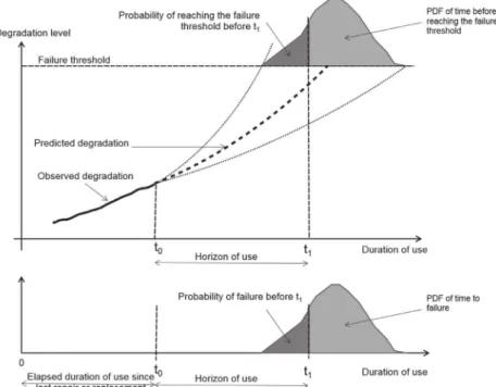
In the domain of PHM, the prognostic activity consists of the ac-curate assessment of the RULs of components of a system[3,9]. This mainly consists in assessing, with a given probability, the duration of use of a component before it fails as this is illustrated inFig. 1where t0
is the current duration of use of the component[5]. In this case, the local prognosis ideally provides a Probability Density Function (PDF) or a Cumulative Probability Distribution Function (CPDF) like in[6–8,10]. If, for different possible reasons (place, weight, cost…), there is not any local prognosis, PDF or CPDF of component failure depending on its uses (duration or number of cycles) can be exploited. These PDFs and CPDFs can be obtained thanks to statistical studies led by the compo-nent suppliers in order to define the probabilities of elementary failures [48], the MTTF and the MTBF of the components. These two situations are illustrated for PDFs inFig. 2where t0is the current duration of use,
and also the date at which the local prognosis is computed, andt1−t0is the duration of the planned tasks.
In these two situations, the probability of failure before t1, noted
pF(t1), can be determined knowing that the probability of reaching the
failure threshold is considered as a failure. Therefore, considering the frame of discernment of a local prognosisP={ ,F F}made of the two states: F that stands for failed and F that stands for not failed, the distribution of bbas on the elements of 2P= ∅ F{ , { }, { }, { ,F F F}} is dogmatic. Let us note that, when bba(ɛ) is time dependent, it is noted bbaɛ(t) where t is the time at which this bba is considered. But the
no-tation bba(ɛ) is also be used when all the bbas are considered at the same time. Therefore, the dogmatic distribution is:bba{ }F ( )t1 =p tF( )1,
= −
bba{ } 1F( )t 1 p tF( )1,bba{ , } 1F F ( )t =0.
However, the probability of failure cannot always be computed for a given duration of use from the data the local prognosis provides. Indeed, the local prognosis can provide data with epistemic un-certainty. The local prognoses can provide two kinds of data containing epistemic uncertainty. The first kind of data consists of an interval varying with the duration of use in which the probability of failure is with a trust α such as the results presented in[22]. This interval can be defined by an upper CPDF and a lower CPDF as shown inFig. 3where plowF(t1) denotes the lower probability of failure before t1with an error
probabilityα2 computed by the local prognosis at t0and pupF(t1) denotes
the upper probability of failure before t1 with an error probabilityα2
computed by the local prognosis at t0too. Therefore, the distribution of
bbas on the elements of 2P is: bba ( )t =p ( )t − −
F lowF α { } 1 1 12 , = + − bbaF ( )t p ( )t α upF { } 1 1
2 1,bba{ , } 1F F ( )t =pupF( )t1 −plowF( )t1 + −1 α. The second kind of data consists of an interval the local prognosis assesses at t0noted [RULmin, RULmax] in which the real RUL is with the
given probability α[4,12,14,32]. Without any other indication about the distribution of the RUL, three situations are considered.
•
The first situation is whent1−t0<RULminfor which the proposeddistribution of the bbas on the elements of 2P is bba ( )t =0 F
{ } 1 ,
=
bba{ } 1F( )t α,bba{ , } 1F F( )t = −1 α. Indeed, as the probability of
oc-currence of the failure between RULminand RULmax is α, thus the
maximum probability of failure before RULminis1− αbut it may be
less because of the lack of information about the distribution of the RUL (this is translated by the bba assigned to{ ,F F}) and so the minimum probability of the non–occurrence of failure before RULminis α.
•
The second situation is whent1−t0>RULmax for which thepro-posed distribution of the bbas on the elements of 2Pisbba ( )t =α F
{ } 1 ,
=
bba{ } 1F( )t 0,bba{ , } 1F F ( )t = −1 α. Indeed, as the probability of
oc-currence of the failure between RULminand RULmax is α, thus the
minimum probability failure will occur beforet1>RULmax+t0 is α but it may be more because of the lack of information about the distribution of the RUL (this is translated by the bba assigned to
F F
{ , }) and so the minimum probability of the non–occurrence of failure before RULminis α.
•
The third situation is whenRULmin≤ −t1 t0≤RULmaxfor which theproposed distribution of the bbas on the elements of 2P is
=
bba{ }F ( )t1 0,bba{ } 1F ( )t =0,bba{ , } 1F F ( )t =1. Indeed, the probability
of occurrence of the failure between RULminand RULmaxis α. This
explains the bba assigned to{ ,F F}is at least α. Nevertheless, the probability the failure occurs outside the interval [RULmin, RULmax]
is1− αbut, because of the lack knowledge about the distribution of the RUL, it is not possible to have an idea of how to distribute this remaining bba between the states F andF. This also corresponds to an epistemic uncertainty between the states F andF. That is why the
remaining belief mass1− αis also assigned to{ ,F F}.
Table 2summarizes the distributions of the bbas on the frame of discernment 2P
of a local prognosis according to the identified types of data provided by the local prognostics.
Local prognoses with epistemic uncertainty seem to be very pena-lizing for the assessment of the future reliability. Nevertheless, the as-sessments of intervals with very high trust α improve the belief inF state although they increase the widths of the intervals. Many works show that these widths are decreasing when t0, the date at which the
local prognoses are computed, is getting close to the date at which
failures occur[4,12,14,22,32].
To assess at t0the multicomponent system ability to carry out the
planned productive tasks that will end at tethe local prognostics must
be computed from the duration the planned tasks will solicit the com-ponents in order to define the values of t1. for the local prognoses.
Nevertheless, the duration of use is not always the best indicator for RULs. Indeed, in some cases the number of cycles is more relevant [7,14,32]. In these cases, the duration of use must be converted into number of cycles. The local prognoses may also require the severity with which the planned tasks will solicit the components that may be introduced thanks to parameters[14]. The durations of uses and the severities can be anticipated by production planning that assigns tasks to systems. Once the local prognoses are determined, the data they provide are used to define their distributions of bbas at teon 2P
ac-cording toTable 2. Therefore, a local prognosis:
•
that is of probability type contains the value of pF(te),•
that is of interval of probability type contains the values pupF(te),plowF(te), and α,
•
that is of trust interval type contains the values RULmin, RULmaxandThe next stage consists in computing the decision supports for production and maintenance planning from the bbas of each set of the power set of the frame of discernment of each entity of the modeled multicomponent system. This computation requires the modeling of the multicomponent system and the definition of inferences. Then in order to simplify the notations, the terms t1and teare not used any more.
Indeed, all the quantities are computed for the date teat which the
Fig. 2.PDFs of the predictions of degradations and of the time to failure.
Fig. 3.Distribution of bbas defined from upper CPDF and a lower CPDF of failure.
Table 2
Distributions of the bbas according to data provided by the local prognosis.
Distribution at t1of bbas on 2P Probability Interval of probability Trust interval
− <
t1 t0 RULmin RULmin≤ −t1 t0≤RULmax t1−t0>RULmax
= bba{ }F ( )t1 pF(t1) plowF( )t1 −1−2α 0 0 α = bba{ } 1F( )t 1− p tF 1( ) 1+α−pupF( )t 2 1 α 0 0 =
planned productive tasks will end.
4. Multicomponent system modeling and inferences
Systems engineering aims at designing technical systems that im-plement specified services and satisfy constraints and desired perfor-mances at lower costs[49]. That is why, the design of a prognostic function for a multicomponent system should be considered at the de-sign stage [33]. Model Based Systems Engineering (MBSE) provides modeling supports for systems engineering such as SysML (System Modeling Language)[50]. The different diagrams enable the identifi-cation of relationships between components, functions and data, energy and material flows. Diagrams, like parametric, sequence, and state-machine diagrams in SysML, model dynamic behaviors of the systems. These models gather structural, functional and behavioral knowledge necessary to implement a prognostic function for a system[30]. The functional knowledge can be extracted from the hierarchical view which breaks down a system into subsystems, then into functions, then into multiple levels of sub-functions till components implementing one or more sub-functions[49]. The structural knowledge is obtained from the direct interactions between entities (components or functions) and their failure modes mainly in order to propagate their effects[51]. For this purpose, MBSE diagrams can be used like, with SysML, the internal blocks diagrams, activity diagrams that represent material, energy and data flows that are used, produced, transformed and exchanged by functions and components. In the present context, the behavioral knowledge can be used to detect degradations of components and to analyse their trends to provide the local prognoses. Data acquisition and data processing techniques implemented for the local prognoses of the components or of their failure modes are numerous and often de-pend on the components or on the failure to prognose[3]. That is why we here consider that the suppliers provide the prognostic systems of their components for their different failure modes. Indeed, they know the behavioral models and they can so implement the most relevant techniques[31]. Therefore, a supplier can provide either one prognosis for each failure mode of the component or one prognosis for all its failure modes. In this last case, the component is assumed having only one failure mode[16].
The modeling proposed in[31]is based on object oriented BN and can be defined from MBSE diagrams. Nevertheless, the obtained graph modeling the multicomponent system must be checked and trans-formed. The first transformations lead to suppress graph cycles, because BNs are acyclic graphs. The second transformations deal with the fact that several paths may exist from a given vertex to another vertex. Those paths can be the consequence of a modeling based on MBSE diagrams such as activity diagrams. The existence of several paths from a vertex E1 to a vertex E2 introduces several times the occurrence probability of one state SE1of E1 into the computation of the occurrence
probabilities of the states of E2 whereas it is a unique occurrence that must so be considered once. The proposed transformations lead to es-tablish several graphs to assess the future reliability of the entities of the system (components, functions, subsystems) whatever their hier-archical levels are. In the resulting modeling graphs, three kinds of
vertices corresponding to patterns appear: components, simple func-tions and redundancy funcfunc-tions for which Bayesian inferences are proposed. These Bayesian inferences only handle aleatory uncertainty. In order to handle epistemic uncertainty too, the proposal consists in adapting, to this modeling, the implementation of the DST by the use of BN inferences for reliability analysis of complex systems proposed in [46,47]and in developing the inferences to take the additional states into account. The main objective is more to define the entities, what-ever their level in the system breakdown structure (from components to subsystems), that will or will not be able to carry out the planned tasks than to identify the operating mode (degraded or not) at the end of these tasks. The handling of epistemic uncertainty of local prognoses leads to a generalization of the method proposed in[31].
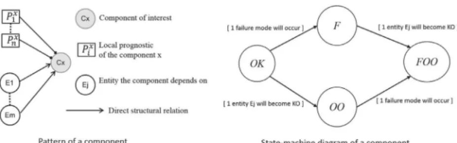
4.1. Component pattern
Assuming components do not have self-healing ability: once they become failed they cannot recover from their failures without main-tenance. According to CBM and PHM policies, maintenance of compo-nents is done before their failures, the case for which the consequence of a component failure could impact the physical integrity of other components, like a leak of a liquid on electrical devices or mechanical structure failure ejecting debris to other components, is therefore not considered. Nevertheless, a component becomes inoperative if another entity, on which it structurally depends, becomes inoperative or fails. That is why the distinction between the inability to operate because of an internal failure and because of another inoperative entity supports the decision making about the components that must undergo main-tenance.
As shown inFig. 4, the pattern of a component is made of a vertex to which one local prognostic at least is connected and that may structu-rally depends on one or several entities. Four distinct states are con-sidered. They define the frame of discernment for a component
=
C {OK F OO FOO, , , }:
•
OK: The component will be able to carry out the planned tasks even if its performances are not the best ones because of incipient de-gradations or of more important dede-gradations.•
F: The component will not be able to operate within its minimum performances required to carry out the planned tasks because at least one internal failure has occurred or will occur. The component will have to undergo maintenance to operate within its minimum performances again.•
OO: The component will not able to operate within the minimum performances required to carry out the planned tasks because at least one entity it structurally depends on is inoperative or will become inoperative. The maintenance of the component is not ne-cessary.•
FOO: The component will not be able to operate within its minimum performances required to carry out the planned tasks because at least one internal failure has occurred or will occur and because at least one entity on which it structurally depends on is inoperative or will become inoperative.=
the frame of discernmentCr={{OK},KOr}. The distribution of bbas on ∈ = ∅ OK KO OK KO
ɛCjr 2Cr { , { }, r, {{ }, r}} are computed from the dis-tribution of bbas onɛiCthe elements of 2Cby the relationship(4)derived
from the Bayesian approximation [52]. Knowing that the fused ele-ments are here chosen a priori and not selected from the values of their bbas, this is not really an approximation.
= ⎧ ⎨ ⎪ ⎩ ⎪ = ∩ = ∅ ∑ = ∑ − ≠ ∅ ⊆ ∩ ≠∅ − = − bba bba KO bba KO bba KO (ɛ ) (ɛ ɛ ɛ ), ɛ (ɛ ), ɛ (ɛ ), ɛ j C i C i C j C j C r KO iC Cj r KO KO KO iC Cj r ɛ ɛ , ɛ ɛ r r r i C r r i C r i C r j Cr r r (4) The distribution of bbas on the elements of 2Cis computed step by
step by the means of inference grids and of the relation(3)by succes-sively considering, on one hand, the local prognostics and, on the other hand, the entities the component depends on. The inference grids are defined from the transitions described in the state-machine diagram of Fig. 4.
The first step consists of a projection of the power set of the frame of discernment 2P = ∅ F{ , { } , { } , { ,F F F} }
1 1 1
1 of the first local prognostic
onto the power set of the frame of discernment 2Cof the component by
setting bba2 ({OK})= bba2 ({ } )F 1 C P1 , bba2 ({ })F = bba2 ({ } )F 1 C P1 and = bba2 ({OK F, }) bba2 ({ ,F F} ) 1
C P1 ; the other bbas of elements of 2Care
set to zero. If the component has more than one local prognostic, the second step consists in considering the impact of the other local prog-nostics one by one thanks to the inference grid ofTable 3and the re-lation (3). In Table 3, the index i denotes the ith considered local prognostic, the indexi−1is for the elements of 2Cwhose values of bbas
do not take into account the bbas of the ith local prognostic yet and the index i is also for the elements of 2C
whose values of bbas are modified once the inference is processed for the ith considered local prognostic. The bbas values of the elements of 2Cnot listed in theTable 3are not
modified.
If the component has entities it depends on, the third step consists in considering the impact of those entities one by one thanks to the in-ference grid ofTable 4and the relation(3). For the jth entity on which the component depends, the power set of the frame of discernment is
= ∅ OK KO OK KO 2E { , { } , { } , { , } }
j j j
j . The state KO means the entity will
not be able to operate within its minimum performances required to achieve the planned tasks whatever the causes are. InTable 4, the index
−
j 1is for the elements of 2Cwhose values of bbas do not take into
account the bbas of2Ejyet and the index j is also for the elements of 2C
whose values of bbas are modified once the inference is processed for
the jth considered entity.
According to the inferences presented in Tables 3 and 4, =
bba2C({OK FOO, }) 0because it is not a result of any inference. This is consistent because the state FOO cannot be reached without passing through the state F or the state OO.
Once the bbas of the elements of 2Care computed, the measures of
belief and plausibility of each element of C are computed from(1)and (2). Then C is reduced to Crby the using(4)for propagation purpose in
the modeling graphs. 4.2. Redundancy pattern
Redundancies are entities that bring into operation the same service or function to match reliability or safety requirements[48]. In many cases, the service is carried out while one entity at least is able to provide it. These cases correspond to parallel structures in reliability diagrams. Particular systems also exist in which the service of re-dundant entities is down if the number of entities that bring it into operation goes under a number p over the n entities that are potentially able to carry it out[46,53]. Nevertheless, it is interesting to distinguish one more state than the one for which the service is operational and the one for which the service is down. This additive state is the one for which the service is operational with the minimum number of re-dundant entities. In such a situation, the system must not begin a new task mainly because of safety reasons[54]. Indeed, the loss of another entity will lead to the loss of the service. Thus maintenance is led before this “loss of redundancy” if the safety criterion is not satisfied.
As shown inFig. 5, the redundancy pattern is made of a vertex to which n entities belong. The n entities carry out the same service that is operative if at least p entities are operative (p < n).
Three distinct states are considered among which one is dedicated to the “loss of redundancy”. They define the frame of discernment for a redundancyRp={OK LR KO, , }.
•
OK: Thanks top+1entities, at least, the service will be operative within the minimum required performances to carry out the planned tasks.•
LR: Only p entities will be operative within the minimum required performances to carry out the planned tasks. Maintenance can be required for safety reasons.•
KO: Less than p entities will be able to operate. This is not sufficient to ensure the minimum performances required to carry out the planned tasks. Maintenance is required to restore the service. Table 3Inference grid for considering more than one local prognostic. 2C 2Pi {F}i { }Fi { ,F F}i − F { }i 1 {F}i {F}i {F}i − OK { }i 1 {F}i {OK}i {OK, F}i − OK F { , }i 1 {F}i {OK, F}i {OK, F}i Table 4
Inference grid for considering the entity the component depends on. 2C
2Ej
{OK}j {KO}j {OK, KO}j
− OK
{ }j 1 {OK}j {OO}j {OK, OO}j
− F
{ }j 1 {F}j {FOO}j {F, FOO}j
− OO
{ }j 1 {OO}j {OO}j {OO}j
− FOO
{ }j 1 {FOO}j {FOO}j {FOO}j.
− OK F
{ , }j 1 {OK, F}j {OO, FOO}j {OK, F, OO, FOO}j
− OK OO
{ , }j 1 {OK, OO}j {OO}j {OK, OO}j
− OK FOO
{ , }j 1 {OK, FOO}j {OO, FOO}j {OK, OO, FOO}j
− F OO
{ , }j 1 {F, OO}j {OO, FOO}j {OO, FOO}j
− F FOO
{ , }j 1 {F, FOO}j {FOO}j {F, FOO}j
− OO FOO
{ , }j 1 {OO, FOO}j {OO, FOO}j {OO, FOO}j
− OK F OO
{ , , }j 1 {OK, F, OO}j {OO, FOO}j {OK, F, OO, FOO}j
− OK F FOO
{ , , }j 1 {OK, F, FOO}j {OO, FOO}j {OK, F, OO, FOO}j
− OK OO FOO
{ , , }j 1 {OK, OO, FOO}j {OO, FOO}j {OK, OO, FOO}j
− F OO FOO
{ , , }j 1 {F, OO, FOO}j {OO, FOO}j {F, OO, FOO}j
− OK F OO FOO
{ , , , }j 1 {OK, F, OO, FOO}j {OO, FOO}j {OK, F, OO, FOO}j
As shown in Fig. 4, there is no direct transition between the state OK and FOO meaning that a failure of the component occurs and an entity Ej becomes KO simultaneously. This transition is neglected because only
the computed quantities, mainly the bbas of the four states, at the end of the planned task te are of interest whatever the order of transitions is.
A fifth state KOr is considered. KOr is the union of the states F, OO
and FOO such as KOr {F, OO, FOO}. KOr means that the component
will not be able to operate within its minimum performances required to achieve the planned tasks whatever the causes are. This state is used to assess the impact of the inability of the component to carry out the planned tasks into the system by propagation in the modeling graphs. For this purpose, it is necessary to reduce the frame of discernment C to
LRcan be seen as a degraded OK state. A state OKris so considered.
OKris the union of the states OK, and LR such asOKr={OK LR, }. This
state is used to propagate, in the modeling graphs, the redundant structure ability to operate within the minimum required performances to carry out the planned tasks. For this purpose, it is necessary to reduce
the frame of discernment Rp to the frame of discernment
=
Rrp {OKr, {KO}}. The distribution of bbas on the elements ∈ = ∅ OK KO OK KO
ɛj 2 { , , { }, { , { }}}
R R
r r
rp rp is computed from the
dis-tribution of bbas onɛiR p
the elements of2Rp
by the relationship(5) de-rived from the Bayesian approximation like(4)for components[2].
= ⎧ ⎨ ⎪⎪ ⎩ ⎪ ⎪ = ∩ = ∅ ∑ = ∑ − ≠ ∅ ⊆ ∩ ≠∅ − = − bba bba OK bba OK bba OK (ɛ ) (ɛ ɛ ɛ ), ɛ (ɛ ), ɛ (ɛ ), ɛ j R i R iR j R j R r OK iR j R r OK OK OK iR j R r ɛ ɛ , ɛ ɛ rp p p rp rp i Rp r p rp iRp r iRp r Rrj p r p rp (5) The distribution of bbas on the elements of2Rpis computed step by
step by the means of inference grids and the relation(3)by successively considering the entities that belongs to the redundancy. The inference grids are defined from the transitions described in the state-machine diagram ofFig. 5.
For 1/n redundancies, the first step consists of a projection of the
power set of the reduced frame of discernment
= ∅ OK KO OK KO 2E { , { } , { } , { , } }
1 1 1
1 of the first entity onto the power set
of the frame of discernment 2R1
of the redundancy by setting = bba2 ({OK}) bba2 ({OK} ) 1 R1 E1 , bba2 ({KO})= bba2 ({KO} ) 1 R1 E1 and = bba2 ({OK KO, }) bba2 ({OK KO, } ) 1 R1 E1
; the bbas of the other elements of2Rpare set to zero. The second step consists in considering the impact
of the states of the other entities one by one thanks to the inference grids ofTables 5and6and the relation(3). InTables 5and6, the index kdenotes the kth considered entity, the indexk−1is for the elements of2R1whose values of bbas do not take into account the bbas of the kth
considered entity yet and the index k is also for the elements of2R1
whose values of bbas are modified once the inference is processed for the kth considered entity. The inference of Table 5 is used for the second entity of the redundancy. Then, the inference ofTable 6is used for all the other entities of the redundancy. The values of the bbas of the elements of2R1not listed in theTable 5are not modified.
For redundancies that need more than one element to be operative (p > 1), a table is built that gives the conditional bbas of the elements of the power set of the frame of discernment2Rpis defined according to
the state-machine diagram ofFig. 5and to the example proposed in [46]for a 2/3 redundancy. Table 7is an excerpt from the complete table defined for a 2/4 redundancy.
Once the bbas of the elements of2Rpare computed, the measures of
belief and plausibility of each element of Rpare computed from(1)and
(2). Then Rpis reduced toR
rpby the using(5)for propagation purpose
in the modeling graphs.
In the case of passive redundancies, the proposed inferences are Fig. 5.Pattern and state-machine diagram of a redundancy.
Table 5
Inference grid for considering the second entity of a redundancy ifp=1.
2R1 2E2
{OK}2 {KO}2 {OK, KO}2
{OK}1 {OK}2 {LR}2 {OK, LR}2
{KO}1 {LR}2 {KO}2 {LR, KO}2
{OK, KO}1 {OK, LR}2 {LR, KO}2 {OK, LR, KO}2
Table 6
Inference grid for considering the entities of a redundancy from the 3rd one to nth one ifp=1.
2R1 2Ek
{OK}k {KO}k {OK, KO}k
− OK
{ }k 1 {OK}k {OK}k {OK}k
− LR { }k 1 {OK}k {LR}k {OK, LR}k − KO { k 1} {LR}k {KO}k {LR, KO}k − OK LR
{ , }k 1 {OK}k {OK, LR}k {OK, LR}k
− OK KO
{ , }k 1 {OK, LR}k {OK, KO}k {OK, LR, KO}k
− LR KO
{ , }k 1 {OK, LR}k {LR, KO}k {OK, LR, KO}k
− OK LR KO
{ , , }k 1 {OK, LR}k {OK, LR, KO}k {OK, LR, KO}k{OK, KO}new
Table 7
Excerpt of the table used to compute the conditional bbas for a 2/4 redundancy.
2E1 2E2 2E3 2E4 2R2
{OK} {OK} {OK} {OK} {OK}
{OK} {OK}
{OK, KO} {OK}
{KO} {OK} {OK}
{KO} {LR}
{OK, KO} {OK, LR}
{OK, KO} {OK} {OK}
{KO} {OK, LR}
{OK, KO} {OK, LR}
{KO} {OK} {OK} {OK}
{KO} {LR}
{OK, KO} {OK, LR}
{KO} {OK} {LR}
{KO} {KO}
{OK, KO} {LR, KO}
{OK, KO} {OK} {OK, LR}
{KO} {LR, KO}
{OK, KO} {OK, LR, KO}
{OK, KO} {OK} {OK} {OK}
{KO} {OK, LR}
{OK, KO} {OK, LR}
{KO} {OK} {OK, LR}
{KO} {LR, KO}
{OK, KO} {OK, LR, KO}
{OK, KO} {OK} {OK, LR}
{KO} {OK, LR, KO}
{OK, KO} {OK, LR, KO}
{KO} {OK} {OK} {OK} {OK}
Two distinct states are considered for a function. They define the frame of discernment for a functionFct={OK KO, }.
•
OK: The function will be able to carry out the planned tasks within the minimum required performances.•
KO: The function will not be able to carry out the planned tasks within the minimum required performances because one of its en-tities, at least, is KO or will become KO during the achievement of the tasks.The distribution of bbas on the elements of2Fct
is computed step by step by the means of an inference grid and the relation(3)by succes-sively considering the entities that belongs to the redundancy. The in-ference grid is defined from the transition described in the state-ma-chine diagram ofFig. 6.
The first step consists of a projection of the power set of the reduced frame of discernment2E = ∅ OK{ , { } , {KO} , {OK KO, } }
1 1 1
1 of the first
en-tity onto the power set of the frame of discernment2Fctof the function by
setting bba2 ({OK})= bba2 ({OK} ) 1 Fct E1 , bba2Fct({KO})= bba2 ({KO} ) 1 E1 and bba2 ({OK KO, })= bba2 ({OK KO, } ) 1
Fct E1 . If more than one entity
contributes to the function, the second step consists in considering the impact of the states of the other entities one by one thanks to the in-ference grid ofTable 8and the relation(3). The index i denotes the ith considered entity, the indexi−1is for the elements of2Fct
whose values of bbas do not take into account the bbas of the ith considered entity yet
and the index i is also for the elements of2Fct
whose values of bbas are modified once the inference is processed for the ith considered entity.
Once the bbas of the elements of2Fct
are computed, the measures of belief and plausibility of each element of Fctare computed from(1)and
(2).
4.4. Computation of the decision support indicators
Once the system is modelled, the obtained graph has to be trans-formed to suppress graph cycles and then this transtrans-formed graph is processed in order to avoid that the bbas of a power set of a unique frame of discernment could be considered several times according to the method described in[31]. This processing may lead to a system modeling made of several graphs for different hierarchical levels of entities. The computation of the decision support indicators can begin when all the local prognoses are obtained for te, the date at which the
planned productive tasks will end.
However, the bbas, Bels and Pls are measures at the credal level. Even if they are relevant to propagate local prognoses epistemic un-certainties in the system ability analysis to carry out production tasks, they can be difficult to handle for decision-makers. The pignistic transformation defines a measure that can be considered as a prob-ability distribution[44]. For each vertex, the pignistic probabilities (BetP) of the elements of its frame of discernment and of its reduced frame of discernment are computed according to(6).
∑
= ∩ ∈ BetP ω( ) bba(ɛ) ω ɛ ɛ i i ɛ 2Ω (6)Considering the computed values of BetP for relevant vertices for te
(those vertices may correspond to solicited system essential entities, mainly functions or sub-systems, for a given sequence of tasks), the decision-makers can valid the sequence of planned productive tasks, reduce the number of tasks, replace or suppress tasks that will solicit too weak functions and, so, plan the needed maintenance operations. To identify the needed maintenance operations and to plan them in terms of time and resources, the identification of components that should undergo maintenance must be done. Thus two more fields are computed for each vertex. The first one is the identifier of the compo-nent whose maintenance will best improve the ability of the vertex to achieve the planned tasks. If the vertex is a component, it can be its own identifier. The second field contains a value computed from the bbas of the power sets of the frames of discernment of entities belonging to the vertex or which the vertex structurally depends on. This field avoids back traversals in graphs. The proposed computation of these two fields is derived from the one presented in[31]. The probability of failure is replaced by the pignistic probability of failure. Thus the computation of these fields, respectively idExandBetP ( )F
maxEx for an entity Ex, becomes,
with Ei and Ek other vertices, BetPEx(ω
i) the pignistic probability of the
state ωiof an entity Ex,Γ (−1Ex)the set of predecessors of Ex and R the
set of vertices that are redundancies in the processed modeling graph: Fig. 6.Pattern and state-machine diagram of a function.
Table 8
Inference grid for considering more than one entity in a function.
2Fct 2Ei
{OK}i {KO}i {OK, KO}i
− OK
{ }i 1 {OK}i {KO}i {OK, KO}i
− KO
{ }i 1 {KO}i {KO}i {KO}i
− OK KO
{ , }i 1 {OK, KO}i {KO}i {OK, KO}i
pessimistic. Indeed, they consider that all the entities ensuring the service will operate together during the planned tasks whereas only one (or the minimum necessary group) will be solicited with the optimistic hypothesis. However, entities ensuring passive redundancies are mainly solicited when all the other entities ensuring the service are failed. In this situation the redundancy is in LR state. Such a situation is often critical in terms of safety and requires urgent maintenance that leads to stop the productive task as soon as possible. This is the case when the ram air turbine must be used in an aircraft, it provides the sufficient energy for control surfaces and some instruments to land urgently [48]. Of course, the programed flight is uncompleted. That is why the values of Bel(LR) and Pl(LR) for a redundancy are, at least; as important as the values of Bel(KO) and Pl(KO) for making decision about production or maintenance.
4.3. Function pattern
Functions can be identified from the hierarchical view. They are implemented by several entities, which can be sub-functions, compo-nents or services brought into operation by redundant entities; but it can also be implemented by a unique entity. A function will fail at achieving the planned tasks as soon as one of the entities implementing it will become inoperative. This is modeled by the means of a serial structure in reliability diagram. Therefore, the function pattern is made of a vertex to which n entities contribute to its implementation as shown in Fig. 6.
•
for a vertex Ex that is a component, the computation ofBetPmaxEk ( )F and idEkis:IfBetPmaxEk ( )F >BetPEx( )F where Ek is such as
= ⎧ ⎨⎩ ⎫⎬⎭ ← ← ← ← ∈ − ∉ ∈
BetP F BetP F BetP KO Then
id id BetP F BetP F Else id Ex BetP F BetP F End if
( ) max max( ( )), max( ( ))
( ) ( ) ( ) ( ) maxEk Ei Ex Ei R max Ei Ei R Ei Ex Ek maxEx maxEk Ex maxEx Ex Γ 1( ) (7)
•
for a vertex Ex that is a redundancy or a function, the computation ofBetPmaxEk ( )F and idEkis:idEx
← idEk ←
BetPmaxEx ( )F BetPmaxEk ( )F (8)
•
where Ek is such as BetPmaxEk ( )F =∈− ∉ BetP F ∈ BetP KO
maxEi Γ1(Ex){maxEi R( maxEi ( )), maxEi R( Ei( ))}
This first approach is justified by the fact that, if the pignistic probabilities of failure were computed for all the local prognoses, the
computations based on object-oriented BN proposed in[31]could be exploited but with the loss of the information about epistemic un-certainties. Other criteria can be used to define components to maintain such as maintenance costs[27]. If failures might lead to casualties or to serious damage to the environment, the plausibility measures of KO and Fstates could be more relevant indicators to define the ability of the main functions to complete the planned tasks as well as to identify the needed maintenance. Thus the process to identify the components to maintain must be adapted to the company's policy declined in terms of reliability, safety, costs, productivity…
5. Experimental results
The proposed method to assess the ability of a multicomponent system to achieve the planned productive tasks has been implement by the means of the discrete event systems simulation Arena software in which the patterns have been defined as blocks. To validate the patterns and the associated computations, the models of a bridge system, of a small system made of 3 components associated in a 2/3 redundancy and of the Kamat–Riley system proposed in[46]have been implemented. For those implementations, the components have had only one local prognosis whose bbas have been initialized with the bbas values of the corresponding components of these models, the function patterns cor-respond to AND gates and the 1/n redundancy patterns to OR gates. The results obtained for the reduced frames of discernment by the proposed Fig. 7.Fictitious system from a systems engineering point of view and its modeling graph.
assessment method have been the same as the ones presented in[46]. The implementation of the system proposed in[31]by its three mod-eling graphs has also been done to validate the identification of com-ponents to maintain. For this validation, all the local prognoses have been initialized with dogmatic distributions of bbas corresponding to the scenarios proposed in [31]for the different scenarios. Therefore, there has been no epistemic uncertainty and so, for all the vertices whose frames of discernment were Ω with ɛi∈2Ω,bba (ɛ ɛi i ≠1)=0.
The bbas, obtained for the models and the scenarios have been the same as the probabilities of the corresponding states as well as the suggested components to maintain.
The fictitious multicomponent system is also the one proposed in [31]. This system is presented onFig. 7.Fig. 7(a) shows the system from a systems engineering point of view andFig. 7(b) shows the modeling graph directly obtained fromFig. 7(a). OnFig. 7(b), the local prognoses of components are shown. This modeling graph is not acyclic and several paths exist between some vertices and requires transformations for the reasons presented inSection 4.4.
Once the transformations described in [31] are done, the three modeling graphs shown onFig. 8are obtained and used for the com-putation of the decision support indicators. In these graphs, the Fncti
stand for functions that are introduced to solve the graph cycles, theFpcts
stands for functions that are considered as subsystems from a systems engineering point of view and FctSstands for the whole fictitious system.
The graph ofFig. 8(a) is used to compute the decision support in-dicators for all the entities of the graph. The graph ofFig. 8(b) is then used to compute the decision support indicators of subsystemsFcts
2 and
Fcts
3 . Eventually, the graph ofFig. 8(c) is used to compute the decision support indicators of the whole system. Four scenarios have been computed from the graphs of Fig. 8. Their results are presented in Table 9where the pignistic probabilities of the frames of discernment are given as well as the identifiers of the suggested components to maintain for each entity. Indeed, we here assume that the decision making process is based, for each entity, on the pignistic probabilities (BetP) of the elements of its frame of discernment that are easier to handle by decision-makers than credal level measures.
The scenario 1 consists of one task lasting(te−t0)4.000 time units
at the end of which all the local prognoses are the same. According to the notations ofSection 3, the local prognoses are supposed pre-pro-cessed and are simulated from the following relationships:
= −
bba{ }F ( )t ek{ }F(t t0) (9)
Ex Scenario 1 Scenario 2 Scenario 3 Scenario 4
BetPEx (LR) BetPEx (KO) idEx BetPEx (LR) BetPEx (KO) idEx BetPEx (LR) BetPEx (KO) idEx BetPEx (LR) BetPEx (KO) idEx
FctS 6.28E-03 C23 1.18E-02 C21 6.48E-03 C21 8.82E-03 C34
Fcts
3 2.70E-03 C32 5.49E-03 C34 3.00E-03 C34 5.49E-03 C34
Fcts
2 3.59E-03 C23 6.38E-03 C21 3.50E-03 C21 3.35E-03 C25
Fcts
1 7.55E-10 C13 3.60E-09 C11 7.06E-10 C11 3.60E-09 C11
Fct
5 1.35E-03 C36 1.55E-03 C37 9.50E-04 C37 1.55E-03 C37
Fct
4 1.35E-03 C36 1.55E-03 C37 9.50E-04 C37 1.55E-03 C37
Fct
3 1.35E-03 C32 3.95E-03 C34 2.05E-03 C34 3.95E-03 C34
Fct
2 2.25E-03 C21 5.04E-03 C21 2.75E-03 C21 2.00E-03 C25
Fct
1 2.25E-03 C23 4.84E-03 C21 2.55E-03 C21 1.80E-03 C23
Fcti
2 1.35E-03 C36 1.55E-03 C37 9.50E-04 C37 1.55E-03 C37
Fcti
1 9.00E-04 C21 3.50E-03 C21 1.80E-03 C21 4.50E-04 C22
R21 9.00E-04 2.03E-07 C33 3.50E-03 1.37E-06 C34 1.80E-03 3.89E-07 C34 3.50E-03 1.37E-06 C34
R11 2.46E-06 7.38E-10 C13 8.04E-06 3.51E-09 C11 2.58E-06 6.57E-10 C11 8.04E-06 3.51E-09 C11
Ex BetPEx (F) BetPEx (KO) idEx BetPEx (F) BetPEx (KO) idEx BetPEx (F) BetPEx (KO) idEx BetPEx (F) BetPEx (KO) idEx
C37 4.50E-04 4.50E-04 C37 6.50E-04 6.50E-04 C37 4.50E-04 4.50E-04 C37 6.50E-04 6.50E-04 C37
C36 4.50E-04 4.50E-04 C36 4.50E-04 4.51E-04 C36 2.50E-04 2.50E-04 C36 4.50E-04 4.51E-04 C36
C35 4.50E-04 4.50E-04 C35 4.50E-04 4.50E-04 C35 2.50E-04 2.50E-04 C35 4.50E-04 4.50E-04 C35
C34 4.50E-04 4.50E-04 C34 3.05E-03 3.05E-03 C34 1.55E-03 1.55E-03 C34 3.05E-03 3.05E-03 C34
C33 4.50E-04 4.50E-04 C33 4.50E-04 4.50E-04 C33 2.50E-04 2.50E-04 C33 4.50E-04 4.50E-04 C33
C32 4.50E-04 9.00E-04 C32 4.49E-04 3.50E-03 C34 2.50E-04 1.80E-03 C34 4.49E-04 3.50E-03 C34
C31 4.50E-04 4.50E-04 C31 4.50E-04 4.50E-04 C31 2.50E-04 2.50E-04 C31 4.50E-04 4.50E-04 C31
C25 9.00E-04 9.00E-04 C25 1.10E-03 1.10E-03 C25 7.00E-04 7.00E-04 C25 1.10E-03 1.10E-03 C25
C24 4.50E-04 1.35E-03 C21 4.48E-04 3.95E-03 C21 2.50E-04 2.05E-03 C21 4.50E-04 9.00E-04 C22
C23 1.35E-03 1.35E-03 C23 1.35E-03 1.35E-03 C23 7.50E-04 7.50E-04 C23 1.35E-03 1.35E-03 C23
C22 4.50E-04 4.50E-04 C22 4.50E-04 4.50E-04 C22 2.50E-04 2.50E-04 C22 4.50E-04 4.50E-04 C22
C21 4.50E-04 4.50E-04 C21 3.05E-03 3.05E-03 C21 1.55E-03 1.55E-03 C21 1.00E-07 1.04E-07 C21
C13 9.00E-04 9.00E-04 C13 9.00E-04 9.00E-04 C13 5.00E-04 5.00E-04 C13 9.00E-04 9.00E-04 C13
C12 9.00E-04 9.00E-04 C12 1.10E-03 1.10E-03 C12 7.00E-04 7.00E-04 C12 1.10E-03 1.10E-03 C12
C11 9.00E-04 9.00E-04 C11 3.50E-03 3.50E-03 C11 1.80E-03 1.80E-03 C11 3.50E-03 3.50E-03 C11
Table 10
Computed and usable quantities to support decision for redundancyR21in scenario 1.
2R21 bba2 2R1(.) Bel2 2R1(.) BetPR21(.) Pl2 2R1(.) 2R r21 Bel2 2R r1(.) BetPR r12(.) Pl2 2R r1(.)
{OK} 9.990E-01 9.990E-01 9.991E-01 9.992E-01 {OKr} 9.999E-01 9.999E-01 9.999E-01
{LR} 7.996E-04 7.996E-04 8.996E-04 9.996E-04
{OK, LR} 1.999E-04 9.999E-01 9.999E-01
{KO} 1.600E-07 1.600E-07 2.033E-07 2.500E-07 {KO} 1.600E-07 2.050E-07 2.500E-07
{LR, KO} 8.000E-08 7.998E-04 9.997E-04
{OK, LR, KO} 1.000E-08 1.000E + 00 1.000E + 00 {OKr, {KO}} 1.000E + 00 1.000E + 00
Table 9
![Fig. 1. Probability densities associated to RUL [5] .](https://thumb-eu.123doks.com/thumbv2/123doknet/2974200.82887/5.892.215.668.886.1125/fig-probability-densities-associated-rul.webp)