Quasi-symmetrical contact algorithm and recurrent boundary conditions: application to 3d metal forging simulations

HAL Id: pastel-00002047

https://pastel.archives-ouvertes.fr/pastel-00002047

Submitted on 11 Jun 2007

HAL is a multi-disciplinary open access archive for the deposit and dissemination of sci-entific research documents, whether they are pub-lished or not. The documents may come from

L’archive ouverte pluridisciplinaire HAL, est destinée au dépôt et à la diffusion de documents scientifiques de niveau recherche, publiés ou non, émanant des établissements d’enseignement et de

boundary conditions: application to 3d metal forging

simulations

Sorin Popa

To cite this version:

Sorin Popa. Quasi-symmetrical contact algorithm and recurrent boundary conditions: application to 3d metal forging simulations. Engineering Sciences [physics]. École Nationale Supérieure des Mines de Paris, 2005. English. �NNT : 2005ENMP1422�. �pastel-00002047�

N° attribué par la bibliothèque |__|__|__|__|__|__|__|__|__|__|

T H E S E

pour obtenir le grade de

Docteur de l’Ecole des Mines de Paris

Spécialité «Mécanique Numérique»

présentée et soutenue publiquement par

M. Sorin POPA

Soutenue le 10 juin 2005

QUASI

-

SYMMETRICAL CONTACT ALGORITHM AND

RECURRENT BOUNDARY CONDITIONS

:

APPLICATION

TO 3D METAL FORGING SIMULATIONS

Directeur de thèse : M. Lionel FOURMENT

Jury :

M. Laurent Baillet

…

Rapporteur

M. José M.A. César de Sá

…

Rapporteur

M. Serge Cescotto

…

Examinateur

M. Richard Ducloux

…

Examinateur

Remerciements

Cette thèse a été effectuée au Centre de Mise en Forme des Matériaux ( CEMEF)de l’Ecole Nationale Supérieure des Mines de Paris. Je voudrais remercier à la direction de l’Ecole des Mines et particulièrement à Monsieur Jean Loup Chenot, qui a dirigé mon stage initial au sein de CEMEF après lequel il m’a proposé le contrat de thèse, malgré mon manque d’expérience dans les domaines de la mise en forme et les mathématiques appliquées.

Cette thèse n’aurait vu le jour sans la confiance, la patience et la générosité de mon directeur de recherche, Monsieur Lionel Fourment, que je veux vivement remercier. De plus, les conseils qu’il m’a divulgué tout au long de la rédaction, ont toujours été clairs et succincts, me facilitant grandement la tâche et me permettant d’aboutir à la production de cette thèse.

Je remercie les rapporteurs de cette thèse, M. Laurent Baillet et M. José M.A. César de Sá pour la rapidité avec laquelle ils ont lu mon manuscrit et l’intérêt qu’ils ont porté à mon travail. Merci également aux autres membres du jury qui ont accepté de juger ce travail, M. Serge Cescotto et M. Richard Ducloux.

Un grand merci pour tout l’équipe de CEMEF pour m’avoir fourni d’excellentes conditions logistiques et financières et tout particulièrement a Monsieur Patrick Coels qui m’a soutenu dans ma démarche personnelle de « regroupement sentimental ».

Mes plus chaleureux remerciements s’adressent à Josué Barbosa, Ramzy Bousetta, Cyril Gruau, Olga Karasseva, Mihaela Teodorescu et tout les autre collègues pour leur soutien moral qu’ils m’ont fourni tout au long de la réalisation de ces travaux.

Cette thèse s’appuie sur deux articles en anglais publiés dans des revues internationales, aussi en proposons-nous une brève introduction.

Cette thèse faisait partie du projet national français Simulforge, qui réunissait plusieurs laboratoires de recherche et partenaires industriels de la forge, ainsi que le Centre technique des industries de la mécanique (CETIM) et Transvalor, l’éditeur du logiciel Forge3®.

Dans la première partie, la thèse traite de la réduction de temps de calcul pour la simulation du forgeage des engrenages hélicoïdaux. Sur la figure 1, on observe que les engrenages hélicoïdaux obéissent à un modèle de répétition. Il est donc possible de simuler le forgeage d’une seule dent. Le chapitre 2 décrit brièvement l’approche numérique du problème thermomécanique du forgeage. Dans le chapitre 3, on s’occupe plus en détails des conditions de symétries nécessaires pour effectuer la simulation du forgeage sur le domaine réduit à une seule dent. Ces conditions de symétries cycliques consistent à imposer que la matière qui sort d’une face de symétrie entre dans l’autre face. Cette condition se traduit par l’identité entre le champ de vitesse (chapitre 3.2) et de températures (chapitre 3.3) sur les deux surfaces de symétrie. Cette condition est très similaire à celle de contact collant entre les corps déformables, si on fait abstraction de la matrice de rotation introduite en sus. Donc, pour imposer cette condition de symétrie, un algorithme de type maître-esclave est nécessaire, semblable à celui utilisé pour traiter le contact entre les corps déformables. Dans le chapitre 3.2 on explique comment on obtient les différentes variables par l’algorithme de contact standard de Forge3® multi-corps, et comment on applique ensuite la condition de symétrie cyclique. Le chapitre 3.4 décrit comment gérer les nœuds qui se trouvent sur l’axe de symétries, nœuds qui peuvent seulement se déplacer sur l’axe. On bloque donc leurs degrés de liberté perpendiculaires à cet axe.

Un problème particulier se pose quand on doit simuler le forgeage avec des outils déformables. A cause de l’approche Lagrangienne utilisée, et éventuellement aussi à cause de la géométrie initiale, la matière d’une dent de la pièce ne sécoule pas forcement dans une seule dent de l’outil. On explique, dans le chapitre 3.5, que multiplier la zone

chapitre 3.6. Elles consistent à écrire le contact entre les parties « libres » de la pièce de l’outil, en utilisant des outils virtuels qui peuvent être multipliés autant de fois qu’il faut pour appliquer complètement les conditions aux limites nécessaires, sans alourdir les calculs.

Le chapitre 4 est consacré à la validation de la méthode. Les premiers tests académiques présentés dans 4.1 montrent que la précision est tout à fait satisfaisante pour une formulation pénalisée du problème de contact. Les temps CPU sont augmentés par rapport à ceux obtenus pour les symétries planes, probablement à cause de la présence des plusieurs termes pénalisés dans les systèmes linéaires, mais la réduction de temps de calcul estimée par rapport une la simulation sur tout le domaine est considérable. Le test industriel offert par Ascoforge, présenté dans le chapitre 4.2, montre une bonne précision globale de l’algorithme durant toute la simulation, précision évaluée en mesurant l’écart entre une surface de symétrie et son image par rotation. Par ailleurs, ce test qui a une cinématique particulière met en évidence l’impossibilité de traiter ce type de problème en utilisant les symétries planes, même si le problème vérifiait effectivement des conditions de symétries planes. Dans le paragraphe 4.3, on présente un exemple de simulation de forgeage avec des outils déformables, ce qui montre la fiabilité globale de la méthode. Comme cette première partie s’appuie sur le contact maître-esclave, la suite évidente de ce travail est d’améliorer cette formulation, dans la deuxième partie de la thèse. Le problème de cette approche est que dans les cas ou le maître est discrétisé plus finement que le corps esclave la précision se dégrade, car il y a des nœuds en contact sans conditions aux limites (voir chapitre 3.1 de la deuxième partie).

Dans le chapitre 2 on présente le problème continu du contact, la formulation faible du problème et la discrétisation éléments finis.

Le chapitre 3 présente plusieurs algorithmes de contact proposés par la littérature. Sans entrer en détails, on montre que l’approche symétrique (3.2) conduit à une formulation sur contrainte du problème. Le raccord intégral (3.3) et les éléments mortar (3.4) donnent des bons résultats en 2D mais en 3D ils sont difficiles á appliquer et potentiellement chers en temps CPU.

d’éviter de sur-contraindre le problème. Au niveau discret, il y a toujours une distinction entre la surface maître et la surface esclave. On intègre l’équation de contact seulement sur la surface esclave, donc cette formulation reste dans le cadre maître-esclave, mais cette fois tous les nœuds des deux interfaces en contact imposent des conditions de contact qui leur sont associées. Le contact quasi-symétrique est implémenté dans le cadre d’une formulation nodale pénalisée.

Le chapitre 4 présente les diverses validations de cette méthode. En 4.1 on s’occupe d’évaluer la vitesse de convergence de cette méthode, en utilisant une famille de maillages emboîtés. La formulation quasi symétrique, ainsi que celle habituelle ont une bonne vitesse de convergence, similaire à celle obtenu avec des maillages coïncidents. En 4.2 on présente un patch test défini sur un maillage non régulier qui ne pose toujours pas de problèmes de consistance pour la formulation standard. Toutefois, en utilisant la formulation maître esclave, on double pratiquement la précision et on voit une amélioration nette du champs de pressions transmis. Le premier test du chapitre 4.3 accentue cette conclusion, et le deuxième test de cette section montre un net avantage en termes de précisons de la formulation quasi-symétrique quand le maillage du maître est plus raffiné que celui de l’esclave. En effet, ce test montre que la précision ne dépend quasiment pas du choix du maître de l’esclave. Le test d’indentation présente dans cette partie est un test extrême de détection du contact qui donne des résultats corrects quand on utilise le contact quasi symétrique, même s’il n’y a pas aucun nœud du corps esclave en contact.

Les cas d’étude industriels proposés par les partenaires de Simulforge sont regroupés dans le chapitre 5. Le première est le forgeage d’une pièce automobile constituée de deux matériaux en contact bilatéral collant et qui sont remaillés plusieurs fois au cours de la simulation du forgeage. Les calculs tournent pratiquement aussi vite avec la formulation quasi-symétrique qu’avec la que la version maître-esclave de base, mais à la fin de la simulation on obtient une bien meilleure qualité des résultats. Cette conclusion est confirmée par le deuxième test industriel, sur lequel on observe visuellement une meilleure distribution de la pression sur la zone en contact. Ces deux teste montrent aussi la stabilité et la fiabilité de l’implémentation.

Les méthodes présentées dans cette thèse se montrent efficaces et fiables. Les symétries de répétition permettent de réduire considérablement le temps CPU pour la simulation du forgeage des engrenages hélicoïdaux, et l’approche quasi-symétrique du contact améliore la précision des simulations multi-corps, et rend le logiciel plus facile a utiliser.

En perspective, l’approche quasi-symétrique peut être utilisé aussi pour traiter les symétries de répétition. Le frottement est un problème encore ouvert. Quelques tests montrent qu’une approche symétrique du frottement donne des bons résultats, mais il est nécessaire d’une étude plus approfondie sur le sujet. Les deux méthodes présentées peuvent également être étendues à d’autres problèmes faisant apparaître ces type de symétries de répétition, comme le fluotournage, et à d’autres méthodes de résolution du contact, comme les formulations intégrées.

INTRODUCTION 1

PART 1 – HELICAL GEAR FORGING SIMULATION USING RECURRENT BOUNDARY CONDITIONS

5

Abstract 7

1. INTRODUCTION 8

2. PROBLEM STATEMENT 9

2.1 Continuous problem 9

2.2 Discrete problem and Algorithm Splitting 13

3. RECURRENT BOUNDARY CONDITIONS 17

3.1 Recurrent condition 17

3.2 Discrete periodicity condition for velocities 18 3.3 Discrete periodicity conditions for temperatures 20

3.4 Node on the symmetry axis 20

3.5 Deformable tools 21

3.6 Algorithm for deformable tools 22

4. APPLICATIONS 24

4.1 Accuracy and time reduction evaluations 24 4.2 Industrial Test. Helical Gear Forging 28

4.3 Gear forging with deformable dies 31

FOR LARGE 3D DEFORMATION SOLID MECHANICS

ABSTRACT 39

1. INTRODUCTION 39

2. DEFORMABLE BODIES: CONTACT FORMULATIONS 40

2.1 Contact equations 40

2.2 Problem statement 41

2.3 Finite element discretization 42

3. CONTACT FORMULATIONS 43 3.1 Master / Slave 43 3.2 Double Pass 44 3.3 Integral joint 45 3.4 Mortar elements 47 3.5 Quasi-symmetric formulation 47 4. VALIDATIONS 49 4.1 Convergence rate 49

4.2 Contact patch test 52

4.3 Qualitative tests 55

4.6 Industrial forging problem 68

5. APPLICATONS 61

CONCLUSION AND PROSPECTS

REFERENCES

67

1. INTRODUCTION

General considerations

The forging industry in Europe had a continuous growth during the last decade, even if the number of forging companies diminished. The companies involved in this competition have a constant need to increase the quality of the products and to decrease the production costs . The traditional design stages of a new product series imply expensive trials, on actual forging machines, which require stopping the production. The tendency is now to replace these tests by virtual, numerical ones. For the moment, the actual trials are not eliminated, but their number has considerably decreased. Using numerical simulation a wide range of mechanical and thermal data can be obtained, allowing the numerical optimization of the forging series, of the required forming energy, allowing to increase the tools life-span and making so possible to understand the reasons why a proposed design is not satisfactory or to improve the current one

Few years ago, numerical simulation was the domain of only few experts having a solid background in mechanics, numerical methods and programming. On the other hand, the computers were expensive and much slower. However, this situation is continuously changing, the computer prices are dropping and the performances are exploding. In the meantime, the software progressed, becoming more and more user-friendly and robust. The first finite element based simulations took place in early seventies. At CEMEF, in 1981 the development of Forge2® started, for running forging simulations on axisymmetrical configurations. The studies for a fully 3D simulation code started in 1983, and in 1991 the first commercial version of Forge3® was launched. This software allows simulating forming processes with large deformations, such as forging, rolling, etc. It has a friendly interface, so numerical tests can be easily created and launched without requiring advanced knowledge of numerical methods. It provides the forming history undergone by the workpiece i.e. strain, stress, temperature, as well as global values such as forging force or energy, stresses on the tools, etc.

The frame of this work

This thesis is a part of a larger project gathering several research laboratories called SIMULFORGE, sponsored by the French government. This project also puts together the efforts of 16 French forging companies, the Technical Center of Mechanical Industries (CETIM) and TRANSVALOR, a company in charged marketing Forge3®.

The purpose of this study is twofold: reducing the required computational time for the forging simulation of helical gears by taking into account the non conventional symmetries of the problem, and improving the contact algorithm between deformable bodies, like the workpiece and the tools in the forging context.

When this research was started, an academic version of Forge3® was available, which was capable of running simulations for multiple bodies problems. The contact between deformable bodies was handled by a Master / Slave algorithm. This formulation was then used in the first part of this study, about the recurrent boundary conditions. So, the first part of this thesis, which is about to be published as an article in the Special Issue of the International Journal of Forming Processes 2004, presents the basics of Forge3®, and the proposed approach to handle this type of boundary conditions. The purpose is to allow running the forging simulation of helical gears (or any such repetitive configurations) only on one tooth of the domain, both for the workpiece and for the dies. The recurrent boundary conditions are regarded as the contact conditions between deformable bodies. Therefore, after acquiring profound knowledge of the contact formulations and algorithms, the question of developing more symmetrical contact algorithms arose. This is the purpose of the second part of this thesis. Part 2 provides detailed description of the quasi-symmetrical contact formulation, and of the several tests, both academical and industrial that have been used to validate and evaluate this new formulation.

SIMULATION USING RECURRENT

BOUNDARY CONDITIONS

recurrent boundary conditions

Sorin Popa1, Lionel Fourment1

1

Cemef - Ecole des Mines de Paris & UMR CNRS n° 7635 B. P. 207, F-06904 Sophia Antipolis Cedex

URL:http://www-cemef.cma.fr/

e-mail: lionel.fourment@ensmp.fr

ABSTRACT. In gear forging simulation, the use of symmetries is obviously an efficient solution

to reduce the computational time. However, for helical gears, standard plane symmetry conditions do not hold. They have to be extended to recurrent boundary conditions where the material flow that leaves one of the symmetry surface re-enters through the symmetric one, which is derived from it by a rotation of 2p/Nteeth radians, (Nteeth is the number of teeth of the

gear). In this case, the symmetry surfaces are not necessarily plane. This paper presents a master-slave algorithm for imposing these conditions, both for velocities and temperatures. It makes it possible to carry out simulations of helical gear forging considering only one tooth. Using a Lagrangian mesh, the symmetry surfaces are not steady during the deformation process, so a special treatment is required to handle the contact with deformable tools in the recurrent frame. Academic tests are studied to evaluate the accuracy of this approach, and then industrial applications show its robustness.

KEYWORDS. recurrent boundary conditions, master-slave algorithm, forging, helical gear, contact between deformable bodies

1. INTRODUCTION

Numerical simulation is an important step of the design process, particularly in forging where its cost is very low compared to industrial experiments. Actual trials require tools manufacturing and stopping industrial production, which all together results in high prices. Moreover, numerical simulation provides extensive information like material flow, tool stresses and life span or elastic spring back, information that are difficult to obtain otherwise. Therefore, it is a very attractive alternative. It also allows process optimisation in a very simple and friendly way, for instance to improve the tool geometries in order to decrease the required energy and increase the tooling life span. However, complex 3D simulations have a significant computational cost that has to be acknowledged and that may reduce its attractiveness. The purpose of this work is to reduce this computational cost for the simulation of helical gear forging (see figure 1) or similar processes, by reducing the problem size taking into consideration the natural symmetries of the process. In fact, it is theoretically possible to study only 2π/Nteeth of the problem, where Nteeth is the number of teeth of the gear. These symmetries are not standard, like plane symmetries. Usually, they are not handled by finite element software, so the entire workpiece has to be considered, which results into very large computational time.

Figure 1. Example of helical gears.

As the process exhibits same symmetries as the gear itself, the material flow is periodic according to a rotation of 2π/Nteeth along the gear axis. It allows considering the material volume of only one tooth. Some authors call this type of boundary conditions “principle of repeatability” or “cyclic symmetry” (Huang et al. 04), or qualify it as recurrent (Park et al. 97). With little modifications, this principle also applies to other types of recurrent boundary conditions, where, for instance, rotation is replaced by translation, as in the forming of a composite material at a micro scale. In (Park et al. 97), the method is presented in the limited frame of a structured mesh with nodes coinciding by rotation of the symmetry surfaces. In (Huang et al. 04), it is extended to unstructured meshes, without any constraint on the mesh, which makes it possible to apply it to both 2D and 3D problems. Here, the

same approach is followed, and is further extended to coupled calculations with deformable tools. This work is developed in the Forge3® finite element software that is based on a P1+/P1, velocity and pressure formulation (Aliaga et al. 98), uses unstructured meshes of tetrahedra and has automatic remeshing facilities (Coupez 94). Next section presents the thermo-mechanical problem and its finite element resolution. Section 3 introduces the recurrent boundary conditions in the frame of a master/slave contact algorithm between deformable bodies. Final section shows numerical simulations of complex gear forging, both with rigid and deformable tools.

2. PROBLEM STATEMENT

2.1. Continuous problem

The problem equations are presented in a rather simplified way for cold forging conditions. More details about the formulation and about more complex material models can be found in (Aliaga et al. 98, Barboza et al. 02, Pichelin et al. 01). The Prandl Reuss additive decomposition of the strain rate tensor ε& is considered:

⎪⎩ ⎪ ⎨ ⎧ = + = −_s L e e e e & & & & & 1 el vp el [1]

where ε& is the elastic part of the strain rate tensor and el ε& the viscoplastic one, σ isvp the stress tensor and σ& its time derivative, L is a 9x9 tensor containing the Lamé coefficients λ and µ :

I e

s& =2µ&+λtr(ε&) [2]

The viscoplastic deformation follows the Norton-Hoff constitutive model. Considering K, the material consistency and m, the strain rate sensitivity coefficient, we have: vp m K pI e s s= + =2 ( 3ε&) −1& [3] 0 ) ( vp = tr e& [4]

p E

div(v)=−3(1−2υ) [5]

where s is the deviatoric stress tensor, E the Young coefficient, υ the Poisson coefficient, ε& the equivalent strain rate, and p the hydrostatic pressure:

) ( 3 1 s tr

p=− and &

(

e&vp:e&vp

)

3

2 =

ε [6]

Neglecting all external forces like gravity and inertia, at any time of the process, the balance and heat equations are written as:

( )

s =0 div [7] e : s & f T grad k div dt dT c_p + ( ⋅ ( ))= ρ [8]

where T is the temperature, cp the heat capacity, k the conductivity, ? the density and f is a conversion rate between 0 and 1 (usually around 0.9).

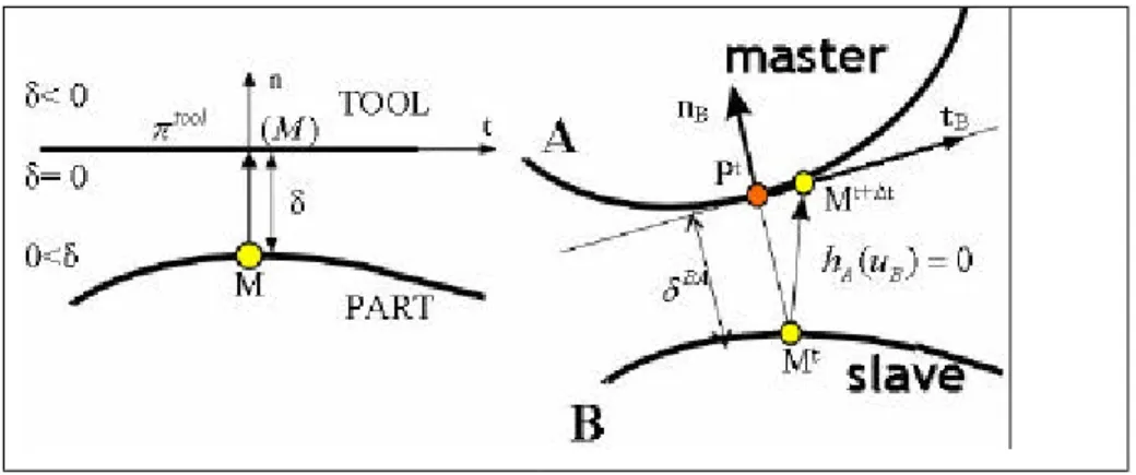
2.1.1 Contact with rigid tools

Figure 2. a) Contact with rigid tool b) Contact between deformable bodies

These equations are complemented by different boundary conditions, such as unilateral contact with the forming tools, or Signorini conditions. Considering <·> as the scalar product, these conditions are written as:

(

)

(

)

[

]

⎪ ⎩ ⎪ ⎨ ⎧ = − ⋅ − ≤ ⋅ = ≤ ⋅ − Ω ∂ 0 0 , on n contact σ δ δ n u u n s n s n u u tool n tool [9]

where u is the displacement vector, utool is the tool one, n is the ingoing normal of the tool surface, nσ is the normal stress vector, and δ is the signed distance to the tool surface (which is negative inside the tool, see figure 2.a). For the contact conditions, displacement unknowns are used while velocity unknowns are preferred elsewhere. Several models can be used for the friction boundary conditions between the workpiece and the rigid tools. Neglecting the gliding threshold, equation [10] gives the Tresca model:

t t v v t ∆ ∆ − − = Ω ∂ 3 , on _friction m σ0 [10] n s s n t = − _n [11]

(

)

(

v v n

)

n v v v = − − − tool ⋅ ∆ t tool [12]

whereτ is the tangential component of the stress tensor on the contact surface, ∆vt

is the relative tangent velocity between the bodies, m is the friction coefficient and

0

σ is the material flow stress.

2.1.2 Contact between deformable bodies

The contact conditions between two deformable bodies A and B (workpiece and deformable tool, for example) are given in [13] when body B is in contact with body A:

[ ]

( )

⎪ ⎩ ⎪ ⎨ ⎧ = ≤ ⋅ = ⋅ = ≤ − ⋅ − = ∂ 0 0 0 ) ( , on B A A A B A B B u n n s n n s n u u u A n B B B n BA A AB h ) ( h O σ σ δ [13]

and also, symmetrically, the inequality h_B(u_A)≤0 could be considered. These equations can be extended to any number of bodies. The friction condition between bodies B and A is written similarly to [10], with:

(

B A B

)

B A B v v v n n v v = − − − ⋅ ∆ _t ( ) ( ) [14]

As for the contact conditions, the friction equation could also be written for the body

A with body B. In anticipation to the equations that will be necessary to handle the

recurrent boundary conditions, we introduce here the bilateral sticking contact equations between deformable bodies:

0 ) (uB =uB−uA− nB = BA A h δ [15]

These boundary conditions are completed with the free surface one: 0

,

on∂Ω_free s n= [16]

2.1.3 Thermal boundary conditions

For the thermal problem, several boundary conditions are applied. Considering hex the convection/radiation coefficient with the air, htool the transfer coefficient with a rigid tool, Tex the air temperature and Ttool the rigid die temperature, the convection/radiation boundary conditions are written as:

( )

ex

(

ex

)

free kgrad T h T T

O − ⋅ = −

∂ , n

on [17]

and a similar equation describes the heat exchange with a rigid tool:

( )

tool

(

tool

)

contact kgrad T h T T

O − ⋅ = −

∂ , n

on [18]

Considering hc the conductivity of the interface, the heat transfer between two deformable bodies is given by:

( )

B c

(

B A

)

A

( )

A c

(

A B

)

B gradT h T T k grad T h T T

k ⋅ = − − ⋅ = −

− n and n [19]

The heat produced by the friction is also considered:

( )

⋅n= t ⋅v

− Ω

∂ friction, kgrad T hfriction

on [20]

where hfriction is a coefficient depending on the effusivities of the two parts in contact. 2.1.4 Plane symmetry

Considering n_sym the outgoing normal of the symmetry plane ∂Ωsym, the following

symmetry boundary conditions are imposed respectively for the mechanical and thermal problems:

0 ,

on∂Ωsym v⋅nsym = [21]

( )

(

gradT

)

sym sym

k ⋅ = ∂Ω

− n 0on [22]

2.2. Discrete problem and algorithm splitting:

2.2.1 Time discretization

Using an updated Lagrangian formulation, an explicit Euler time discretization scheme is chosen for the mechanical problem. Considering t

x the values at time t, the values at time t+∆t can be approximated by:

t t t t t t+∆ _{= x +v}+∆_∆ x [23]

Using this time discretization, the contact boundary conditions are written again at time t+∆t using velocities unknowns [24], so the unilateral contact with the rigid tools is given by [25]. t t t t t t t t+∆ _{= x}+∆ _{−x =v}+∆_∆ u [24] 0 ) ( ≤ ∆ − ⋅ − +∆ ∆ + t t t t t tool t t _{v n} δ v [25]

Similarly, the bilateral sticking contact condition is given by:

0 = ∆ − − +∆ ∆ + t t t t tool t t tn v v δ [26]

From now on, the distances d and dBAas well as the normals n and nb are calculated at time t, so the time indexes are not written any longer. Then, the bilateral sticking and the unilateral contact equations between deformable bodies respectively become: 0 ) ( = ∆ − − = +∆ +∆ B BA t t A t t B B A t h u v v δ n [27]

(

)

0 ) ( ≤ ∆ − ⋅ − = +∆ +∆ t h BA B t t A t t B B A u v v n δ [28]

Concerning the thermal problem, a time discretization scheme with two time steps is used. Without going too much into details, the thermal problem is solved at an intermediate time ti∈

[

t,t+∆t

]

and:

t T T t T T dt dTti t t t t t t ∆ − + ∆ − − =(1 γ ) −∆ γ +∆ [29]

The temperature at time t+∆t are updated using the following equation:

) ( 1 2 3 t t t t t t T T T T i α α α − + = +∆ ∆ + _[30]

where the numerical coefficients α₁,α₂,α₃,γ are given by the Dupont scheme

( , 1 4 3 , 0 , 4 1 3 2 1 = α = α = γ = α ).

Considering an elasto-viscoplastic material, and t t t t

( v , p ,T ,Ω being known, the)

resolution of the thermo-mechanical problem provided by equations [7], [5], [8] and previously described boundary conditions, allows calculating

t t t t t t t t

( v+∆ , p+∆ ,T +∆ ,Ω+∆ ). The mechanical and thermal problems are coupled, as the consistency of the material depends on the temperature, and the heat equation depends on the mechanical solution. A splitting algorithm is used, so the thermo-mechanical problem is decomposed in a thermo-mechanical problem that uses the temperature field of the previous time step, and a thermal problem that uses the calculated mechanical solution.

2.2.2 Finite element formulation

Considering H1t Ω a Sobolev space on t Ω , and L2t Ω a Hilbert space on t Ω , the space of kinematically admissible velocities is defined as:

(

)

( )

(

)

⎪ ⎩ ⎪ ⎨ ⎧ ⎪ ⎭ ⎪ ⎬ ⎫ Ω ∂ = ⋅ Ω ∂ ≤ ∆ − ⋅ − Ω ∂ ≤ ∈ = = Ω Ω sym contact AB A CA t h xH H V t B t A on 0 , on 0 , on 0 , 1 1 sym tool B B A n v n v v v v , v v δ

and the one of the kinematically admissible to 0 as:

(

)

⎪⎩ ⎪ ⎨ ⎧ ⎪⎭ ⎪ ⎬ ⎫ Ω ∂ = ⋅ Ω ∂ ≤ ⋅ Ω ∂ ≤ ⋅ ∈ = = Ω Ω sym t contact AB B t B t B t A t CA H tAxH tB V on 0 , on 0 , on 0 , 1 1 0 sym t n v n v n v v , v v

Considering

(

2 2

)

, t B t A L L

P= _{Ω Ω} , the variational formulation of the mechanical problem becomes:

(

) (

)

( )

⎪ ⎪ ⎪ ⎪ ⎪ ⎪ ⎩ ⎪ ⎪ ⎪ ⎪ ⎪ ⎪ ⎨ ⎧ = ⎪⎭ ⎪ ⎬ ⎫ ⎪⎩ ⎪ ⎨ ⎧ ∆ − − − ⋅ ∈ ∀ = ⋅ − ⎪ ⎭ ⎪ ⎬ ⎫ ⎪ ⎩ ⎪ ⎨ ⎧ ⋅ − − ∈ ∀ ∈

∑

∫

∫

∫

∑

∫

∫

∫

= _Ω ∆ + Ω + Ω ∂ + = _∂Ω + Ω ∆ + Ω + ∆ + ∆ + B A b t b t t b A,B b t t b CA CA t t t t b b friction B friction b b b dw t p p E p dw p div P p dS dS dw div p dw V P V p , * * * 0 * 0 ) 2 1 ( 3 ) ( , 0 , : s.t , , , Find ν ? t t b * tB ? t t B * tb ? t t b * * ? t t b v ? v t ? v t v e : s v v & [31]

The variational form of the thermal problem is written as:

∑

∫

∫

∫

∫

∫

∫

∫

∫

= Ω ∂ Ω ∂ Ω Ω Ω Ω Ω Ω = ⋅ + ∇ ⋅ − + ⎪ ⎪ ⎪ ⎭ ⎪⎪ ⎪ ⎬ ⎫ ⎪ ⎪ ⎪ ⎩ ⎪⎪ ⎪ ⎨ ⎧ ⋅ + − ∇ ⋅ − + ∇ ⋅ − + ∇ ⋅ ∇ + B A b AB A B C friction ex ex tool tool p friction AB AB friction b b free b b b contact_b dS T h dS T T T h dS T h dw T f dS T T T h dS T T T h dw T T k dw T dt dT c , * * * * * * * * 0 ) ( ) ( ) ( B B B B v t v t e : s & ρ [32] 2.2.3 Space discretization

For space discretization, an unstructured mesh of tetrahedra is used with a P1+/P1 velocity/pressure interpolation, and a P1 interpolation for the temperature (Aliaga et al. 98): 1 1 1 1 1 Nbn Nbn Nelts n n n n e e l b n n e Nbn Nbn n n n n n n X ( ) X N ( ), V( ) V N ( ) V ( ) V V , P( ) P N ( ), T( ) T N ( ) ζ ζ ζ ζ Φ ζ ζ ζ ζ ζ = = = = = = = + = + = =

∑

∑

∑

∑

∑

[33]

where X are the coordinates of a material point in a global reference system, Nbn is the number of nodes of the mesh, Nelts is the number of elements, ζ are the local

coordinates of X, Nn the linear interpolation function at node n and Φ thee “bubble” interpolation function of element e.

2.2.4 Contact between deformable bodies

In the previous set of equations, the contact between deformable bodies is treated with a master-slave formulation, as presented in (Barboza et al. 02, Pichelin et al. 01), and using “contact” elements. Considering B as the slave body and A as the master one, the contact conditions [25] or [26] are only enforced for the slave body, in order to avoid writing an over-constrained problem (Barboza et al. 02). A contact element consists of a node k of the slave body B and a triangular facet k

A f of the master surface ∂ΩA that contains the orthogonal projection (k)

A

π of k on the master body (see figure 3). Using a nodal contact formulation, the contact equation becomes:

(

)

0 ) ( , ≤ ∆ − ⋅ − = Ω ∂ ∈ ∀ t h k BA k A contact B δ k B (k) p k k V V n V A [34]

Figure 3. Contact element.

The velocity of _πA(k)

is obtained by a linear interpolation on (k)

A f .

∑

∈ Ω ∂ _⋅ = k A A f l k A l N _l (k) p V V A (ζ ) [35]

Using a penalty formulation to enforce the contact equations, the following potential is introduced: B k₁∈∂Ω A l l l₁, ₂, ₃∈∂Ω k l1 l3 l2 (k) A π ncontact

( )

(

)

t S ? t N S A,B b k O k k k k BA k f l k A l k cont contact b AB Ak A

∑ ∑

∑

∑

= _∈∂ + Ω ∂ ∈ + ∈ Ω ∂ ⎥⎦ ⎤ ⎢⎣ ⎡ ∆ − ⋅ − + ⎥ ⎥ ⎥ ⎦ ⎤ ⎢ ⎢ ⎢ ⎣ ⎡ ∆ − ⋅ ⎟⎟ ⎟ ⎠ ⎞ ⎜⎜ ⎜ ⎝ ⎛ − = Φ 2 2 2 1 2 1 δ δ ξ ρ n v V n V V tool k k B l k [36]

where ρ is the penalty coefficient,

[ ]

2

x x

x+= + is the positive part function, _N∂ΩA

are the linear interpolation functions on the surface elements (triangles) of body A, and Sk is a weightening coefficient which is equal to the averaged surface affected to

node k:

∫

Ω ∂ Ω ∂ = B B_ds N S_{k k}

For each node k of the slave body, the distances k AB

δ , the facet k A

f and the

coordinates of the projection ξ , are calculated by a contact algorithm that uses the Ak 2D “skin” of the master body as a fictitious tool (Barboza et al. 02). A correspondence between the nodes ltoolof this fictitious tool and the nodes lA of the master body is used to build the contact elements and to apply the boundary conditions [34]. By the differentiation of equation [36], the contributions to the gradient and Hessian matrixes are obtained. The set of the deformable bodies is handled like a single domain. The resulting global non linear system of mechanical equations is solved by a Newton-Raphson algorithm. The linear systems so generated are solved by a Preconditioned Conjugate Residual iterative method. In order to avoid element degeneration, an automatic remeshing algorithm (Coupez 94) is used. It can be triggered by several criteria, such as element quality, tool penetration, excessive incremental deformation, or remeshing period established by the user. The transfer of values from the initial mesh onto the new one is tackled using a P1 interpolation. The remeshing and transfer procedures are applied separately on each body (Barboza et al. 02).

3. RECURRENT BOUNDARY CONDITIONS

3.1. Recurrent conditions

The recurrent condition makes its possible to consider only 1/Nteeth part of the workpiece, where Nteeth is the number of teeth of the helical gear. In fact, any material point A of the workpiece flows in the same way as the corresponding point B that is derived by rotation R with the angle

teeth N

π

denotes the rotation matrix of coordinates while R denotes its vectorial counterpart that is used for vectors. When considering only one tooth of the gear, the two symmetry (or recurrent) surfaces correspond each other by rotations Rand tR

. They are referred as SAand SB (see figure 4). This condition holds for any material point of the considered portion of the workpiece S . So, the recurrent boundaryB conditions are written as:

⎩ ⎨ ⎧ = = = ∈ ∃ ∈ ∀ ) ( ) ( ) ( ) ( then , s.t. , A B A B A B A A B B x T x T x x x x S x S x R v Rv [37]

Figure 4. Basic recurrent condition: symmetry (recurrent) surfaces. Lagrangian

approach.

3.2. Discrete recurrent conditions for velocities

At a discrete level, these conditions are applied to any node of the symmetry face SB. Two different approaches are possible:

3.2.1 Coincident meshes

Using coincident meshes, either with structured or unstructured grids, the problem is perfectly symmetric: equation [37] is exactly applied to the finite element nodes. This method is described in (Park et al. 97) and used in (Huang et al. 04) for 2D applications. However, it is difficult to implement because the meshes should be kept perfectly coincident any time increment, so requiring to use a special mesh generator to maintain the coincidence of nodes. As in (Huang et al. 04), a more simple approach that does not require introducing this constraint is preferred here.

3.2.2 Non-coincident meshes

This approach is more compatible with the existing software, its Lagrangian formulation (see figure 4) and its remeshing algorithm. It consists in applying the conditions [37] at a discrete level, and in considering the projection π of any node SA of the symmetry face S onto the symmetry face S , such that:

⎪⎩ ⎪ ⎨ ⎧ = ⋅ = ⋅ = ∈ ∀ ) ~ ( ) ~ ( : then ) ~ if , k k k k X V R V X R X T T X ( p S k k k S B A [38]

The symmetry (or recurrent) surfaces S andA S play symmetric roles, so anB equation symmetric to equation [38] should also be written. However, it is noticed that the condition [38] is very similar to a bilateral sticking contact condition between two deformable bodies [15, 27]. It is not possible, at the discrete level, both to prevent body A to penetrate body B, and body B to penetrate body A. It would result into an over-constrained problem (Barboza et al. 02, Bathe et al. 01, Pichelin et al. 01). Therefore, as for the contact between deformable bodies, a master / slave approach is used. The recurrent boundary condition [38] is only enforced for surface

B

S . It is necessary to calculate the coordinates Xk ~

of the corresponding point of any node k of S , and to interpolate the velocitiesB )

~ (Xk

V at this point [39]. fk ~ represents here the facet of SAthat contains X_k

~

, and ξAk ~

the projection coordinates of the rotation of node k:

∑

∑

∈ ∈ = = ∈ ∀ k k l f k A l f l k A l B N N S k ~ ~ , ) ~ ( ) ~ ( and ) ~ ( ~ ξ ξ k l l k h(X ) X V X V X [39]

Due to numerical errors, X~_k can be slightly different from R X . So,_{k δ}~k , the signed distance between Xk

~

and R X , andk

k n

~ , the outgoing normal of SA in Xk ~

, has to be taken into account. The discrete boundary condition [38] is written again as follows: 0 ~ ~ , = ∆ − − ∈ ∀ k k k RV(X ) n V t S k k B δ [40] Similarly to the bilateral sticking contact, the recurrent symmetry condition is imposed using a penalty method. The corresponding functional is written as:

∑

∈ ∆ − − = Φ 2 ~ ~ 2 1 B S k k k k sym t S Vk RV(Xk ) δ n ρ [41]

where ρ is the penalty coefficient for these conditions. sym

The contact algorithm that has been developed for handling the contact between a 3D mesh and a tool defined by a 2D mesh (see section 2), can also be used here. Surface SA (see figure5.b) is automatically created by considering the intersection between the part and its image after rotation (see figure 5.a). The “skin” of the

master surface SA is first extracted and then rotated around the symmetry axis using the R matrix. The rotated 2D mesh (see figure 5.c) is regarded as a tool (contact

obstacle) in the contact algorithm, so providing the distance _δ~k

, the normal k n~ ,

and the interpolation factors for any node of SB.

a) b) c)

Figure 5. Fictitious tools creation: a) identification of the S surface, b) extraction A of S surface, c) after rotation, A R SA is regarded as a tool for the contact analysis

of the nodes of S ._B

3.3. Discrete recurrent conditions for temperatures

For the temperature field T, at the discrete level, the recurrent boundary conditions are also formulated within a master / slave framework, which yields:

∑

∈ = = Ω ∂ ∈ ∀ k f l k A l l k B T T TN k ~ ) ~ ( ) ~ ( , Xk ζ [42]

This equation is imposed using a penalty formulation, which functional is given by [43], where ρ_ther is a penalty coefficient:

[

]

∑

∈ − = Φ B S k k k ther T S T T 2 ) ~ ( 2 1 k X ρ [43]

3.4. Specificity of the symmetry axis

Similarly to the situation of plane symmetries nodes, any node kaxis belonging to the symmetry axis cannot leave it. These nodes are eliminated from the symmetry

surface SB and two successive conditions are applied to prevent their displacements in a plane perpendicular to the symmetry axis:

0 , 0 ₂ 1 = ⋅ = ⋅ sym k sym k n v n v _{axis axis} [44]

where: nsym1⊥naxis,nsym2⊥naxisandnsym1⊥nsym2

For the thermal problem, the nodes of the symmetry axis being eliminated from the symmetry surfaces, no heat exchange with the environment is allowed:

0 )) ( ( , 0 )) (

(grad Tk ⋅nsym1= k grad Tk ⋅nsym2 =

k _{axis axis} [45]

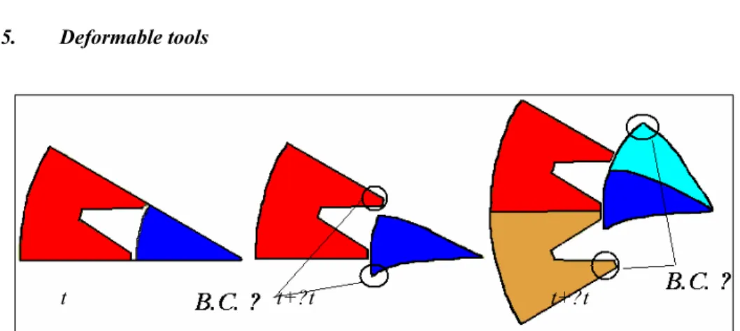
3.5. Deformable tools

Figure 6. Periodicity conditions for problems with deformable tools. One portion of

tool and workpiece at time t. Loss of correspondence at time t+∆t. Same loss of correspondence at time t+∆t with two portions of each.

One of the objectives of the finite element simulation of gear forging is to produce net-shape parts, so the coupled elastic deformation of the dies must be considered, following the method presented in (Barboza et al. 02, Pichelin et al. 01). For helical gears, it is important to take into account the recurrent boundary conditions [40] and [42], both for the workpiece and for the dies. However, because a Lagrangian approach is been used, the symmetry surfaces SA and SB are not steady (see figure 6) and their deformations follow the ones of the material flow. When using rigid dies, it is often necessary to discretize more than one tooth of the die in order to impose the proper boundary conditions, because very often the workpiece material flows into more than one tooth of the tool (see figures 6, 13, 16, 17). When using deformable dies, these deformations are not the same for the workpiece and for the dies (see last two examples of section 4). Therefore, it is virtually impossible to carry out the

simulation with only one tooth. Adding another “tooth” for the tool (yellow in figure 6) and for the workpiece (light blue in figure 6) does not help. In fact, there is still a region of the workpiece and a region of the tool without any boundary conditions (see figure 6). It order to avoid this, which would prevent us from using the recurrent boundary conditions with deformable tools, more tricky boundary conditions must be introduced.

3.6. Algorithm for deformable tools

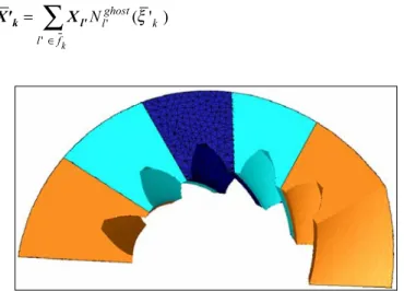
The surface ∂Ωtool of the deformable tool is regarded as the master surface for the contact algorithm with the workpiece (see section 2). In order to make it possible to also detect the contact in a “void” area, in which it is not desired to actually compute the tool deformation, the surface of the tool is first duplicated and then rotated by the

R rotation. So, it produces a “ghost” surface ∂Ωghost (see figure 7) in this “void” area. During this rotation, the correspondence of nodes between the initial and rotated tools is saved for the contact analysis. This construction of “ghost” surfaces can be repeated as many times as necessary, for instance, if the material is expected to flow into more than 3 teeth of the tools. Figure 7 shows only one “ghost” surface, while figure 8 provides a 3D example with two “ghost” surfaces on each side.

Figure 7. Deformable tools. Creation of a “ghost” surface ∂Ωghost of the tool. Section view of a meridian plane of the symmetry axis.

Let us consider a node k of the workpiece surface that is in contact with ∂Ωghost and denote by X ' the orthogonal projection of X_k k onto it: ' ( k)

ghost

k X

X =π . Let us also

∑

∈ = k f l k ghost l N ' ' (ξ' ) l' k X ' X [46]

Figure 8. Initial surface mesh (in the centre) and ghost meshes for the contact

analysis: two “ghosts” on each side of the initial mesh.

According to the construction process of ∂Ωghost, there is a facet f of the original k tool surface mesh that corresponds to f , such that:k

s.t. k k l ' l l' f , l f , X R X ∀ ∈ ∃ ∈ = ⋅ and k t ghost k k l l ' k l f X R X ' X N ( ' )ξ ∈ = =

∑

[47] Therefore:

∑

∑

∈ ∈ = ⎟ ⎟ ⎠ ⎞ ⎜ ⎜ ⎝ ⎛ ⋅ = ⋅ = k k l f k ghost l l k f l k ghost l T X TN N_' (ξ' ) , ( ' ) _' (ξ' ) l k k ) R V(X ) R V ' X V( [48]

So, the contact boundary conditions for the “void” regions become:

(

)

, 0 _k ( '_k) k X T T t ≤ = ∆ − ⋅ − k δ k k V(X' ) n V [49]

4. APPLICATIONS

4.1. Academic test: evaluation of accuracy and time reduction

A test series has been conducted to validate the method. It consists in running the same simulation with plane and recurrent symmetries. One test is quite academic while the other is derived from an actual process.

The accuracy of the penalty method, which is utilised to enforce the recurrent boundary conditions for the mechanical and thermal problems, is first evaluated. A simple benchmark test consists in forging a quarter of a cylinder between two rigid dies (see figure 9). The meshes of the symmetry surfaces are coincident, with 80 nodes, so that the recurrent conditions can be perfectly imposed.

Figure 9. Upseting of a cylinder with recurrent boundary conditions. Initial and

final configurations. Isovalues of equivalent total deformation at the end.

Firstly, it can be noticed that the deformation field is identical on the both master and slave surfaces (see figure 9), which shows a proper handling of the symmetry conditions. Both for the mechanical and the thermal problems, the relative and maximal errors are considered to quantify the difference between the velocities and

(

V RV(X )

)

) X RV( V k k k k ~ max and ~ _ _ = − − = ∈ ∈ ∈

∑

∑

B B B S k max mech S k k S k rel mech err V err [50] MECHANICAL THERMAL sym ρ ther ρ Nb of iterations for resolution rel mech

err _{_} err_{mech_max}

[mm/s] Nb of iterations for resolution rel therm

err _{_} err_{therm_max}

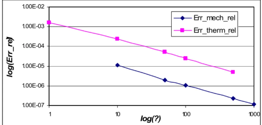
[0C] 1 32 1.6*10-3 6.23 10 700 1.1*10-5 4.0*10-4 55 2.4*10-4 0.81 50 1000 2.0*10-6 8.0*10-5 104 5.0*10-5 0.16 100 1500 1.1*10-6 4.2*10-5 123 2.5*10-5 0.08 500 2600 2.3*10-7 8.5*10-6 168 5*10-6 4.2*10-5 1000 3100 1.2*10-7 4.2*10-6

Table 1. Accuracy of the penalty methods according to the penalty coefficient.

1.00E-07 1.00E-06 1.00E-05 1.00E-04 1.00E-03 1.00E-02 1 10 _log(?) 100 1000 log(Err_rel ) Err_mech_rel Err_therm_rel

Figure 10. Error versus the value of the penalty coefficient in logarithmic scale.

In this particular case with coincident meshes, _δk =0

so the k _∆t

/

δ term does

not appear in equations [50]. The errors are written in a similar way for the thermal problem.

Figure 10 shows that there is a linear dependency between the penalty coefficients and the mechanical and thermal errors, which is quite typical for a penalty method. On the other hand, table 1 shows that the CPU time (number of system resolutions) is increased by a factor of 2 when the errors are decreased by a factor of 10. Practically, penalty coefficients of 100 are used, both for mechanical and thermal problems, so providing accuracies that are consistent with the ones of the contact algorithm.

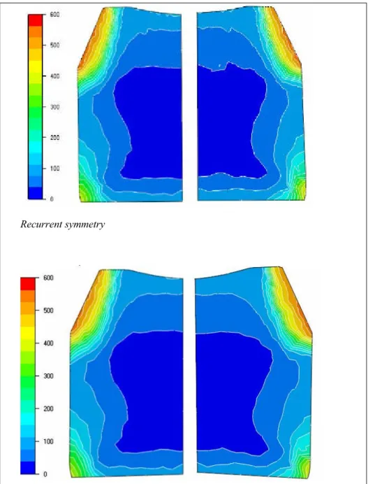
A second test consists in forging one tooth of an actual conical straight gear. The workpiece has a complex elasto-viscoplastic behaviour, and the tools have realistic geometries (see figure 11). This simulation is carried out both using plane symmetries and recurrent boundary conditions. In figure 11, the geometries are obtained with plane symmetries. The qualitative comparisons of figure 12 are made after few increments, just before the first remeshing, in order to make it possible to compare the values at exactly the same coordinates, and to avoid the noise caused by remeshing. The obtained results are almost identical with both approaches. For example, the values of the equivalent stress (see figure 12) and of the forging effort differ by less than 10-4 in relative values.

Recurrent symmetry

Plane symmetry

Figure 12. Equivalent stress on symmetry surfaces after 3 % of forging with plane

However, the CPU time is multiplied by a factor of 2 with recurrent conditions. This is due to the fact that the flow is less constrained while the coupling between the opposite sides of the domain is very severe. It results into a worsening of the conditioning of the linear system, and consequently into an increase of the computational time. This phenomenon is noticed in all numerical tests, independently on the complexity of the geometries or material behaviours. So, also taking into account that the computational complexity of the solver is proportional to

Ndof3/2, it is possible to evaluate the CPU time reduction provided by recurrent symmetries. For a helical gear with 10 teeth, the recurrent boundary conditions allow reducing the computational time by an estimated factor of 15.

4.2. Industrial test: helical gear forging:

The actual forging of a 16 teeth helical gear is considered (see figure 13), where the workpiece is free to rotate around its axis during the process. Consequently several teeth of the rigid matrix have to be considered for proper handling of the contact surface. The material is modelled by an elasto-viscoplastic constitutive equation.

Figures 14.a, 14.b and 14.c show that the velocity, temperature and deformation fields are almost identical on the master and the slave surfaces. So the velocity and temperature boundary conditions can be regarded as properly imposed, and the master/slave approach as quite accurate. At the end of the process, the gap between the corresponding symmetry faces provides an overall measure of the cumulated errors. It is less then 10-4in relative values (with respect to the mesh size) (see figure 14.d), which is consistent with the accuracy of the contact formulation. By duplicating and rotating the obtained final part, figure 15 shows that the corresponding surfaces match properly and that they have actually been subjected to the same deformations.

It is noticed that the workpiece rotates around the symmetry axis during forging, as it is the case in the actual process. In this case, the computational time reduction provided by this approach is estimated around 30.

a) Z Velocity b) Temperature

c) Deformation d) Contact on the slave surface Figure 14. Isovalues on the master and slave surfaces.

Figure 15. Final configuration: fully reproduced and only with 5 teeth of the

workpiece, while the simulation was carried out only on 1 tooth (mesh of left figure).

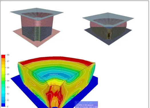
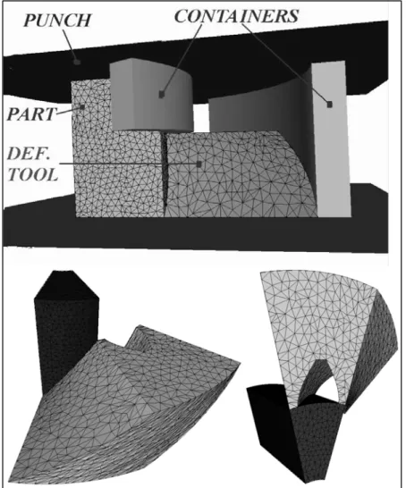
4.3. Gear forging with deformable dies

In order to evaluate the accuracy and the robustness of the proposed approach with deformable tools, an academic gear-like forging process is proposed in figure 16. A viscoplastic constitutive law (with a linear behaviour, mpart=mtool=1) is used for the two bodies, workpiece and tool, in order to trigger complex velocity fields both on the symmetry surfaces and on the contact surfaces. However, the consistency K of the tool material is 10 times larger than the workpiece one: Kpart=20MPa, Ktool=200MPa.

As it can be seen in figure 16, “ghosts” surfaces are necessary from the beginning of the simulation, because the symmetry surfaces are not the same for the workpiece and for the tool. This particular case, which corresponds to a more friendly way to set up simulation data, can only be handled with the proposed method. In figure 17, it is very clear that the workpiece is in contact with the tool, both with its actual and ghost descriptions.

Figures 18 and 19 show that the recurrent symmetry conditions are accurately satisfied at the end of the calculations. Figures 18 shows that the contact conditions between the deformable bodies are properly imposed, even in the “ghost” zones. Both for the workpiece and for the deformable die, the gaps between the master and slave symmetry surfaces are very small, and can be regarded as negligible, as in previous example.

Figure 16. Helical gear forging with deformable dies. Different views of the initial

Figure 18. Forging of a helical gear with deformable dies: deformed tool and

workpiece at the end of the process, after reconstruction of 3 teeth.

Figure 19. Forging of a helical gear with deformable dies: workpiece deformation

5. CONCLUSIONS

Recurrent boundary conditions are an efficient way to reduce the CPU time for helical gear simulation. The proposed implementation can be regarded like an extension of the bilateral contact algorithm between deformable surfaces. The utilised master / slave approach is both stable and accurate. It does not require coincident meshes or more complex formulations like Arbitrary Eulerian Lagrangian ones. The use of «ghost» surfaces makes it possible to extend it to multi-bodies problems, as encountered in the forging with deformable dies.

In some particular cases, this approach may suffer from some of the usual limitations of the master / slave method, if it happens that the symmetry surfaces exhibit very different mesh refinements. In these cases, it is possible that no recurrent boundary condition is imposed to some nodes of the master surface, which would provide locally wrong solutions. In order to avoid this, a more accurate contact formulations should be used, like the quasi-symmetric approach proposed in (Fourment et al. 04) or similar approaches.

ACKNOWLEDGEMENTS

The authors gratefully acknowledge support from the French government and the companies involved in the Simulforge project managed by CETIM, and more particularly the Ascoforge company for providing the validation cases.

REFERENCES

Aliaga C., Massoni E., 3D numerical simulation of thermo-elasto-visco-plastic behaviour

using stabilized mixed finite element formulation: application to heat treatment,

Proceedings of the Sixth International Conference on Numerical Methods in Industrial Forming Processes, Huetink, J.; Baaijens, F.P.T. (editors), A.A. Balkema, Rotterdam, Netherlands, pp 263-269, 1998

Barboza J., Fourment L. and Chenot J.-L., Contact algorithm for 3D multi-bodies problems:

application to forming of multi-material parts and tool deflection. In WCCM V - Fifth

Congress on Computational Mechanics. 2002. Wien, Austria

Bathe K.J. and Abbasi N.E., On a new Segment to Segment Contact Algorithm, in Computational Fluid and Solid mechanics, K.J Bathe, Editor. 2001, Elsevier Science Coupez T., A mesh improvement method for 3d automatic remeshing, Numerical Grid

Generation in Computational Fluid Dynamics and Related Fields, pp 615-626, Weatherill,N.P. (editor), Pineridge Press, 1994

Fourment L., Popa S. and Barboza J., A Quasi-symmetric Contact Formulation For 3D

Problems. Application To Prediction Of Tool Deformation In Forging, The 8th

Conference On Numerical Methods in Industrial Forming Processes, Columbus, Ohio, USA, June 2004

Huang G., Gear Forging Simulation Using Cyclic Symmetry, Proceedings of the Heigth International Conference on Numerical Methods in Industrial Forming Processes, Ghosh S., Castro J.M., Lee J.K. (editors), Springer-Verlag, New York, 1998

Park Y.B. and Yang D.Y., Finite element analysis for precision cold forging of helical gear

using recurrent boundary conditions, Proc Instn Mech Engrs Vil 2/2 Part B, 7 October

1997

Pichelin E., Mocelin K., Fourment L. and Chenot J.-L., An application of a master slave

algorithm for solving 3D contact problems between deformable bodies in forming processes, Revue Européenne des Eléments Finis, 10-8, 85, 2001

BODIES

FOR LARGE 3D DEFORMATIONS SOLID

MECHANICS

L. Fourment

*

, S. Popa

CEMEF, Ecole des Mines de Paris, B.P. 207, 06 904 Sophia Antipolis Cedex, France

Abstract

A quasi-symmetric formulation is proposed for contact between deformable bodies to avoid the shortcomings of standard master / slave approaches when the master body is more finely meshed than the slave body. It uses a double pass algorithm for symmetric contact detection and a projection of slave body contact pressures onto the master surface. This method applies either to integral or nodal contact formulations, the latter being used for applications. It is compared to the standard formulation for different numerical tests and on complex 3D forging applications.

Keywords: Finite elements, Contact, Non matching meshes, Large deformations

1. INTRODUCTION

This paper investigates a quasi-symmetric formulation for contact between deformable bodies, which has been developed to avoid the usual shortcomings of standard master / slave formulations without too many complications. It is well known that when the meshes of the contact interfaces do not match after finite element discretization, which is the most general case, the contact conditions cannot be handled symmetrically. The symmetric two-pass algorithms, where the contact conditions between body A and body B are super-imposed to the conditions between body B and A, produce over-constraint formulations with numerical locking of the contact interface [1-3]. In the standard master / slave approach, only the selected slave body is prevented from penetrating the master body. It so avoids locking. This approach is quite satisfactory when the bodies have meshes of consistent refinements on the contact interface. When they are matching, the formulation is perfectly symmetric. On the other hand, when the mesh of the master body is much finely refined than the mesh of the slave body, the formulation loses its symmetry, so the non-penetration condition is not properly imposed for the master surface. Consequently, it may occur that parts of this surface are numerically regarded as being free, which may allows significant and unacceptable penetrations. From a numerical point of view, the convergence rate of the finite element method is not only lower in this case, but the accuracy of the solution decreases when the number of the master nodes increases. This standard approach paradoxically provides worse and worse solutions when the master body is more finely refined.

*

Corresponding author. Tel. : +33 4 93 95 75 95 ; fax : +33 4 92 38 97 52 E-mail address: lionel.fourment@ensmp.fr