858 THE LEADING EDGE October 2017
G
e o p h y s i c a lT
u T o r i a l— c
o o r d i n a T e d b yM
a T Th
a l lColored inversion
W
hether it is deterministic, band-limited, or stochastic, seismic inversion can bear many names depending on the algorithm used to produce it. Broadly, inversion converts reflectivity data to physical properties of the earth, such as acoustic impedance (AI), the product of seismic velocity and bulk density. This is crucial because, while reflectivity informs us about boundaries, impedance can be converted to useful earth properties such as porosity and fluid content via known petrophysical relationships.Lancaster and Whitcombe (2000) published a fast method for band-limited inversion of seismic data known as colored inversion (CI) that generated widespread interest among inter-preters. Recognizing that the popular sparse-spike inversion process could be approximated by a single operator, yielding relative impedance via simple convolution with the reflectivity data, the authors showed that this operator can be derived from well logs. Like other inversions, CI can help remove the smearing effects of the seismic wavelet and enhance features such as thin beds and discontinuities. What’s more, since CI is directly linked to seismic data, the relative impedance it produces can be used as a base for comparison with other inversion to see what kind of information is introduced by numerical constraints or the low-frequency model.
In this tutorial, we follow the steps presented by Lancaster and Whitcombe in their 2000 expanded abstract to achieve the so-called “fast-track colored inversion.” Using open-source algo-rithms, we describe all the steps to go from reflectivity data to inverted cubes:
1) Fit a function to the log spectrum(s).
2) Get a difference spectrum by substracting the seismic spectrum.
3) Convert the difference spectrum to an operator.
4) Convolve the operator with the stacked seismic.
5) As a quality control (QC) step, check the residuals by comparing log and AI section spectrums. The idea of this tutorial is to achieve a CI without any external software, just Python code with the NumPy and SciPy libraries. You can read and run the code for yourself from the repository at github.com/seg/tutorials-2017. This tutorial focuses on presenting the whole workflow in the simplest fashion rather than trying to optimize parameters to recover interpretable features. Prior to
Martin Blouin
1and Erwan Gloaguen
2running the workflow on your data, noise attenuation should be performed to ensure that the inversion process recovers frequencies associated only with the earth.
The data set
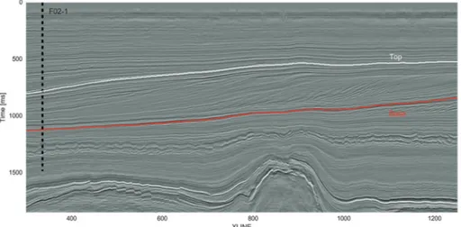
For our demonstration, we use one inline from the 1987 Dutch F3 volume (Figure 1) plus the AI log from the F02-1 well. Good descriptions of the geologic setting of this data set can be found in Sorensen et al. (1997) and Overeem et al. (2001). We use the dip-steered median filter stacked data set to get reduced noise on our input.
Fit a function to the log spectrum
Walden and Hosken (1985) observed that the reflectivity sequences in sedimentary basins display a logarithmic decay in amplitude as frequency increases. For the first step of our inversion, we look at the reflectivity spectrum and make sure it behaves as predicted. We load the F02-1 well, convert it to the time domain, and calculate the spectrum (Figure 2).
n_log = AI_f021.shape[0] k_log = np.arange(n_log-1)
Fs_log = 1 / np.diff(time_f021/1000) T_log = n_log / Fs_log
freq_log = k_log / T_log
freq_log = freq_log[range(n_log//2)] spec_log = np.fft.fft(AI_f021) / n_log spec_log = spec_log[range(n_log//2)]
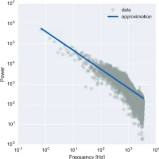
We would like to simplify the spectrum, so we proceed to a regression. To make the process more robust, CI packages offer
1GeoLEARN Solutions.
2INRS-ETE. https://doi.org/10.1190/tle36100858.1.
Figure 1. F3 dip-steered median filtered stacked seismic data at inline 362 with well location and bounding
horizons of the inverted region.
October 2017 THE LEADING EDGE 859 one for the error function. We then use scipy.optimize to find the best fit, shown in Figure 3.
def linearize(p, x): return p[0] * x**p[1]
def error(p, x, y):
return np.log10(y) - np.log10(linearize(p, x)) args = (freq_log[1:2000], np.abs(spec_log[1:2000])) qout, success = optimize.leastsq(error,
(1e5, -0.8), args=args, maxfev=3000)
Compute the difference
Now we have a continuous function that mathematically approximates the well-log spectrum. The next major step of the workflow is to compute an operator that is representative of the difference between the log spectrum and the seismic spectrum.
We first define some boundaries to our modeled spectrum in the frequency domain. This is a critical part that will have great influence on the end result. We define a simple function to generate a 50-points Hanning-shaped taper at both ends of the spectrum; the result is shown in Figure 4. Then we take seismic traces at the well location, average them, and repeat the procedure we did on the well to get the spectrum. Figure 4 shows the resulting modeled spectrum. In this example, taper windows of 0–5 Hz and 100–120 Hz have been defined. It is important to note that our end result will be influenced greatly by this choice, and care should be applied at this stage.
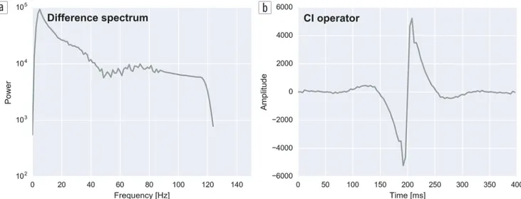
After this step is completed, we simply substract the seismic spectrum from our modeled spectrum (Figure 5).
Convert to an operator
Now, continuing with Lancaster and Whitcombe’s methodol-ogy, we can derive an inversion operator. We move back to the time domain with an inverse Fourier transform, then shift zero time to the center of the time window. Finally, we rotate the phase by taking the quadrature of the signal, represented by the imagi-nary component and shown in Figure 5.
gap = spec_log_model - spec_seismic_model operator = np.fft.ifft(gap)
operator = np.fft.fftshift(operator) operator = operator.imag
Convolve operator with seismic
Once the operator is calculated a simple trace-by-trace convolu-tion with the reflectivity data is needed to perform CI. NumPy’s apply_along_axis() applies any function to all columns of an array, so we can pass it the convolution:
def convolve(t):
return np.convolve(t, operator, mode='same') ci = np.apply_along_axis(convolve, axis=0, arr=seis)
Figure 2. F02-1 well data. (a) AI log and (b) calculated power spectrum.
Figure 3. F02-1 well spectrum approximated by a linear function in log space.
Figure 4. Comparison of well log, seismic, and modeled frequency power spectrum.
you the option of averaging this spectrum over all the available wells, but we can skip that as we are working with only a single well. To proceed to a linear regression, we define two simple functions, one that serves as the linearization of the problem and
860 THE LEADING EDGE October 2017
Since the relative impedance result contains no low frequencies, it does not inform us about trends, so it makes more sense to look at the result in a single formation. We will focus on an area of interest of about 300 ms in thickness between two horizons; Figure 6 presents the resulting relative impedance section scaled (0–1) in this area.
Check the residuals
To make sure we did a good job defining our operator, we now look at the spectrum from the relative impedance result at the well location to see if we achieved a good fit with the well-log spectrum (Figure 7). It is to be noted that this fit was achieved with some arbitrary decisions, and the workflow could be iterated upon to try to minimize the difference between the two spectrums.
Conclusion
We have presented a straightforward application of CI using only Python with the NumPy and SciPy libraries. This open-source workflow is documented at github.com/seg. It is called a “robust” process in the literature, but it is somewhat sensitive to the chosen frequency range. There are also choices to be made about the window of application and the number of traces used to compute the seismic spectrum. Notwithstanding all this, the process is simple and fast and yields informative images to interpreters.
Acknowledgment
Thanks to Matt Hall for useful comments and suggestions on the workflow and manuscript.
Figure 5. (a) Resulting difference spectrum. (b) Associated operator.
Figure 6. Relative impedance result in a single stratigraphic unit.
Figure 7. QC of the CI workflow by comparison between input and output spectrums.
October 2017 THE LEADING EDGE 861 Corresponding author: martin.blouin@geolearn.ca
References
Lancaster, S., and D. Whitcombe, 2000, Fast-track ‘coloured’
inver-sion: 70th Annual International Meeting, SEG, Expanded
Abstracts, 1572–1575, https://doi.org/10.1190/1.1815711. Overeem, I, G. J. Weltje, C. Bishop-Kay, and S. B. Kroonenberg,
2001, The Late Cenozoic Eridanos delta system in the Southern North Sea Basin: A climate signal in sediment supply?: Basin Research, 13, no. 3, 293–312, https://doi.org/10.1046/j.1365-2117. 2001.00151.x.
Sørensen, J. C., U. Gregersen, M. Breiner and O. Michelsen, 1997, High frequency sequence stratigraphy of upper Cenozoic deposits: Marine and Petroleum Geology, 14, no. 2, 99–123, https://doi. org/10.1016/S0264-8172(96)00052-9.
Walden, A. T., and J. W. J. Hosken, 1985, An investigation of the spectral properties of primary reflection coefficients: Geophysical Prospecting,
33, no. 3, 400–435, https://doi.org/10.1111/j.1365-2478.1985.
tb00443.x.
Suggestions for further reading
dGB Earth Sciences and TNO, 1987, F3 data set. Data set accessed 31 August 2017 at http://opendtect.org/osr/.
Francis, A., 2014, A simple guide to seismic inversion: GEOExPro,
10, no. 2, 46–50.
© The Author(s). Published by the Society of Exploration Geophysicists. All article content, except where otherwise noted (including republished material), is licensed under a Creative Commons Attribution 3.0 Unported License (CC BY-SA). See https://creativecommons.org/licenses/by-sa/3.0/. Distribution or reproduc-tion of this work in whole or in part commercially or noncommercially requires full attribution of the original publication, including its digital object identifier (DOI). Derivatives of this work must carry the same license.