Faculté des
lettres
et
sciences humaines
Département de géomatique appliquée
Université de
Sherbrooke
Characterisation of night-time aérosols using
starphotometry
Konstantin Baibakov
Mémoire présenté pour l'obtention du grade de Maître en sciences
géographiques
(M.
Se.), cheminement télédétection
Juillet 2009
Abstract
This is a
study concerning the use of starphotometry to retrieve night-time aérosol optical
depths (AODs). In the summer of 2007 a SPSTAR03
starphotometer was installed at a
rural site at Egbert, Ontario for the purpose of the nighttime AOD measurements. Twosériés of daytime / nighttime AODs were acquired using the CIMEL CE 318
sunpho-tometer and the SPSTAR03 from Aug. 31 to Sept. 19 2007 and from June 30 to July 5,
2008. The measurements were complemented by vertical backscatter coefficient profiles acquired using a pulsed lidar. We found that starphotometer AOD estimâtes, based on
the application of a two star method
(TSM)
to low and high élévation stars, are suscepti
ble to atmospheric inhomogeneity effects. Starphotometer AOD estimâtes based on the one star method (OSM) reduce this sensitivity but require absolute calibration values.
A level of continuity was obtained between the daytime sunphotometry and nighttime
starphotometry data. A continuity parameter (defined as the average différence between
the measured nighttime and interpolated daytime values) was calculated over four dis
tinct periods. It yielded the différences of 0.160, 0.053, 0.139 (total, fine and coarse mode
optical depths) for the low star and 0.195, 0.070, 0.149 for the high star. We
argue that
cloud screening would have reduced the continuity parameter différences for the coarse and total optical depths. For 5 ont of 8 nights of lidar opération, a combination of the
Angstrom and Spectral Deconvolution Algorithm (SDA)
analysis provided an indication
of the nature of the atmospheric features seen in the lidar data. Fine and coarse-mode
events were detected during the measurement periods using the SDA. Lidar data was
used to better understand complex atmospheric phenomena and was found especially
effective for cloud détection and général signal increase/decrease analysis.
Keywords: starphotometry, aérosols, aérosol optical depth, Egbert, sunphotometry, lidar.
Résumé
Caractérisation des aérosols de nuit par photométrie stellaire
C'est une étude sur l'utilisation de la photométrie stellaire afin d'obtenir l'épaisseur
optique des aérosols (AOD)
durant les périodes nocturnes. Au cours de l'été 2007, le
photomètre stellaire SPSTAR03 était installé sur un site rural d'Egbert, Ontario pour
prendre des mesures nocturnes de l'AOD. Deux séries de mesures diurnes/nocturnes de
l'AOD ont été effectuées avec le photomètre solaire CIMEL CE-318 et SPSTAR03 entre le31 août et le 19 septembre 2007 et entre le 30
juin et le 5
juillet 2008. Ces mesures étaient
accompagnées par les profils verticaux du coefficient de rétrodiffusion acquis avec un
li-dar à pulsation. Nous avons trouvé que les AODs
estimées par le photomètre stellaire en
appliquant la méthode de deux étoiles (TSM)
aux étoiles d'élévation basse et haute, sont
sensibles aux inhomogénéités atmosphériques. Les estimations d'AOD basées sur une
méthode d'une étoile (OSM)
réduisent cette sensibilité mais en même temps nécessitent
les valeurs de calibration absolues. Une certaine continuité a été obtenue entre la pho
tométrie solaire de jour et la photométrie stellaire de nuit. Un paramètre de continuité
(défini comme
la différence moyenne entre les valeurs mesurées de nuit et les valeurs inter
polées de jour) était calculé sur quatre périodes différentes. Les différences étaient 0.160,
0.053, 0.139 (l'épaisseur optique total, l'épaisseur optique des modes fin et large) pour
l'étoile basse et 0.195, 0.070, 0.149 pour l'étoile haute. Nous affirmons qu'un algorithmede filtrage des nuages réduirait les différences du paramètre de continuité pour l'épaisseur
optique totale ainsi que celle dans le mode grossier. Pour 5 des 8 nuits d'opération du
lidar, la combinaison de l'analyse d'Angstrom et de l'Algorithme Spectral de
Deconvo-lution (SDA)
a apporté une indication sur la nature des caractéristiques atmosphériques
vue dans les données lidar. Les événements des modes fin et large étaient détectés avec
le SDA durant ces périodes de mesures. Les données lidar étaient utilisées afin de mieux
comprendre les phénomènes atmosphériques. Elles étaient particulièrement efficaces dans
la détection des nuages et dans l'analyse des tendances générales d'augmentation et de
diminution du signal.
Mots clés: photométrie stellaire, aérosols, épaisseur optique des aérosols, Egbert,
Acknowledgments
Foremost, I would like to thank my thesis director, Prof. Norm O'Neill, who is net only
a great scientist, but also a caring and supportive advisor, who bas provided me with
some unique opportunities to learn and grow.
I would like to thank Chris Green and Pranke Fronde of the Center for Atmospheric
Research Experiments (GARE)
at Egbert for their logistics support in regard to the
installation and use of the starphotometer.
Fm grateful to Bernard Firanski who bas not only acquired most of the starphotom-etry data used in this work, but also taught me many things about lidars.
ALIAS lidar data was kindly provided by Kevin Strawbridge and Bernard Firanski of Environment Canada. Sunphotometry data was obtained from the AERONET website for Egbert, for which the principal investigator is Norm O'Neill.
My sincere thanks go to Dr. Lucas Alados who bas kindly agreed to be an external reviewer for this thesis.
It is with great pleasure that I acknowledge ail the friends and collègues who made
my Sherbrooke experience a truly enriching one.
My most profound gratitude goes to my family and especially to my parents for their
unconditional love and support. Without them nothing would be possible.
This Project was financially supported by the Natural Sciences and Engineering Re
search Gouncil of Canada
(NSERC),
Canadian Foundation for Climate and Atmospheric
Sciences (CFCAS),
Le Fonds Québécois de la Recherche sur la Nature et les Technologies
Contents
List of Figures : . . . iv
List of Tables v
1 Introduction 1
1.1 Atmospheric aérosols, their variability and sources 1 1.2 The importance of aérosols in climate forcing 2
1.3 Aérosol optical depth 2
1.4 Nighttirne AOD variability - the focus of the présent work 3
2 Hypothesis, project objectives and research site 5
2.1 Hypothesis 5
2.2 Project objectives 5
2.2.1 Acquisition of a first représentative AOD time sériés with
SP-STAR03 in Canada 5
2.2.2 Optical and physical cohérence analysis of SPSTAR03 measurements 6
2.3 Research site (Egbert, Ontario)
6
3 Methodology 9
3.1 Methodological Flow Chart ■ 9
3.2 Theoretical background ; . . . 9
3.2.1 Total optical depth 9
3.2.1.1
Rayleigh optical depth, ÔRay
12
3.2.1.2 Ozone optical depth, Sozme 12
3.2.1.3 Water vapor optical depth, SH2O 13
3.2.1.4 Nitrogen dioxide optical depth, 14
3.2.2 Aérosol optical depth, AOD 15
3.2.3 Angstrom Exponent 15
3.2.4 Spectral Deconvolution Algorithm ■. . 16
3.3 Measurement methods and instruments 17
3.3.1 Sunphotometry 17
3.3.1.1 CIMEL CEl-318 Sunphotometer 18
3.3.2 Starphotometry 19
3.3.2.2 One-star method 22
3.3.2.3 Sensitivity of the Twostar method 23
3.3.2.4 SPSTAR03 starphotometer 25
3.3.2.5 Measurement stars and TSM limitations 28
3.3.3 Lidar Measurements 29
■3.3.3.1 Lidar équation 30
3.3.3.2 AOD estimâtes from the lidar profile 31
3.3.3.3 ALIAS 32
4 Principal results obtained 34
4.1 Summary of the data obtained 34
4.2 Starphotometry and night-time lidax data 34
4.2.1 TSM results 35
4.2.2 Calibration periods for the OSM ' 35
4.2.3 OSM results 36
4.2.4 Angstrom exponent analysis and SDA 37
4.2.5 Lidar data 37
4.2.6 Sunphotometry data and continuity analysis 38
5 Discussion of the results, recommendations and future work 42
5.1 SPSTAR03 operational issues and considérations 42
5.2 TSM and OSM measurements 43
5.2.1 Stability of the OSM calibration values 43
5.2.2 TSM and OSM data 44
5.2.3 Angstrom analysis and SDA, corrélation -with lidar data 46
5.2.4 Continuity analysis 64
5.2.5 Recommendations and future -work 65
5.2.6 Arctic installation .' 66
6 Conclusions 68
A A list of Bright Stars 71
B Extra-terrestrial intensities 74
List of Figures
2.1 SPSTAROS's location at CARE 8
3.1 Methodological flowchart 10
3.2 Typical SPSTAR03 spectrum 14
3.3 Sunphotometry principle 18
3.4 CIMEL CE-318 19
3.5 Two-star inethod 21
3.6 One-star method 23
3.7 Modelled TSM perturbations (high star)
24
3.8 Modelled TSM perturbations (low star)
. 25
3.9 Principal components of SPSTAR03 starphotometer 26
3.10 SPSTAR03 schematical diagram 27
3.11 Lidar operating principle 29
4.1 OSM calibration periods 36
4.2 Measurements summary 38
4.3 Continuity analysis 40
5.1 Time sériés of Moi for 7001
(Vega)
44
5.2 Measurement AOD spectra 45
5.3 Combined data sets for selected dates 48
5.4 Starphotometer in the Arctic
^
66
B.l Extra-terrestrial intensities of selected stars 75
List of
Tables
3.1 Spectral O3 absorption coefficients 13
4.1 Measurements summary 34
4.2 Conventional star names 35
4.3 Continuity parameter values 39
Chapter 1
Introduction
Radiative energy balance is among the essential attributes of the Earth's climate. It is defined as the balance between incoming shortwave solar radiation which is reflected and
absorbed by the atmosphère and the earth's surface and reemitted as infrared (longwave)
radiation. This fine balance can be perturbed by even small changes in atmospheric
properties, such as aérosol loading, variable cloud cover and abundances of greenhouse
gases. Among ail the influences on the radiative balance, aérosol effects are associated
with the largest uncertainty {IPCC, 2007). Having a better compréhension of aérosol
phenomena (like their formation, transport and interaction mechanisms), will directly
resuit in more accurate climate models and hence an improved capacity to predict climate change.
1.1 Atmospheric aérosols, their variability and sources
Aérosols are small particles suspended in the atmosphère whose size ranges from « 0.01
to lOO^im {Hinds, 1999). They exhibit a multitude of shapes, sizes and chemical compo
sitions and are highly variable in time and space. This large variability can, in part, be
attributed to the variety of aérosol forming processes. Biomass burning fîres, wind-blown
deserts, volcanic éruptions and océan wave processess are some of the major natural
aérosol sources. Human activities can also resuit in the production of aérosols, with the
1.2 The importance of aérosols in climate forcing
Aside from better known effects such as the influence on human health or decreased
visibility in polluted areas, aérosols are associated with climate change phenomena whose influence can be separated into direct and indirect eflFects. The direct effect refers to the backscattering and absorption of solar energy by aérosols during its propagation through
the atmosphère. The former (more dominant effect) results in the cooling of the ground
and the troposphère while the latter can (in the case of strongly absorbing aérosols) warm
the atmosphère. The indirect aérosol effect is due to the presence of the aérosols within or near clouds. Aérosols acting as cloud condenstation nuclei can significantly alter
the physical and optical properties of clouds and consequently their radiative impact. Aérosols accordingly have an important influence on atmospheric radiative properties and thus on the radiative energy budget. Indeed their predominantly cooling effect can be viewed as a mitigating factor opposing the generally climate warming influence of the atmosphère. A comprehensive and detailed overview of the aérosols' rôle in the climate
processes can be found in IPCC,
2007
(ch. 2.4).
1.3 Aérosol optical depth
Aérosol optical depth (AOD) is a fondamental parameter for characterizing the optical
effets of aérosols . It represents the extinction (absorption and outscattering) losses due
to aérosols over a certain path in the atmosphère (the standard définition being the total
aérosol optical depth in the vertical direction). Furthermore, the spectral (wavelength)
dependency of the AOD provides information on average aérosol size. There currently exist two principal approaches for estimating AOD values: through ground-based and satellite measurements. The later approach can provide global aérosol coverage but is
lim-ited in scope and accuracy {Dubovik et ai, 2002), and requires ground-based validation.
On the other hand, ground-based AOD estimations, while being much more spatially sparse, are presently best suited for the analysis of aérosol optical properties because of their higher accuracy, temporal resolution and temporal extent. During the day, AOD
is traditionally measured with a ground-based sunphotometry, a technique that makes
use of the atténuation of the solar radiation propagating through the atmosphère {Shaw,
1983). Sunphotometers are used around the world and are usually grouped in networks
NETwork, Holben et a/., 1998) is the largest and most globally dispersed sunphotometer
network.
1.4 Nighttime AOD
variability -
the focus of
the présent
work
A
complété analysis of the spatial and temporal distribution of aérosol optical properties
nécessitâtes continuons observations during the day and night. For example, using only the sunphotometry one can potentially be missing a significant portion of measurements in the 24-hour cycle. The problem is evén more aggravated at the Earth's pôles, where a night lasts several months. Furthermore, night-time periods présent a spécial interest
because of their distinctive radiative, chemical and meteorological phenomena associated
with a lack of sunlight. Some examples of the day-night différences in aérosol effects
can be found in Jacobson, 1998 (effects of urban aérosols on photolysis rate coefficients
and température profiles) and Legrand et al, 1988 (effects of dust layers on the ground
température).
While there has been substantial progress in the methodological and instrumental
aspects of aérosol measurements in général, traditional ground-based and satellite AOD measurements are largely limited to the daytime. Lidar instruments are mostly used for providing vertically resolved aérosol profiles but can also give a measure of AOD during the night. The accuracy of lidar retrievals, however, typically dépends on a specified
ratio between the aérosol extinction and backscatter coefficients {Cattrall et al, 2005).
This altitude-dependent ratio can not, in the absence of complementary (and logistically
difficult) measurements, be precisely determined as it is varies significantly depending on
the aérosol type (idem). Some aérosol information can also be retrieved with ceilometers
despite their primary use being the détermination of the cloud heights {Mûnkel et ai,
2007). Ceilometers are optically simpler, commercially available low-power lidars with
temporal and vertical resolutions lower than with the more expensive and challenging to maintain research-grade lidars. Reported aérosol concentrations are typically of the
order-of-magnitude nature with only the lower troposphère taken into account {Zéphoris
et al, 2005; Mûnkel et al, 2007).
Direct night-time AOD
estimations are sparse and historically the by-product of
There have been a few emerging techniques which address the problem of the night-time
AOD retrievals. Several authors have shown the feasibility of aérosol measurements using
moonlight {Esposito et ai, 1998; Herber et ai, 2002). The variable moon phase, however,
requires that daily calibrations be performed in stable atmospheric conditions {Herber
et a/., 2002). This can significantly limit the duty cycle to periods of one week or less per
lunar month
(idem). Other authors have successfully demonstrated the use of broadband,
whole sky imagery to estimate sky opacity and even AOD
{Musat, 2004). However, the
broadband measurements lack or are limited in their spectral informaton content and
thus information on particle size. Ideally, one would like to have an équivalent of a sunphotometer to obtain AOD values at night.
Recently introduced starphotometry, employing bright stars as sources (e.g. Leiterer
et al, 1995; Herber et ai, 2002) does in fact resemble sunphotometry . This technique is
still associated with a number of issues that need to be explored. Among these are the rel
ative performance of the two measurement techniques (two-star and one-star methods),
estimation of the calibration values, continuity analysis between daytime and nighttime
periods as well as the effects of atmospheric inhomogenity and related issues such as
the corrélation with lidar data. Operational difîiculties include précisé optical and
me-chanical alignment of the instrument, automatic star tracking, light pollution, water
vapor condensation on the collecting optics, etc. It should be mentioned that the first
starphotometer (spectrometer) in Canada was developed at the Université de Sherbrooke
{Théorêt, 2003). Despite the fact that this instrument had certain interesting advantages
(with the spectroradiometric aspect being the most important), it was judged overly ex
périmental and difïicult to maintain. Accordingly, a new starphotometer SPSTAR03
was
acquired from a German developer Dr. Schulz and Partner GmbH.
This instrument is
in fact the next version of the starphotometer used in the work of Herber et al, 2002
Chapter 2
Hypothesis, project objectives and
research site
2.1 Hypothesis
Measurements of starphotometry yield AOD results which are optically cohérent with sunphotometry and lidar backscattering profiles as well as physically consistent with theoretical considérations.
2.2 Project objectives
There are two principal goals of the proposed project. The first, is to obtain a preliminary and unprecedented time sériés of continuons night-time AOD measurements in Canada
with the SPSTAR03. The second, is to evaluate the optical and physical cohérence of the measurements based on theoretical expectations as well as comparisons with other
optical instruments. The following subsections elaborate on these objectives.
2.2.1 Acquisition of a first représentative AOD
time sériés with
SPSTAR03 in CanadaWhile the feasibility of the starphotometry to obtain nighttime AOD values has already
been shown {Leiterer et al, 1995; Herber et ai, 2002; Pérez-Ramirez et al, 2008a), the
initial installation, alignment and maintenance of each individual starphotometer remains
objective of this work was, accordingly, to install and render operational a SPSTAR03
starphotometer at a rural site in Egbert, Canada. The task includes the acquisition of
a significantly long, continuons and représentative time sériés of nighttime AOD values
(a sériés of AOD measurements during several consécutive nights in typical mid-latitude,
rural/semi-urban atmospheric conditions).
2.2.2 Optical and physical cohérence analysis of
SPSTAR03
mea
surements
Once the data is collected it is important to assess its quality and to investigate the
potential measurement artifacts associated with both the instrument itself and the
mea-surement techniques. This task can be achieved by first evaluating the results based
on the expected physical behavior of aérosols. The amplitude, spectral dependency and the temporal évolution of the AOD , for example, can be checked for consistency with
the theoretical expectations of the aérosol extinction properties and empirical
expecta-tions for the temporal and spatial variability of the AOD. The values obtained with
the SPSTAR03 need, in addition, to be compared for coherency with two other optical instruments; a sunphotometer and a pulsed lidar. In the first case, the task amounts
to a continuity analysis between the day- and nighttime AOD values obtained with the
sunphotometer and starphotometer respectivelyh Corrélation analysis between the lidar
vertical profiles and the starphotometer's AOD values forms the essence of the secondcomparison. The analysis consists of both a qualitative and a quantitative component. The former relates to the corrélation between the atmospheric features seen in the 2D lidar backscatter coefficient profiles and the dynamics of the AOD values. The later is
associated with the corrélation between the estimated lidar AOD values and the values produced with the SPSTAR03.
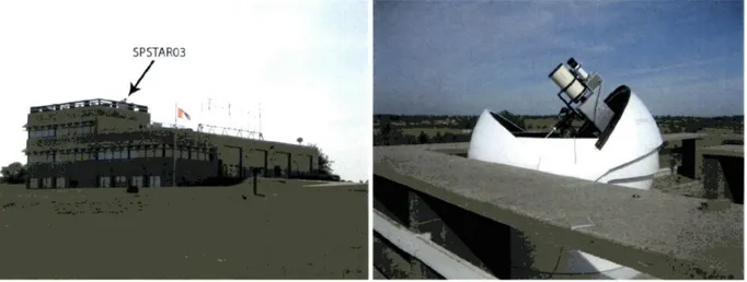
2.3 Research site (Egbert, Ontario)
Egbert (Ontario, Canada, 44°14'N, 79°45'W, UTC-4h)
is located around 80km north of
Toronto and was chosen as an installation site for the SPSTAR03
(Figure 2.1).
^Performing this analysis requires one to implicitly assume temporally stable, homogeneous atmo sphère between the measurement periods.
Egbert represents an excellent choice for the installation and testing of the
starpho-tometer for several reasons. First, Egbert is an active Environment Canada research
center as well as one of the operational sites of the AEROCAN (AERosol CANada)
sunphotometer network. This network is a subnetwork of the world-wide AERONET
network run ont of Goddard Space Flight Center (GSFC)
NASA.
The site hosts a mul
titude of atmospheric research instruments and includes among others a sunphotometer,
lidars and a total sky imager. The analysis of these différent types of measurements,
yields a better understanding of the local aérosol dynamics and thus facilitâtes an évalu
ation of the SPSTAR03 performance. Secondly, Egbert is strategically placed inasmuch as it is influenced by both rural air masses and urban air masses from the nearby citiesof Barrie (20 km to the northeast) and in particular metropolitan Toronto (80 km to
the south). This combined influence allows one to distinguish between background, ru
ral low-level aérosol conditions and elevated aérosol concentrations associated with the
polluted urban air. Finally, according to the AEROCAN statistics, Egbert exhibits the
largest number of cloud-free days in Canada {Freemantle, 2008). These exceptional clear
SPSTAR03
/
Figure 2.1: The starphotometer's location on the roof of the CARE (Center for At-niospheric Research Experiments) building, Environment Canada. Left: location on the
roof, photo source: André Grôeschke. Right: a close-in of SPSTAR03 inside its protective
Chapter 3
Methodology
3.1 Methodological Flow Chart
The methodological flow chart is presented in Figure 3.1.
3.2 Theoretical background
3.2.1 Total optical depth
In the absence of cloud the fraction of light that is scatterered (ont of) and absorbed in
a given direction when light propagates through an atmospheric layer of an infinitésimal
thickness ds is given by:
dôs =
^
=—nis)ds
(3.1)
where /
is the irradiance (power per unit area and per unit wavelength interval) in
a given direction at a point in the atmosphère and k is the extinction (atténuation plus
scattering) coefficient with the units of inverse length (m~^). It is important to note that
the latter quantity is a fondamental property of the médium (i.e. independent of the
light field) representing the fraction of light which will be attenuated per unit distance in
any direction. It is the product of the extinction cross section per particle (the effective
optical area of a single interacting particle) times the particle number density (see Rœs,
2001 for example). The quantities I and k are expected to be wavelength dépendent.
Review of the
existing literature
Installation of the
starphotometer
Optical and polar alignment
Initial tests
Data codèrent with
theoretical expectations^
Mo Yes
Data acquisition at Egbert
Lidar data analysis Extraction and analysis of the sunphotometry data
Extraction and analysis of
the starphotometry data
Corrélation of AOD with
lidar vertical profiles
Day-night continuity analysis
Results and conclusions
Spectral star catalogue or a calibration value Star's extraterrestrial magnitude Star's magnitude measured on the ground It^agnitude différence
1
Total optical depth, ô-p
Estimations of O3, NO2, H2O
Subtraction of
molecular components ÔRay (empirical formula)
Fine (ôx) and coarse
Angstroms exponent,
a
Aérosol optical
depth, 5.., (ô ) mode
thickness ds. Assuming an atmosphère that is horizontally homogeneous and changes its
properties only in the vertical direction, n becornes simply a function of altitude, 2:. We
can then write:
dôg =
^
=—K,{z)mdz =—mdÔT
(3.2)
where dôr =
K{z)dz represents an incrémental measure of the total optical depth
in the zénith direction . Its value between ground level and an altitude ^
(a common
standard in the community);
rz
—
[
ndz
(3.3)
Jo
represents a measure of distance in the atmosphère in nuits of ^
(^ being a measure
of mean free path, the average distance before a given photon is absorbed or scattered).
For a horizontally homogeneous atmosphère, the air mass, m, is simply where 9 is a zénith angle in the direction of the irradiance I. Such a définition of m présumés that a spherical geometry of the atmosphère is not an important factor. This is generally an
acceptable approximation for 9
<
60° (see Thomason et ai, 1983 for a discussion of m).
The differential équation 3.2 is easily solved to yield the Beer-Lambert law {Seinfeld
and Pandis, 1998):
/ = /o (3.4)
where Iq is irradiance at a reference point in the atmosphère. For sun- or
starpho-tometery Iq is the irradiance of the sun or a star outside of the atmosphère and I is the corresponding irradiance at the given altitude (ground level for sunphotometry or
starphotometry).
As irradiance is typically proportional to the signal measured by a photometer, we
can express the Beer-Lambert law in the following way, keeping the original notation of
Leiterer et al, 1995:
Um^Uoe-"^^^
(3.5)
where
Um : measured signal on the ground (volts or digital number)
the atmosphère (volts or digital number)
The value of 5t can be decomposed as {Shaw et ai, 1973):
Sx — ^Ray T
<5^er T
^Ozone +
Sh20 +
Sn02
(3-6)
whereS
Ray- the optical depth of molecular scattering (Rayleigh scattering)
S^er '■ optical depth due to aérosols
Sozcme,^H20,Si<jo2-
the optical depths due to absorption by ozone, water vapor, and
nitrogen dioxide respectively. These three molecular components dominate the molecular absorption in the visible and near infra red (NIR) régions of the electromagnetic spectrum
{Seinfeld and Pandis, 1998).
The following subsections discuss the estimation of each of the individual components of 3.6 when processing starphotometry data. The sunphotometry AOD values employed
in our continuity analysis were obtained directly from the AERONET database (see
section 3.3.1.1 for détails).
3.2.1.1 Rayleigh optical depth, ÔRay
The value of ÔRay can be estimated with the help of an empirical formula derived for
standard molecular profiles {Frôhlich and Shaw, 1980):
.
F • 0.00865 • ^-(3.916+0.074-A+^)
ORay -
5
(3.7)
■M)
Where F is the measured atmospheric pressure, Fq is the standard atmospheric pres
sure at sea level (1013 hPa), and A is the wavelength (in microns).
3.2.1.2 Ozone optical depth, ôozcme
The following équation was employed for the évaluation of the ozone optical thickness
(from Schulz, 2007b):
c
_ ^03 [^3]
o\
àozane- (3-8)
where
koa - spectrally dépendent ozone absorption cross section, , [2.69 x 10^^cnFm.olecule~^]
[O3] - concentration of ozone in Dobson units, DU. 1 DU corresponds to 2.69 x 10^®
molécules of ozone per cm? of atmospheric column for standard température and pressure
(STP)
conditions of T
=
273°K,
P
=
1013 hPa. It physically corresponds to the height of
an atmospheric column of a given gascons constituent if that constituent were compressed to STP conditions.The
coefficients are presented in Table 3.1 {Schulz, 2007a). Ozone absorption is
negligible after 778.5nm.
Table 3.1: Spectral ozone absorption coefficients.
A(nm)
450.9 469.3 500.4 532.7 550.1 605.2 640.4 675.5 750.0 778.5ux
0.003 0.018 0.031 0.065 0.083 0.123 0.079 0.038 0.008 0.0025
No m situ ozone measurements were obtained during the course of this project. In-stead, the values from the Environment Canada daily Ozone Maps were used. These values are mainly derived from ground-based measurements acquired by Brewer
spec-trophotometers. Over areas with poor data coverage adjustments are performed
ac-cording to the satellite observations from NASA's Total Ozone Mapping Spectrometer
(TOMS) (the maps along with their discription can be found at http://exp-studies.
ter.
ec
.gc.
ca/e/ozone/Curr_map.htm, current as of May 21, 2009).
3.2.1.3 Water vapor optical depth, ÔH2O
To eliminate the need for the water vapor compensation, one can choose the spectral
measurement bands where the water absorption is negligible and thus ÔH2O ~ 0. In reality this is not always a good approximation (especially in the case of the certain
infrared bands) and one bas to use a measured value of the water vapor content in order
to estimate 0^20- This was not done in the présent work; the important conséquences
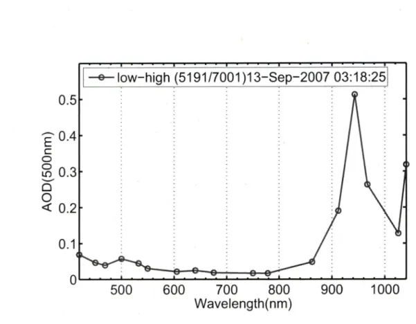
on the estimated AOD in the NIR bands are discussed below. A typical SPSTAR03
spectrum taken on September 13, 2007 at 03:18:25 UTC is presented in Figure 3.2.
The fact that the AOD values in the NIR are larger than those at the smaller
wave-lengths is problematic given that one expects a
type of decrease with wavelength (see
the Angstrom Exponent discussion below). The problems are suspected to be due to the
water vapor (bands 912.1, 943.0 and 967.2nm) and O2-O2 absorption (band 1040.6nm,
Michalsky et ai, 1999). In the sunphotometer case, a water vapor correction is performed
by calculating the value of the water vapor content using the 940nm channel and
0.5
ÊO-4
c os
0.3
Q O < 0.2low-high (5191/7001
)13-Sep-2007
03:18:25
0.1 ©—e 500 600 700 800Wavelength(nm)
900 1000Figure 3.2: Typical spectrum taken by SPSTAR03 on September 13, 2007 shows abnormally elevated AOD values in the NIR part of the spectrum. We note that the label "AOD" is really a misnomer for the bands between 900 and 1000 nm since these
bands were purposely selected for the analysis of water vapour {Grôschke, 2008).
et ai, 1997). A similar strategy could be used in starphotometery. The elevated AOD
at 1040.6nm is thought to be due to the residual O2-O2 with an absorption peak at
1065.2nm.
It should be noted, however, that the abnormally high AOD values in the NIR might
also be of instrumental nature and the problem needs further investigation {Grôschke,
2009).
3.2.1.4 Nitrogen dioxide optical depth,
8^02
Nitrogen dioxide {NO2)
is highly variable in the atmosphère and the values of 8^02 can
change by more than a factor of 100 for an urban location (from less than 0.001 up to
0.175, O'Neill, 1999^). The NO2
cross section peaks at around 400 nm and decreases to
negligible values around 550 nm where the cross section is fï; ^
of the cross section at 400
'The NO2 optical depth estimâtes we give here represent the same wavelength range employed by O'Neill, to wit; "In what follows, the NO2 optical depths are referenced to an absorption cross section
nm. Outside of the big cities, the values are typically less pronouneed and usually do net
exceed 0.01 (idem). In the absence of in situ nitrogen dioxide measurements, we assumed,
in the présent work that NO2 absorption was negligible relative to other uneertainties
associated with the starphotometer measurements.. The neglect of NO2
absorption can
however resuit in some important AOD errors. In the studies by Schroeder and Davies,
1987, for example, the AOD values were reduced by 22, 12, 3
and 1%
(400, 500, 610 and
670nm, respectively) when the N02
absorption was taken into account (for an average
NO2
value of 0.003 atm-cm). It should be noted that these values were obtained for a
medium-sized but relatively high polluted city (Hamilton, Ont.) and are probably less
elevated for a semi-urban site, like Egbert.
3.2.2 Aérosol optical depth, AOD
Aérosol optical depth can be calculated from 3.6 as a différence between the total optical
depth and the sum of the atmospheric components:
^Aer =
St — {^Ray +
^Ozeme +
^H20 +
<^^02)
(3-9)
Its amplitude is predominantly an indicator of aérosol abundance while its spectral
form contains information on particle size and refractive index. This information partition
is determined by the fundamental partition of optical depth into abundance (integrated
number density, Aact) and (vertically averaged) optical cross section (o-^er);
^Aer ~
Aer
(3.10)
3.2.3 Angstrom Exportent
The Angstrom exponent, a {Angstrom, 1964) is another key parameter in sun- and
starphotometery studies. It expresses an approximate dependence of AOD
on the
wave-length and is defined by the fundamental Angstrom relation:
5,
=
/3A-"
. (3.11)
where
5x - AOD at a wavelength A
P
- Angsrom's turbidity coefficient which equals
at A =
Ifxm
The Angstrom exponent provides information about the size of the aérosols with
the higher values of a corresponding to smaller partiale sizes. Typical a values (for
wavelength ranges which extend from the visible to the near IR) range from higher
than 2 for small partiales associated with forest lires or the sub-products of fossil fuel
combustion down to nearly 0
for partiales such as relatively large desert dust or sea sait
aérosols {Eck et al, 1999; Schuster et ai, 2006).
The Angstrom exponent can be calculated from two AOD measurements 5i and 62
by ratioing équation 3.11 at the respective wavelengths of Ai and A2 and taking the
logarithm of both sides. Solving for a yields:a=-—^
(3.12)
In practice a is calculated as a négative slope of a régression between the logarithm
of AOD and the logarithm of the wavelength for several spectral bands (in this work,
aside from the SDA computations described below, we used the range between420.6-862.7nm for the starphotometry data). Once the Angstrom exponent is calculated, it
can be used to estimate optical depth at any wavelength: équation 3.11. It should be noted that the standard Angstrom approach in sunphotometry présumés that spectral
variation is first order in log(AOD) versus log A space. This approximation serves many
useful first order purposes but is known to be inappropriate (especially for certain aérosol
types such as smoke; see Eck et al, 1999). In such cases one must resort to second or
third AOD
spectrometry. This means that the Angstrom exponent becomes wavelength
dépendent and can (probably should) be calculated in a differential calculus fashion at a
single reference wavelength {O'Neill et al, 2001a). This is, as a matter of fact, what is
done implicitly in the application of the SDA algorithm discussed below.
3.2.4 Spectral Deconvolution Algorithm
While the Angstrom exponent 3.11 is a simple and robust indicator of average aérosol di
mensions, it essentially contains a mixture of information from both the fine (submicron)
and coarse (supermicron) mode partiales {O'Neill et al, 2001b). The simple séparation
phenomena related to modeling and radiative transfer proce&ses [O'Neill et al, 2001a).
The fine mode, for example, is dominated by aérosols that resuit mainly from biomass
burning (forests, agriculture, etc.) and anthropogenic pollution (industrial processes,
electricity génération, etc.) The coarse mode,
on the other hand, is associated with
nat-urally produced aérosols such as desert dust (as well as clouds). Assuming a bimodal
particle size distribution one can use the spectral shape of AOD in order to extract the
optical information related to the fine and coarse modes
(idem). This task was performed
with the Spectral Deconvolution Algorithm (SDA)
of O'Neill et ai, 2003. One advantage
in analyzing AOD spectra using this method of optical inversion is that we can
simulta-neously investigate the spectral behavior and the amplitude of the AOD. Moreover, the coarse mode optical depth has proven to be a reliable indicator of the presence of thin
and homogeneous clouds (idem). The SDA was applied to both the sunphotometry and
starphotometry data using 6 wavelengths (380, 440, 500, 675, 870 and 1020nm)
for the
former and 4 wavelengths (420.6, 500.3, 640.4 and 862.7nm)
for the latter.
3.3 Measurement methods
and instruments
3.3.1 Sunphotometry
Ground-based sunphotometry is a means of measuring the extinction of solar radiation
through the atmosphère. The fundamental transmission équation of sunphotometry is
described by the Beer-Lamber law (équation 3.5). By measuring solar intensity on the
ground, Um, and comparing it to the value at the top of the atmosphère, Uo, a value of
the total optical depth, Ôt, is calculated. The sun's angular displacement from the zénith
position is accounted for in terms of the air mass factor, m
(Figure 3.3).
The Langley method is typically used to estimate the extra-terrestrial signal {Shaw et ai, 1973). In this procédure one first obtains a sériés of measurements with a
sunpho-tomer at différent air mass values. Plotting a graph (a Langley plot) that has abscissa
values of m
and ordinate values of In Um yields, in the presence of a stable (fixed AOD)
at
mosphère, a linear dependence whose intercept corresponds to the signal at zéro air mass
(i.e. the signal which would be measured by the instrument outside of the atmosphère).
By referencing this extrapolated signal to the known absolute values of the incident so
lar radiation, one can, if desired, obtain an absolute calibration of the sunphotometer's
Un
0
m
Um
Figure 3.3: Sunphotometry measiirement principle. The used notation is of équation
3.5.
solar flux). As sunphotometers are primarily used to study aérosol optical properties,
the extinction measurements (and Langley plots) are performed at several wavelengths.
An Angstrom analysis can then be applied to give particle size information. There is a variety of modem sunphotometers available that differ in spécifications such as a
num-ber, positioning and width of the spectral bands, detector type, field of view and tracking
style (handheld or automatic). In this work, we used a CIMEL CE-318 sunphotometer
(the standard instrument of the AEROCAN/AERONET network) to obtain day-time
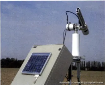
AOD values.3.3.1.1 CIMEL CE-318 Sunphotometer
The CIMEL CE-318 sunphotometer (a typical system is shown in Figure 3.4) is
perma-nently installed at Egbert and has been in opération since 1997.
The CE-318 is actually an automated sunphotometer and sky radiometer that takes measurements of the direct solar radiance in seven spectral bands: 340, 380, 440, 500,
675, 870 and 1020nm^. The instrument also has a 940nm channel dedicated to water
vapor measurements (which are employed to correct for water absorption effects in the other "aérosol" bands). The essential characteristics and the modes of opération of the
CE-318 are presented in détail in Holben et ai, 1998. Raw sunphotometry data from the
^It also acquires sky radiance in the solar alraucanter. However since we did not exploit this capability
in the thesis project we simply refer to it as a sunphotometer. It is also noted that a newer version of
Figure 3.4; The CIMEL CE-318 sunphotometer
photo/, accessed on May 21, 2009.
Source: http://www.cimel.fr/
CE-318 is automatically uploaded to the AERONET database, where it gets processed
according to pre-established protocols (idem). The AOD data products, available using
the AERONET download tool, are processed to several levels . For the day-time AOD values employed in this work we used the Level 1. product for the Egbert site . Level
1.5 corresponds to the data that has been cloud-screened but may not have the final
calibration values applied and is not quality assured (http
:
//aeronet.
gsf
c.
nasa.
gov/
new_web/aerosols.html, accessed on May 20, 2009).
3.3.2 Starphotometry
Starphotometry is similar to sunphotometry inasmuch as both share the same measure-ment principal. The former technique, however, permits the measuremeasure-ment of the irradi-ance from bright stars, rather than from the sun. The basic principle of starphotometry
can be expressed by an équation similar to 3.5. When dealing with stars one often uses
the apparent (log-based) magnitudes from astronomy rather than absolute irradiance
values to characterize the intensity of the radiation flux. Historically, the stars have been separated into several brightness classes or magnitudes. One can define an apparent star
magnitude accurately in ternis of the observed flux density, F
([F] =
Wm''^), by
normal-izing the flux such that magnitude 0 corresponds to some predetermined reference flux
M
=
-2.51ogio^
(3.13)
i'ref
The factor 2.5 cornes from a historical fact; originally the stars were separated into
6 brightness classes, where a star of the first class is approximately 100 (fii 2.5^) times
brighter than a star of the sixth class (idem). Apparent magnitudes as defined in 3.13
are dépendent on the instrument used to measure them and can have différent flux
densities iVe/ corresponding to the magnitude 0
(idem). However, a différence between
two magnitudes Mi and M2 measured with the same instrument is independent of
Fref-(
Fi
Ml- M2 = -2.5 logio logio
^
Fref
Fref J
= -2.51og,„f
(3.14)
i'2
Assuming that a star's flux is proportional to the output U of the starphotometer's
detector, we can rewrite équation 3.13 as:
M=-2.51ogioT^
(3.15)
Uref
where U and Uref are the signais in digital number counts corresponding to the
measured and reference fluxes respectively. Adopting this définition, the Beer-LambertLaw 3.5 can be rewritten in a following form {Leiterer et ai, 1995):
M
=
Mo
+1.086-St-m
(3.16)
where
M - measured magnitude on the ground
■ Mo - extra-terrestrial magnitude
m - air mass
the factor 1.086 in 3.16 comes from the multiplication 2.5 • loge.
There currently exist two methods to obtain the optical depths (and consequently
aérosol optical depths using 3.9) from the starphotometry measurements: a two-star
method, TSM {Leiterer et ai, 1995) and a more recent one-star method which is the
analogue to classical sunphotometry, OSM
{Herber et ai, 2002).
3.3.2.1 Two-star method
The differential two-star method, depicted in Figure 3.5, is based on the measurement of
two bright stars (labelled 1 and 2) having a substantial air mass différence. In the figure
Mi and Mo t are the stars' measured and extra-terrestrial magnitudes, respectively, nrii represent the air mass and hi the élévation of star i.
mMoi
M
mMo2
hh
Mi
M2
Figure 3.5: Two-star measurement principle with starphotometry.
The use of two stars is important (if not necessary) as it is difficult to estimate the
instrument's extraterrestrial signal {Leiterer et ai, 1998). Due to the Earth's rotation
around the sun and about its own axis, the stars available for measurements change depending on the time of the day and the time of the year. Accordingly, one of the principal difficulties associated with the Langley procédure in starphotometry is that the
analysis has to be performed for multiple stars to ensure continuous observations {Pérez-Ramirez et al, 2008b). Another problem is that at high altitudes, like in the Arctic, the
air mass of a particular star changes much slower than the atmospheric conditions and
the Langley procédure is also inapplicable {Herber et al, 2002).
Using the relationship 3.16 for each of the two stars and subtracting one équation from another, yields:
A'/j — M2
— Mqi — Mq2 T
1.086 •
— ^^2)
Solving 3.17 for ôx yields:
^ _ 1 (Ml — M2) — (Mqi — M02)
.
^
1.086
mi —1712
The fundamental hypothesis of équation 3.18 is that the normalized optical depth is the same for the two stars (that St = ^ri = An atmosphère that is horizontally homogeneous would satisfy this condition. Equation 3.18 also indicates that only the ratio
(équivalent to the logarithmical différence, see équation 3.14) between the two signais on
the ground and outside of the atmosphère is required to estimate 5t- Fundamentally,this means that multiplicative instrumental influences cancel ont and it is not necessary
to calibrate the starphotometer in order to establish Mqi — M02 =
log (^)- One could
instead use the extraterrestrial star magnitudes, Mo, obtained from the astronomicalcatalogues. In this work we used the widely-cited catalogue by Alekseeva et al, 1996
for its comprehensive star archive, stated accuracy of measurements as well as spectral resolution. Finally, équation 3.18 nécessitâtes to define a minimal air mass différence,
Am = mi — 1712, for which the method still produces reliable results. For the discussion on the Am used in this work, refer to section 3.3.2.5.
3.3.2.2 One-star method
For the one-star method (GSM),
one flrst has to establish an extraterrestrial calibration
constant. Moi (i for instrumental) -
the magnitude that the instrument would measure
outside of the atmosphère (Figure 3.6).
The calibration values for the GSM can be derived from the TSM data as proposed
by Herber et ai, 2002. To achieve this, one chooses a night with stable atmospheric
conditions and collects a sériés of 5t measurements with the TSM using a particular star
pair (équation 3.18). An average Sx value for the period is then obtained and used in
3.16 to calculate Mo, for each individual star:
Moi = Mi- 1.086-ÔT-m (3.19)
It was shown that the Langley calibration procédure (described in section 3.3.1) could
also be used successfully to obtain a star's extraterrestrial values {Pérez-Ramirez et ai,
2008b). But apart from the issue of multiple stars for which the calibration has to be
performed (see section 3.3.2.1), the Langley method requires atmospheric stability that
^to minimize the inhoniogeiieity effects, the two measurements are taken as close as possible to one
m
h\
1^VI
1
1
1 11
Figure 3.6: One-star ineasurement principle with starphotometry. The notation is of Figure 3.5.
can usually be achieved only at a high-altitude site (idem). For this reason the OSM calibration values used in this work were derived from the TSM data.
Once the Moi values are established, it is possible to calculate the optical depth, 6t,
with one star:
Ôt —
Mi - MfOi 1.086 • m
3.3.2.3 Sensitivity of the Two-star method
(3.20)
While the TSM method is based on the inherent assumption of a horizontally homoge-neous atmosphère, real atmospheric conditions exhibit some degree of inhomogeneity . It is then expected that AOD values obtained using the TSM will be sensitive to changes
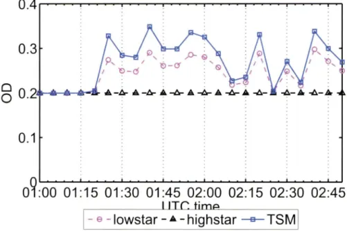
in the measured star magnitudes of Mi and M2 which are not due to nominal homoge-neous différences. It can be instructive to investigate the sensitivity through the means of Figure 3.7.
In the hypothetical scénario of Figure 3.7 we assume that during a particular night, the
irradiances of two 'low' and 'high' stars (with lower and higher élévation respectively)
are initially measured for the same stable atmospheric conditions (time period 01:00-01:15). Given the assumption of correct calibration values, the two respective OSM signais (équation 3.20) and the TSM signal (équation 3.18) yield the same value of 0.2
o 0.3 A ! N >■ -A
A ^
N A O- -G -0-3-O -o -O— 0.1 01:00 01:15 01:30 01:45 02:00 02:15 02:30 02:45 I ITP. timp-® -lowstar
highstar -a-TSM
Figure 3.7: Modelled perturbations in the TSM signal, produced by the OD variations of the high star. TSM déviations from the nominal OD=0.2 are comparable to or less tlian the déviations of the high star. The air mass of the high star changes from 1.0862
at 01:00 to 1.5367 at 02:50.
stable for the duration of the night, while at 01:15 a hypothetical thin cirrus cloud, with a variable cloud optical depth (COD) between 0 and 0.1, is advected in front of the high star. From 01:15 on, we can express the time variations of the low and high optical depths as:
ODiowit) = OD = 0.2 and ODhighii) = OD + COD{t), where 0 < COD{t) <0.1
By calculating the observed star magnitudes corresponding to ODiow{t) and ODhigh{i)
and substituting them into équation 3.18, a corresponding TSM signal can be estimated(curve 'TSM' in Figure 3.7). As can be seen, the variations in the TSM values are
anti-correlated with the variations in the OD values of the high star which are in turn due to the presence of the cloud. The TSM déviations from the nominal OD of 0.2
are comparable or less than the déviations of ODhigh{i)- Figure 3.8 présents a différent
scénario in which the high star has stable observation conditions and low star is affectedby a cloud:
ODiow{t)
=
OD
+
COD{t) and ODhigh{t) =
OD
=
0.2, where G <
COD(t)
<
0.1
0.3 p-Q 0.2 A A A ar O 01:00 01:15 01:30 01:45 02:00 02:15 02:30 02:45 I ITP. timp
- © -lowstar
highstar
TSM
Figure 3.8: Modelled perturbations in the TSM signal, produced by the OD variations of the low star. TSM déviations from the nominal OD=0.2 are greater than the déviations of the low star. The air inass of the low star changes from 2.3072 at 01:00 to 5.5265 at
02:50.
In Figure 3.8 the TSM variations are, in this case, correlated with the variations in
OD
of the single (low) star, but the déviations from OD=0.2
are greater than in the case
of the high star. In général, it can be shown from the équations 3.18 and 3.20 that with
the other parameters held constant, a star with a greater air mass, m, (lower élévation),
produces greater perturbations in the TSM signal.
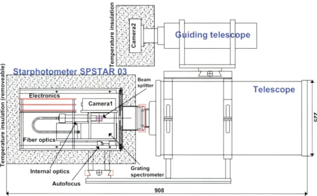
3.3.2.4 SPSTAR03 starphotometer
The SPSTAR03 starphotometer was developed by a German company (Dr. Schulz and Partner GmbH). The principal components of this instrument are depicted in Figure 3.9. These include a Maksutov telescope (aperture/focal length 180mm/1800mm) to collect
star light, a Losmandy Gll equatorial mount for précisé star tracking, a viewfiender
a star's image on the measuring diaphragm and finally a measuring unit containing a grating spectrometer, a CCD detector and other secondary optics.
Guiding caméra Cantertng caméra, CCD detector and computer interface Mount and mount controller Viewflnder Telescope Jt:
%
Figure 3.9: Principal components of SPSTAR03 starphotometer.
A schematic diagram of the SPSTAR03 is shown in Figure 3.10. Initially, the instru
ment is pointed towards a certain star with the help of the Losmandy G11 mount. The
stellar light is captured by the primary (caméra 1) and guiding (caméra 2) telescopes and
is directed to the measuring unit and caméra 2 respectively. Inside the measuring unit,
the light is divided by a beam splitter and approximately 10% of the signal is directed
towards caméra 1. Both caméras 1 and 2 are used to center the star's image in the middle of the detector. The rest of the light is guided onto the grating spectrometer where it is spectrally separated and subsequently measured by the CCD detector.
The SPSTAR03 signal is measured using a Hamamatsu S7031 CCD sensor that
trans-forms the star's intensity into digital numbers (DN). The DN value is adjusted to take into account the dark current (an electronic signal generated in the absence of incoming
light) as well as the background irradiance of the sky^ and is subsequently transformed
Ciuiding telesc:ope 'J. >î ;v5-> v> V- v'; i ■■('■■ '■
iipiililw
.y-* «■■ ;- ';.v'> ■: <- > .v,--.r v-.. mr;5 'J'. .-- iv'î Telescope ElectronicsM;f:
Cameraln
n
rU",E
mc
ïï
ïï
t -T^r. v';j- Fiber opticstm
K•-Internai optics /
spTcTrometer
Autofocus
908
Starphotometer SPSTAR3 with Telescope and Guiding Telescope (without Viewfinder)
Figure 3.10: SPSTAR03 schematical diagram. Source: K.-H. Schulz
into an apparent star magnitude (A/) using équation 3.15.
The SPSTAR03 takes measurements of the spectral radiance in 17 bands: 420.6, 450.9, 469.3, 500.3, 532.7, 550.1, 605.2, 640.4, 675.5, 750.0, 778.5, 862.7, 912.1, 943.0, 967.2, 1025.6 and 1040.6nm. It should be mentioned, however, that due to the difficulties in the NIR part of spectrum (discussed in the section 3.2.1.3) we chose to limit the analysis in this work to wavelengths up to and including 862.7nm. When in the TSM mode, the measurements are taken in so-called "triplets". Each such triplet consists of a star
brightness measurement of a lower élévation ("low" star), a higher élévation star ("high"
star) and hnally of the low star again. This allows one, by evaluating the différence between the "low-high" and "high-low" pairs of measurements, to check the stability of the atmospheric conditions. For a stable, horizontally homogeneous atmosphère this
différence should be minimal.
The temporal resolution of the instrument, when in the TSM mode, is associated with the measurement time of a single triplet. This time is around 5 minutes depending on
the speed of the stellar centering procédure in the measuring diaphragm. More détails
on the design of the instrument can be found in {Schulz, 2007b).
3.3.2.5 Measurement stars and TSM limitations
The measurement stars for SPSTAR03 are taken from the catalogue of the Bright Stars
for which the extraterrestrial values could be found in Alekseeva et ai, 1996. A sélection
of the Bright Stars is listed in Appendix A, but not ail of them are available for
mea-surements. A choice of stars for a particular night dépends on several factors: operator's
geographical location, tiine of the year (Earth's position around the Sun),
local obstacles
such as buildings or trees, phase/brightness of the moon, star brightness and élévation, etc.
Furthermore, the two-star method, as defined by équation 3.18, imposes other limi
tations in regard to the choice of the measurement pairs. The principal condition is for
the stars to have a sufficient air mass différence Am = rrii— TO2 in order to avoid an ex cessive Ôt sensitivity to the observational changes in each individual star. Leiterer et ai,
1998 suggest 1 < Am < 3 while Herber et ai, 2002 mention the following conditions;
mi >
2.9, m2 <1.4
(élévation values of 20° and 45° respectively converted to air masses
using m =
sin{eielaticm)^'
work, we used the default condition of the
measuring software Am >1.0 (Schulz, 2007) with the average and maximum values forthe total measurement period (including both 2007 and 2008 datasets) being 1.9 and 5.3
respectively. Besides the air mass condition, the stars should at least be in the same part
of the sky to minimize the inhomogeneity effects. This was ensured by maintaining the
maximum allowable azimuth différence of 90° between the stars (idem).
Several star pairs need to be used to satisfy ail of the above requirements given the
apparent movement of the stars during the night. In the beginning of a measurement period, the available stars are carefully studied in the context of the local conditions. Several candidate pairs are set up and those containing the brightest stars are used for
measurements. A sequence of measurement pairs is determined and tried to be kept the
same on the night to night basis. Some adjustments, however, are usually required due
to various factors such as clouds or operational difficulties. For the measurement stars
3.3.3 Lidar Measurements
An atmospheric lidar (LIght Détection And Ranging) is a ranging system that opérâtes
in the optical and near IR part of the spectruin to retrieve vertical profiles of atmospheric
properties. Modem lidar technology fias its origins in 1960s shortly after the invention of the laser (for a fundainental description of lidars see for example Hinkey, 1976; Measures, 1984; Weitkamp, 2005) Its operating principles, which are similar to (microwave) radar,
are snmmarized in Figure 3.11. A
laser piilse is emitted into the atmosphère (1) where, in
addition to the absorption processes, it is scattered in ail directions and at every altitude
by the various atmospheric constituents (2). Some light gets scattered directly back to the ground and is collected by the receiver (3) which includes a telescope and highly
sensitive photodetectors. Transmitted signal Laser emitter
3
\7
Atmospheric constituents Backscattered signal TelescopeFigure 3.11: Lidar operating principle. (1) A laser puise is emitted into the atmosphère; (2) in addition to the absorption processes, the light is scattered in ail directions by various atmospheric constituents; (3) some of the light is scattered directly back to the
ground where it is collected by the receiver optics.
Range information is provided by measuring the delay between the transmitted and received signais. Lidars are well-known for their very high spatial resolution where
scat-tering from an air parcel of a few cubic meters can be detected from a range of tens of
the lidar équation.
3.3.3.1 Lidar équation
For a particular wavelength, the power P
received from a distance R
can be written in
terms of the lidar équation
(
Weitkamp, 2005):
F{R)
=
KG{R)p{R)T{R)
■
_
(3.21)
where
K - performance constant of the lidar system
G{R)
- quantity that describes the range-dependent measurement geometry
P{R)
- backscatter coefficient at a distance R
T{R)
- transmission to distance R
and back
The parameters K and G(R)
are completely determined by the lidar setup and are
known a priori. AU the information about the atmospheric parameters is contained in
P{R)
and T(R). The backscattering coefficient P{R)
détermines the strength of the return
lidar signal and describes how much light is scattered into the backward direction (région 3
in Figure 3.11). Assuming that the light is scattered mostly by air molécules (index 'mol')
and aérosols (index 'aer') {Carswell, 1983; Weitkamp, 2005), we can correspondingly
express P{R) as:P{R)
=
PmoliR)
+
PaeriR)
(3-22)
The transmission factor T(R)
in 3.21 represents the fraction of light that is attenuated
while propagating to the scattering volume and back:R
T{R) = exp(—2 j
K{r)dr)
(3.23)
0
Where k - extinction coefficient, describing the combined capacity of ail the
encoun-tered particles to diminish the laser beam intensity. The extinction occurs because of
the scattering (other than in the backward direction) (index 'sca') and absorption (index
'abs') of light by molécules and aérosols and we can thus express k as :
where k was defined in équation 3.1 and the séparation into components is coherent
with équation 3.6. The main problem associated with équation 3.21 is that it relates pro
files of one measured quantity, P(R), to profiles of two unknowns, namely backscattering
coefficient P{R)
and extinction coefficient k{R). In order for the équation to be solvable,
one needs to make certain assumptions regarding the relationship between p{R)
and k{R)
and this is done with the lidar ratio (also known as the extinction to backscatter ratio):
7-/p\ _ ^(-^)
. T (]D\ _ '^rnoljR) . J /m _ l^aeriR)
1^261
"
m)
'
"
PmoliRY
^ PaeriR)
^ ^ ^
where
r f r)\
PaerLaer T
YmolLmol
/o o<î^
While the molecular lidar ratio, Lmoi can be determined from Rayleigh scattering
theory (eg. Bodhaine et al, 1999), the values of the aérosol lidar ratio, Laer are dépendent,
to a degree, on particle size, shape and refractive index (particle type) and must be
estimated (e.g. Cattrall et ai, 2005). Thus the accuracy of the derived Paer{R) profiles
obtained with the lidar équation 3.21 is dépendent on the accuracy of the estimated lidarratio 3.25.
3.3.3.2 AOD estimâtes from the lidar profile
One can estimate ôaer Rom the values of /?aer by using the following reasoning. If the
lidar is zénith pointing, the R dependencies can be replaced by z dependencies, i.e.
Paer{R)
=
Yaer{z) aud Kaer{R) =
i^aeri^)- We
theu uote that the backscattering coefficient
fdaer cau be expressed as:
n
^
Paer
(cOSTr)
Paer — ^aer,scatPaer(cOSTr)
— I^aer ^O.aer . yo.Zlj
Att
where
«■aer,scat " scatteriug coefficient (fraction scattered per unit length; c.f. the définition of
extinction coefficient above);
- fraction of radiation scattered by aérosols into the direction which is opposite
to the incidence direction (180° scattering angle) per unit solid angle. The quantity p^r
is called the scattering phase function (see Hansen and Travis, 1974, for example).
Rearranging yields:
= p,,,(cosi80°) '^0 47
The lidar ratio of équation 3.25 is accordingly:
Laer =
= p„„.(cos 180°)
fJaer Uq
Assuming that Laer is independent of height (i.e. Laer{z) =
Laer) and using 3.29 one
arrives at:^aer — J l^aeri,z)dz — J
(daeri^z) Laer(^z)dz — Laer j
Paer(^z)dz
(3.30)
0 0 0
Once the /0aer-profiles are derived, they can be integrated over the entire atmosphère
and multiplied by a suitable lidar ratio to yield an approximation for the aérosol optical
depth. The différence in the line of sight between the lidar and starphotometer, however,
can resuit (depending on the degree of horizontal inhomogeneity in the atmosphère) in
moderate to signifîcantly différent results depending on the star choice (low or high).
The measurements associated with the high star, being nearest to the lidar zénithal line
of sight, should logically be better correlated with the lidar data results.
3.3.3.3 ALIAS
The ALIAS (Aérosol Lidar for Atmospheric Studies) is a zenith-pointing lidar that was
conceived for the analysis of the long range transport of air masses. ALIAS supplies atmospheric profiles of aérosol backscattering coefficients, paeri at 532 and 1064nm. These profiles provide an optical measure of vertical aérosol loading in the atmosphère and can be used to qualitatively validate starphotometry data (with a particular test being a Visual analysis of the corrélation between SDA coarse mode optical depth and thin cloud profiles detected by ALIAS). Moreover, the vertically integrated Paer hdar signal should, given the assumptions leading to 3.30, be proportional to the aérosol optical
depth (see the discussion in O'Neill et ai, 2004 for example). Consequently, a corrélation
analysis between the ALIAS
integrated extinction coefficients and the optical depth values
obtained with the SPSTAR03 can serve as an additional, quantitative assessment of theChapter 4
Principal results obtained
4.1 Summary of the data obtained
During the periods of August 30-September 20, 2007 and June 30-July 5, 2008 a sériés of optical measurements were carried ont with three différent instruments at Egbert; the CIMEL CE-318 sunphotometer, the SPSTAR03 starphotometer and ALIAS. An overview of the measurement periodsd is presented in Table 4.1 and the analysis of each type of data is discussed in the following sections. AU date and time values in this work are
referenced to coordinated universal time (UTC).
Table 4.1: Summary of measurements obtained at Egbert. Filled cells represent data
collection dates. 2007 2008
Aug
30
Aug
31
Sep
1
Sep
2
Sep
3
Sep
4
Sep
9
Sep
01
Sep
12
Sep
13
Sep
14
Sep
17
Sep
81
Sep
19
Jun 30
Jul
1
Jul
2
Ju l
3
Jul
4
Jul
5
Sunphotometry 1 M1
1
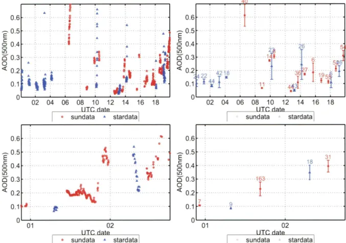
Starphotometry p ?... - > "7*1 1 P ■ . ■ ALIAS lidar 1 1 14.2 Starphotometry and night-time lidar data
The combined datasets for Aug 31-Sep 4 as well as Sep 10, 13 and 19, 2007 are presented in Figure 5.3. These dates were constrained by the availabilty of lidar data and represent