HAL Id: pastel-00003177
https://pastel.archives-ouvertes.fr/pastel-00003177
Submitted on 17 Dec 2007HAL is a multi-disciplinary open access archive for the deposit and dissemination of sci-entific research documents, whether they are pub-lished or not. The documents may come from teaching and research institutions in France or abroad, or from public or private research centers.
L’archive ouverte pluridisciplinaire HAL, est destinée au dépôt et à la diffusion de documents scientifiques de niveau recherche, publiés ou non, émanant des établissements d’enseignement et de recherche français ou étrangers, des laboratoires publics ou privés.
virtuels : application au P. pinaster dans le plan LR
José Xavier
To cite this version:
José Xavier. Identification de la variabilité des rigidités du bois à l’intérieur de l’arbre par la méthode des champs virtuels : application au P. pinaster dans le plan LR. Sciences de l’ingénieur [physics]. Arts et Métiers ParisTech, 2007. Français. �NNT : 2007ENAM0030�. �pastel-00003177�
Ecole doctorale n° 432 : Sciences des Métiers de l’Ingénieur
T H È S E
pour obtenir le grade de
Docteur
de
L’École Nationale Supérieure d’Arts et Métiers
Spécialité “Mécanique”présentée et soutenue publiquement par
José XAVIER
le 27 novembre 2007IDENTIFICATION DE LA VARIABILITÉ DES RIGIDITÉS
DU BOIS À L’INTÉRIEUR DE L’ARBRE
PAR LA MÉTHODE DES CHAMPS VIRTUELS :
APPLICATION AU P. PINASTER DANS LE PLAN LR
Directeur de thèse : Fabrice PIERRON Co-encadrement de la thèse : Stéphane AVRIL
Jury :
M. Rémy MARCHAL Professeur, ENSAM, Cluny Président M. Joseph GRIL Directeur de Recherches CNRS, LMGC, Montpellier Rapporteur M. Jérôme MOLIMARD Maître Assistant HDR, ENSM, Saint-Étienne Rapporteur M. Stéphane AVRIL Maître Assistant HDR, ENSM, Saint-Étienne Examinateur M. José MORAIS Professeur, UTAD, Vila Real (Portugal) Examinateur M. Fabrice PIERRON Professeur, ENSAM, Châlons-en-Champagne Examinateur M. Frédéric ROUGER Directeur de Recherches, FCBA, Paris Examinateur
Laboratoire de Mécanique et Procédés de Fabrication ENSAM, CER de Châlons-en-Champagne
L’ENSAM est un Grand Établissement dépendant du Ministère de l’Éducation Nationale, composé de huit centres : AIX-EN-PROVENCE ANGERS BORDEAUX CHÂLONS-EN-CHAMPAGNE CLUNY LILLE METZ PARIS
Ecole doctorale n° 432 : Sciences des Métiers de l’Ingénieur
Ph.D. THESIS
to obtain the grade of
Doctor
of the
École Nationale Supérieure d’Arts et Métiers
Speciality “Mechanics”presented by
José XAVIER
the November 27th, 2007CHARACTERISATION OF THE WOOD STIFFNESS
VARIABILITY WITHIN THE STEM
BY THE VIRTUAL FIELDS METHOD:
APPLICATION TO P. PINASTER IN THE LR PLANE
Ph.D. Advisors: Fabrice PIERRON Stéphane AVRIL
Jury:
M. Rémy MARCHAL Professeur, ENSAM, Cluny Chairman M. Joseph GRIL CNRS Research Director, LMGC, Montpellier Referee M. Jérôme MOLIMARD Assistant Professor, ENSM, Saint-Étienne Referee M. Stéphane AVRIL Assistant Professor, ENSM, Saint-Étienne Examinator M. José MORAIS Professeur, UTAD, Vila Real (Portugal) Examinator M. Fabrice PIERRON Professeur, ENSAM, Châlons-en-Champagne Examinator M. Frédéric ROUGER Research Director, FCBA, Paris Examinator
Mechanical Engineering and Manufacturing Research Group ENSAM, CER de Châlons-en-Champagne
L’ENSAM est un Grand Établissement dépendant du Ministère de l’Éducation Nationale, composé de huit centres : AIX-EN-PROVENCE ANGERS BORDEAUX CHÂLONS-EN-CHAMPAGNE CLUNY LILLE METZ PARIS
Recomeça... Se puderes,
Sem angústia e sem pressa. E os passos que deres, Nesse caminho duro Do futuro,
Dá-os em liberdade. Enquanto não alcances Não descanses.
De nenhum fruto queiras só metade. E, nunca saciado,
Vai colhendo
Ilusões sucessivas no pomar. Sempre a sonhar
E vendo, Acordado,
O logro da aventura.
És homem, não te esqueças! Só é tua a loucura
Onde, com lucidez, te reconheças. Miguel Torga, Diário, XIII, pág.20.
En premier et avant tout, je voudrais remercier chaleureusement Fabrice Pierron et Stéphane Avril, pour l’encadrement de cette thèse. Votre étonnants connaissances ont été fondamentales pour le bien déroulement de ce travail. Je vous remercie aussi pour l’amitié qui a fleuri entre nous comme résultat de cette thèse.
Queria também agradecer a José Morais pelo seu suporte e troca de impressões ao longo de todo este trabalho. E, nomeadamente, por me ter incentivado, já faz algum tempo, para este mundo da investigação.
Je tiens aussi a remercie Joseph Gril et Jérôme Molimard d’avoir acceptés d’être rapporteurs de ma thèse, Rémy Marchal d’avoir bien voulu présider le jury lors de ma soutenance de thèse, et Fréderic Rouger d’avoir acceptés d’être parmi les membres du jury. Je voudrais remercier à toutes les personnes du LMPF/ENSAM pour la bonne ambiance qu’a toujours entourée pendant mon séjour au labo. Merci pour votre accueil et ouverture, et pour tous ces champs réels d’amitiés qui resteront gravé dans les beaux souvenirs de ma mémoire.
Gostaria de agradecer aos colegas e amigos Marcelo Oliveira e João Luís Pereira do Departamento de Engenharias de Madeiras da Escola Superior de Tecnologia de Viseu pela sua contribuição na preparação dos provetes ensaiados neste trabalho.
A special thanks also for our friend Marie Kelly for her advises concerning the thesis writing.
Agradeço calorosamente à minha família e amigos pelo seu apoio e encorajamento ao longo de todos estes anos. À Sandra, em particular, agradeço o seu amor e atenção, os ingredientes que adocicaram a minha estadia por estas terras gaulesas.
Finalmente, queria agradecer à Fundação para a Ciência e Tecnologia o suporte financeiro sem o qual não me teria sido possível desenvolver este trabalho.
Le matériau bois est un composite naturel produit par l’arbre. Puisque l’arbre con-stitue une ressource disponible sur la Terre, historiquement, le bois a toujours joué un rôle important comme matériau (p.-ex., pour la construction). Dans les dernières décennies, de nouveaux produits à base de bois ont été développés, tel que le bois lamellé-collé ou le contre-plaqué. Ces produits ont été spécialement conçus pour répondre à des exigences structurales (Williamson, 2002). Ainsi, le bois massif et ses produits dérivés sont de nos jours d’une importance considérable, d’autant plus pour les raisons suivantes (STEP,
1996) : (1) les arbres sont produits par une source d’énergie gratuite (le soleil) et sont re-nouvelables et recyclables ; (2) il y a des ressources forestières importantes sur Terre ; (3) la sylviculture et la transformation du bois ont un coût relativement faible ; (4) le bois a une rigidité spécifique excellente. Néanmoins, pour une utilisation efficace du bois dans des applications d’ingénierie, les paramètres matériaux figurant dans les lois de comportement (p.-ex., les paramètres de rigidité dans le modèle élastique linéaire anisotrope), de même que d’autres propriétés telles que les résistances, doivent être correctement caractérisées (ASTM D143,1994; Bodig and Goodman, 1973).
La grume d’un arbre peut être modélisée comme un matériau orthotrope cylindrique (Guitard, 1987; Smith et al., 2003). Trois plans de symétrie sont localement définis par les directions longitudinale (L, 1), radiale (R, 2) et tangentielle (T, 3) des cellules du bois (les trachéides pour le bois résineux). Les propriétés mécaniques du bois sont habituelle-ment identifiées dans ce repère matériau. Le comportehabituelle-ment mécanique du bois peut être analysé à différentes échelles. À l’échelle macroscopique, le bois sans défaut (c.-à-d., le bois sans noeud ou autres caractéristiques structurelles et avec un fil droit) est normalement considéré comme un matériau continu et homogène. Différentes lois de comportement ont été proposées dans la littérature pour modéliser le bois sans défaut, chacunes d’entre elles se limitant à un domaine de validité particulier. Négligeant une possible déformation engendrée par des effets hygro-thermiques, les lois de comportement généralement ad-mises sont les modèles élastiques et viscoélastiques linéaires (Dinwoodie, 2000; Guitard,
1987; Holmberg et al., 1999; Kollman and Côté Jr., 1984; Smith et al., 2003). Le bois semble être décrit plus exactement par un modèle viscoélastique puisque des observations expérimentales ont indiqué une dépendance de la déformation avec le temps. Cependant, pour la plupart des applications pratiques, la déformation dépendante du temps peut
être négligée et le bois peut simplement être considéré comme élastique linéaire. Cette théorie est valide pour des niveaux relativement bas de contrainte (en dessous de la lim-ite d’élasticité), appliqués sur une période courte (quelques minutes) et à température ambiante.
Pour caractériser les paramètres de comportement de la loi élastique linéaire, on utilise des essais mécaniques quasi-statiques. Cependant, en raison de l’orthotropie de la struc-ture du bois, plusieurs essais indépendants sont habituellement employés pour sa carac-térisation mécanique (Guitard, 1987). Ces méthodes se fondent sur des conditions de chargement simples (traction, compression, cisaillement ou flexion) pour lesquelles un état de contrainte simple est supposé s’appliquer sur un élément représentatif de volume du matériau à l’échelle de l’étude. Pour ces essais, une solution analytique peut être obtenue, liant directement les mesures de force et de déformation aux paramètres matéri-aux inconnus. En raison de l’anisotropie et de l’hétérogénéité, la nécessité d’améliorer les essais mécaniques pour l’identification a depuis longtemps fait l’objet d’études (Jones,
1999; Tarnopol’skii and Kulakov, 1998). Dans ce domaine de recherche, plusieurs essais mécaniques ont été conçus et améliorés (p.-ex., l’essai de traction hors-axes et l’essai de cisaillement d’Iosipescu). Néanmoins, quelques inconvénients ont été indiqués pour ces méthodes, à savoir la difficulté pratique de générer un état simple de déformation sur la totalité de la région d’intérêt en raison des effets de conditions aux limites (Grédiac,1996;
Tarnopol’skii and Kulakov, 1998).
Pour l’identification de paramètres de comportement représentatifs d’une essence de bois, plusieurs éprouvettes, prélevées à différents endroits dans différents arbres, sont nécessaires afin de prendre en compte la variabilité structurale inhérente du matériau (Bodig and Goodman, 1973). Ainsi, en raison de l’anisotropie et de la variabilité du bois, on peut conclure qu’un nombre significatif d’essais est requis, ce qui implique un coût important. Pour simplifier cette procédure, une approche a été proposée depuis les premiers travaux de Bodig and Goodman (1973). Sur le fond, elle consiste à établir des rapports entre les différentes propriétés du bois. Puisque le module élastique longitudinal est connu pour la plupart des essences, ce paramètre a été souvent pris comme variable indépendante (Bodig and Goodman,1973;Green et al.,1999;Sliker,1985,1988;Sliker and Yu, 1993). L’évaluation des paramètres élastiques à partir des propriétés physiques, telles que la densité, a également fait l’objet de plusieurs études (Bodig and Goodman, 1973;
Gibson and Ashby, 1997; Guitard, 1987; Sliker and Yu, 1993; Walton and Armstrong,
1986). Un autre type d’approche est proposé dans ce travail.
Grâce au développement des méthodes optiques, permettant de mesurer des grandeurs cinématiques (p.-ex., déplacement, pente, déformation ou courbure) sur toute une région d’intérêt, une nouvelle voie de caractérisation des matériaux s’est développée (Grédiac,
1996, 2004). L’idée fondamentale est qu’une seule éprouvette peut être chargée de telle manière que plusieurs paramètres soient simultanément impliqués dans sa réponse
mé-canique, engendrant des champs de déformation complexes et hétérogènes. En admet-tant que ces champs soient mesurés par une méthode optique appropriée, l’ensemble des paramètres de comportement peut alors être déterminé par une méthode d’identification adaptée. Cette approche semble être particulièrement intéressante pour un matériau comme le bois. En effet, elle a déjà été appliquée au bois et à ses produits dérivés par quelques auteurs (Cárdenas-García et al., 2005; Foudjet et al., 1982; Jernkvist and Thu-vander,2001;Le Magorou et al.,2002; Rouger, 1988).
Le travail présenté dans cette thèse concerne une approche d’identification inverse per-mettant la caractérisation des paramètres de rigidité longitudinale-radiale, (L, R) ≡ (1, 2), du pin maritime (Pinus pinaster Ait.). En particulier, la procédure proposée est basée sur l’application de la méthode des champs virtuels (MCV) à une éprouvette rectangu-laire chargée dans le montage d’Iosipescu. Cette méthode est fondée sur les équations fondamentales de la mécanique des solides déformables : le principe des travaux virtuels (PTV) (qui décrit l’équilibre global d’un corps) et la loi de comportement (qui établit le rapport entre les états de contrainte et de déformation en chaque point d’un solide). Des champs virtuels spéciaux par morceaux optimisés (vis-à-vis du critère de sensibilité au bruit) ont été employés. L’essai a été conçu de telle manière que la géométrie et les conditions de chargement génèrent des champs hétérogènes de déformation. Ces champs de déformation, nécessaires dans le problème de caractérisation du matériau, ont été dé-duits des champs de déplacements mesurés par la méthode de grille, par une approche de régression polynômiale au sens des moindres carrés. Les champs de déformations et la force résultante (mesurée par une cellule de force montée sur la machine d’essai) ont été traités par la MCV pour obtenir l’identification directe des quatre rigidités du bois sans défaut dans le plan LR: Q11, Q22, Q12 et Q66. Ensuite, une contribution à l’évaluation
de la variabilité spatiale des paramètres de rigidité au sein de la grume de l’arbre est présentée.
Le mémoire de thèse est composé de six chapitres. Dans le chapitre 1, une étude bib-liographique sur le comportement linéaire élastique du bois est présentée, avec un intérêt particulier porté aux essais mécaniques habituellement utilisés pour la caractérisation. Des méthodes optiques de mesure des champs cinématiques utilisées en mécanique expérimen-tale et leur intérêt pour la mécanique du bois font l’objet du chapitre 2, ainsi qu’une présentation des essais statistiquement indéterminés et le principe général de la MCV. L’approche d’identification inverse proposée dans ce travail est présentée au chapitre 3. La validation numérique et expérimentale de cette approche sont étudiées aux chapitres 4 et 5, respectivement. Le chapitre 6 décrit l’application de la méthodologie proposée pour caractériser la variabilité spatiale des paramètres de rigidité du bois à l’intérieur de la grume de l’arbre. Enfin, les conclusions générales et quelques directions pour les travaux futurs sont données.
Les principaux résultats de cette thèse sont les suivants.
(i) L’approche d’identification inverse proposée a été premièrement validée d’un point de vue numérique. Les données expérimentales ont été remplacées par des champs de déplacement simulés, obtenus à partir d’un modèle éléments finis de l’essai mé-canique développé dans le code ANSYS. Des propriétés élastiques de référence du bois P. pinaster, prises dans la littérature, ont été employées dans les simulations numériques. Pour la configuration de l’éprouvette à 0◦, une étude a été faite pour
calibrer la longueur libre de la zone utile de l’éprouvette. Une longueur de 34 mm a été choisie selon un critère de minimisation où la fonction coût à été définie par rap-port aux coefficients de sensibilité au bruit fournis par la routine MCV. Par ailleurs, une étude a été réalisée afin de calibrer le degré du polynôme à employer dans la régression au sens des moindres carrés pour la reconstruction du champ de défor-mation. Il a été constaté qu’un polynôme de degré 7 était un bon compromis entre l’efficacité du filtrage du bruit et la fidélité de la reconstruction. En outre, une étude paramétrique a été réalisée pour choisir le maillage sur lequel les champs virtuels par morceaux sont définis. On a montré que des résultats stables sont obtenus pour une maille de 8(x) × 4(y) éléments, même en perturbant les champs de déplacement par l’addition d’un bruit blanc Gaussien.
(ii) Dans la MCV, les paramètres élastiques ont été supposés constants dans la région d’intérêt de l’éprouvette. Cependant, en raison de la petite taille de cette région (hauteur de 20 mm), la structure des anneaux de croissance des éprouvettes peut contredire cette hypothèse. En conséquence, en développant un modèle matériau multi-couches (composé de couches alternées de bois d’été et de printemps), on a vérifié que la MCV peut fournir des valeurs homogénéisées des paramètres de rigidité. Différents modèles géométriques ont été analysés en changeant les fractions volumiques, le nombre de couches et les propriétés élastiques des bois d’été et de printemps, afin d’accéder à la variabilité inhérente associée à la composition des éprouvettes. À partir de ces modèles, les propriétés moyennes fournies par la loi des mélanges ont pu être retrouvées par la MCV, prouvant la pertinence de l’hypothèse d’homogénéité.
(iii) Grâce aux coefficients de sensibilité au bruit fournis par la MCV, on a constaté que la réponse mécanique de l’éprouvette à 0◦ favorise l’identification des paramètres
Q11 et Q66 par rapport aux paramètres Q22 et Q12. Ceci a mené à une étude
d’optimisation visant à déterminer la meilleure configuration, c.-à-d., pour laquelle une contribution équilibrée des rigidités pourrait être obtenue. La longueur de la zone utile et l’orientation du fil du bois ont été pris comme variables d’optimisation. Une fonction coût a été définie à partir des coefficients de sensibilité au bruit associés
à la MCV. On a constaté que la rotation de l’angle des fibres augmente la robustesse de l’identification en améliorant la contribution des composantes de déformation ε1
et ε2, tout en gardant pour autant une certaine influence de la composante de
cisaillement ε6. Une longueur de 35 mm et un angle de 30◦ se sont avérés maximiser
l’identifiabilité de l’ensemble des paramètres de rigidité.
(iv) L’approche d’identification inverse a été ensuite validée d’un point de vue expéri-mental. Les mesures des champs de déplacement ont été fournies par la méthode de grille. Trois configurations ont été testées avec des angles de fil du bois à 0◦, 45◦ et
30◦. La longueur libre a été fixée à 34 mm, ainsi une région d’intérêt de 34×20 mm2
a été étudiée. La résolution spatiale de la méthode était de l’ordre de grandeur du pas de la grille, c.-à-d. 0.1 mm. La résolution en déplacement a été estimée entre 0.9 et 1.2 µm. Ce paramètre est fortement dépendant de la qualité du transfert de la grille.
(v) Après traitement des données expérimentales, seuls les paramètres Q11et Q66ont pu
être identifiés avec une dispersion raisonnable pour la configuration à 0◦. La
configu-ration à 45◦ a apporté quelques améliorations, particulièrement pour l’identification
du paramètre Q22. Cependant, l’identifiabilité du paramètre Q12 est restée faible.
Bien qu’on ait montré numériquement que la meilleure configuration correspond à un angle de 30◦, expérimentalement, des résultats instables ont été systématiquement
obtenus, en raison d’une mauvaise reconstruction des champs de déformation. Par conséquent, la configuration à 30◦ n’a pas été utilisée dans la suites des expériences.
(vi) Les paramètres de rigidité identifiés par l’approche inverse proposée étaient systé-matiquement inférieurs à ceux de référence pour le P. pinaster d’environ 30-35%. Comme les éprouvettes utilisées ici et celles de la référence étaient découpées à dif-férents endroit à l’intérieur du même arbre, ces écarts ont été interprétés comme dus à la variabilité longitudinale des propriétés mécaniques du bois dans la grume. En effet, une étude récente (Machado and Cruz, 2005) pour cette essence de bois a montré qu’une diminution du module élastique longitudinal comprise entre 29% et 35% peut être observée pour des éprouvettes prélevées à différentes hauteurs au sein de l’arbre.
(vii) La configuration à 45◦a été employée pour étudier la variabilité spatiale des paramètres
de rigidité LR du bois P. pinaster à l’intérieur de la grume. Les résultats concer-nant Q11et Q12 n’étaient pas exploitables en raison de la grande dispersion obtenue.
Néanmoins, des résultats intéressants ont été trouvés pour Q22 et Q66. Il a été
con-staté que ces deux paramètres diminuent du centre à la moitié du rayon de la grume et augmentent après jusqu’à la périphérie. La variabilité radiale de Q22est cependant
entre 49%-72% pour Q22 contre 18%-27% pour Q66 (selon l’endroit dans la grume).
Cependant, aucune variation longitudinale significative n’a été observée pour Q22 et
Q66 entre les deux hauteurs étudiées, séparées d’environ 4 m.
Les points suivants ont été retenus pour améliorer l’approche proposée dans cette thèse et étudier plus avant la variabilité spatiale des propriétés mécaniques du bois.
– Expérimentalement, des difficultés ont été rencontrés en transférant la grille sur le bois. En conséquence, on a souvent observé de petites régions de grille non-transférée où aucune mesure ne peut être obtenue. Bien que la contrainte de résolution spatiale ait menée au choix de la méthode de grille, ces observations suggèrent que les tech-niques optiques pour lesquelles aucune préparation de surface n’est nécessaire, p.-ex. les techniques de corrélation d’images ou d’interférométrie de speckle, peuvent être préférables pour un matériau biologique comme le bois.
– Étant donné que la régression au sens des moindres carrés employant des polynômes comme fonction de bases a été utilisée, des régions avec de données manquantes ou erronées (p.-ex., de grille non transférée) peuvent avoir un effet global sur la reconstruction des champs de déformation. Par conséquent, une approche plus locale de reconstruction, telle que l’approximation par éléments finis proposée dans (Avril and Pierron, 2007) peut être préférable.
– La méthodologie proposée dans ce travail pourrait être reliée à une étude focalisée sur la structure du matériau (p.-ex., l’angle de microfibril, pourcentage du bois juvénile et mûr des spécimens...), afin de fournir des informations appropriées au sujet des causes dans l’origine de la variation spatiale des propriétés de rigidité du bois. Dans la littérature seulement quelques études ont abordé cette question (p.-ex.,Xu et al.,
2004).
– Il serait souhaitable de s’interroger sur les configurations d’essais elles-mêmes. Des essais non standards (soit en membrane soit en flexion) permettant l’identification de toutes les composantes de rigidité ({σ} = [C]{ε}) du bois sans défaut, c.-à-d., l’identification des neuf paramètres de rigidité indépendants, dans le repère du matériau, restent à concevoir. Il serait ainsi possible de tout identifier avec seule-ment trois essais, au lieu de six habituelleseule-ment utilisés (p.-ex., essais de traction ou compression et essais de cisaillement).
– L’utilisation d’un essai de flexion sur une plaque mince prélevée du centre jusqu’à la périphérie de la grume pourrait permettre d’identifier directement, à partir d’un seul essai, la variabilité radiale des rigidités du bois par la MCV. Une application similaire de la MCV a déjà été mise en œuvre (Kim et al., 2007).
– À l’échelle mésoscopique, l’identification des rapports de rigidité entre les bois d’été et de printemps en utilisant la MCV est une autre perspective.
– Enfin, l’application de la MCV à des lois de comportements plus complexes, p.-ex., visco-élastiques en employant des champs virtuels spéciaux complexes constituerait une extension intéressante de la méthode (Giraudeau et al., 2006).
Résumé vii
Table of contents xviii
List of figures xxii
List of tables xxiv
General Introduction 1
1 The linear elastic behaviour of clear wood: a review 5
1.1 Hierarchical structure and modelling of wood. . . 5
1.1.1 Introduction . . . 5
1.1.2 Massive scale: structural wood . . . 5
1.1.3 Macro scale: clear wood . . . 7
1.1.4 Meso scale: growth ring . . . 9
1.1.5 Micro scale: cell level . . . 9
1.1.6 Conclusions . . . 10
1.2 Constitutive behaviour of clear wood . . . 10
1.2.1 Introduction . . . 10
1.2.2 Anisotropic linear elastic constitutive behaviour . . . 11
1.2.2.1 Constitutive equations for an orthotropic material . . . 11
1.2.2.2 Plane stress assumption . . . 12
1.2.2.3 Engineering constants . . . 12
1.2.3 Conclusions . . . 13
1.3 Characterisation of elastic properties of clear wood using quasi-static me-chanical tests . . . 14 1.3.1 Introduction . . . 14 1.3.2 Tensile tests . . . 14 1.3.2.1 Parallel to grain . . . 14 1.3.2.2 Perpendicular to grain . . . 15 1.3.3 Compression tests . . . 16 xv
1.3.3.1 Parallel to grain . . . 16
1.3.3.2 Perpendicular to grain . . . 17
1.3.4 Shear tests. . . 17
1.3.4.1 Torsional test . . . 17
1.3.4.2 Off-axis tensile test . . . 18
1.3.4.3 Iosipescu shear test . . . 20
1.3.4.4 Arcan test. . . 23
1.3.4.5 Other shear tests . . . 24
1.3.5 Bending tests . . . 24
1.3.5.1 Three-point bending test. . . 25
1.3.5.2 Four-point bending test . . . 27
1.3.6 Conclusions . . . 27
1.4 About the elastic properties of clear wood . . . 29
1.4.1 Introduction . . . 29
1.4.2 Relationships among elastic properties . . . 29
1.4.3 Factors affecting the elastic properties of clear wood . . . 30
1.4.3.1 Moisture content . . . 30
1.4.3.2 Density . . . 31
1.4.4 Spatial variation of elastic properties within the stem . . . 32
1.4.4.1 Radial variation . . . 33
1.4.4.2 Longitudinal variation . . . 33
1.4.5 Conclusions . . . 34
2 Material characterisation from kinematic full-field measurements 35 2.1 A classification of optical methods . . . 35
2.1.1 Introduction . . . 35
2.1.2 Metrological aspects . . . 38
2.1.3 White-light techniques . . . 39
2.1.3.1 Digital speckle photography . . . 39
2.1.3.2 Digital image correlation . . . 40
2.1.3.3 Stereo-correlation . . . 41
2.1.3.4 Geometrical moiré and grid methods . . . 41
2.1.4 Interferometric techniques . . . 43
2.1.4.1 Moiré interferometry . . . 43
2.1.4.2 Electronic speckle pattern interferometry . . . 44
2.1.4.3 Shearography . . . 45
2.1.5 Conclusions . . . 45
2.2 Application of optical methods to wood characterisation . . . 46
2.2.2 Mechanical testing . . . 46
2.2.3 Influence of the anisotropy and heterogeneity of wood on its
me-chanical behaviour . . . 47
2.2.4 Crack characterisation . . . 48
2.2.5 Parameter identification from full-field measurements . . . 49
2.2.6 Conclusions . . . 50
2.3 Inverse identification methods . . . 50
2.3.1 Introduction . . . 50
2.3.2 Statistically undetermined tests . . . 51
2.3.3 The virtual fields method: general principle . . . 52
2.3.4 Conclusions . . . 54
3 Inverse identification approach 55
3.1 Introduction . . . 55
3.2 Unnotched Iosipescu test . . . 55
3.3 Grid method: principle . . . 56
3.4 Image processing . . . 58
3.4.1 Phase-evaluation algorithm . . . 58
3.4.2 Strain field reconstruction . . . 61
3.4.2.1 Least-squares polynomial approximation . . . 62
3.5 Stiffness identification by the virtual fields method. . . 64
3.5.1 Principle . . . 64
3.5.2 Determination of the special virtual fields . . . 67
3.5.2.1 Piecewise expansion . . . 67
3.5.2.2 Prescribed conditions. . . 68
3.5.2.3 Optimal solution . . . 70
3.6 Conclusions . . . 71
4 Characterisation of the longitudinal-radial stiffness of P. pinaster wood
by a single test. I: Numerical study 73
4.1 Introduction . . . 73
4.2 0◦ configuration . . . 73
4.2.1 Homogeneous material model . . . 74
4.2.1.1 Finite element model . . . 74
4.2.1.2 Numerical results . . . 76
4.2.1.2.1 Gauge length . . . 76
4.2.1.2.2 Polynomial degree . . . 78
4.2.1.2.3 Virtual mesh size . . . 81
4.2.1.2.4 Stiffness identification . . . 83
4.2.2.1 Finite element model . . . 85
4.2.2.2 Numerical results . . . 87
4.3 Optimal specimen configuration: sensitivity study . . . 90
4.3.1 Optimisation scheme . . . 90
4.3.2 Numerical results . . . 93
4.4 Conclusions . . . 94
5 Characterisation of the longitudinal-radial stiffness of P. pinaster wood
by a single test. II: Experimental validation 97
5.1 Introduction . . . 97
5.2 Experimental work . . . 97
5.2.1 Tree and specimens . . . 97
5.2.2 Pitch evaluation and grid transfer . . . 99
5.2.3 Photomechanical set-up and measurement details . . . 101
5.3 Results and discussion . . . 107
5.3.1 0◦ configuration . . . 107
5.3.2 45◦ configuration . . . 114
5.3.3 30◦ configuration . . . 119
5.4 Conclusions . . . 121
6 On the spatial variability of the longitudinal-radial stiffness of P. pinaster
wood within the stem 123
6.1 Introduction . . . 123
6.2 Experimental work . . . 124
6.3 Results and discussion . . . 126
6.3.1 Stiffness variation along the radial direction . . . 126
6.3.2 Stiffness variation along the longitudinal direction . . . 130
6.4 Conclusions . . . 133
General conclusions and future work 137
1.1 Hierarchical scales of wood. . . 6
1.2 Macrostructure features of the softwood stem: (1) cross-section; (2) radial-section; (3) tangential-radial-section; (4) pith; (5) heartwood; (6) sapwood; (7) growth ring; (8) cambium; (9) bark; (10) rays (L–longitudinal, R–radial
and T –tangential). . . 8
1.3 Schematic representation of tensile tests using two specimen configurations. 15
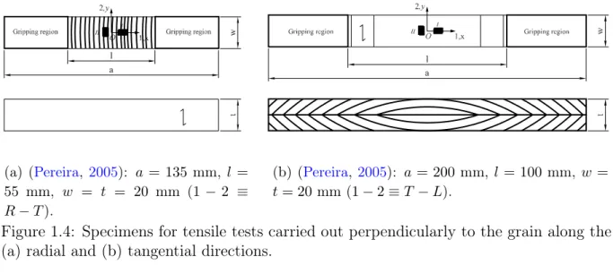
1.4 Specimens for tensile tests carried out perpendicularly to the grain along
the (a) radial and (b) tangential directions. . . 16
1.5 Schematic representation of specimens for compression testing. Parallel to
grain longitudinal compression (ASTM D143, 1994): l = 200 mm, w = t =
50 mm (1 − 2 ≡ L − R). . . 17
1.6 Off-axis tensile test: (a) schematic representation (l = 200 mm, w =
20 mm, t = 5 mm, α = 15◦); (b) rectangular and oblique end tabs. . . . 19
1.7 Schematic representations of: (a) the Iosipescu shear test; (b) the Iosipescu
fixture. . . 21
1.8 Schematic representations of: (a) the Arcan shear test (for clear wood specimen: l = 70 mm, w = 50 mm, t = 8 mm, d = 30 mm, r = 2 mm and
θ = 110◦); (b) the Arcan fixture. . . . 23
1.9 Schematic representations of the shear tests: (a) the in-plane shear test (Yoshihara and Matsumoto,2005); (b) the quasi-simple shear test (Naruse,
2003); (c) the square-plate twist test (Yoshihara and Sawamura, 2006). . . 25
1.10 Schematic representation of: (a) the 3 point bending test (for clear wood specimen: d ≥ 420 mm, L = {107, 129, 173, 400} mm, w = 20 mm, t = 20 mm and r = 15 mm); (b) the variable span method for the identification
of the longitudinal and shear moduli (β = R, T ). . . 26
1.11 Schematic representation of the four-point bending test (EN 408 (2002):
d = 380 mm, a = 120 mm, b = 120 mm, w = t = 20 mm, and r = 15 mm). 26
3.1 Schematic representation of the unnotched Iosipescu test. x − y is the
specimen coordinate system; 1 − 2 is the material coordinate system. . . . 56
3.2 (a) Schematic representation of the grid principle: (a) imaging system (b)
grid deformation. . . 57
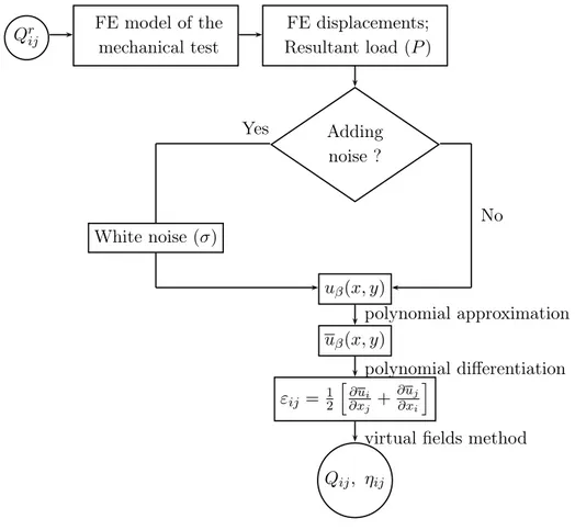
3.3 Image processing and identification flowchart. . . 59
3.4 Images of the: (a) crossed grid, I(x, y); (b) vertical lines grid, Ix(x, y); (c) horizontal lines grid, Iy(x, y). . . 60 3.5 Weighting matrix: (a) first iteration (3.5% of invalid pixels over the region
of interest); (b) second iteration (8.3% of invalid pixels over the region of interest). . . 64
3.6 Schema of the unnotched Iosipescu test illustrating the application of the virtual fields method. x − y and 1 − 2 are the specimen and material
coordinate systems, respectively. . . 65
4.1 Algorithm implemented in the validation of the material characterisation
approach (β = x, y, i, j = 1, 2, 6). . . 74
4.2 (a) Finite element model of the unnotched Iosipescu test, with L = 34 mm
(δ = 0.4 mm, FE size = 0.6 mm); (b) meshing refinement study – Qr
ij and
Qij are, respectively, the reference and identified stiffness parameters. . . . 75
4.3 (a) Variation of the sensitivity coefficients, ξij = ηij/Qij, with regard to the
gauge length L; (b) evaluation of the objective function φ(L). . . 78
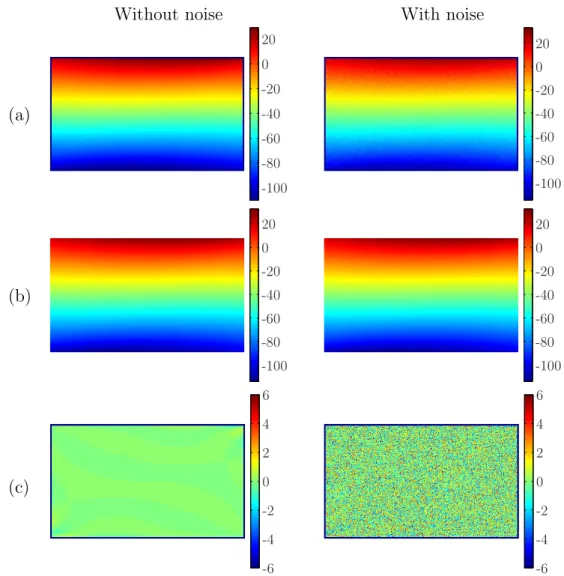
4.4 (a) Simulated, (b) approximated (7th-degree polynomial) and (c) residual
uxdisplacement component obtained for the 0◦specimen (without and with
adding a Gaussian white noise with σu = 2 µm) (unit: µm). . . 79
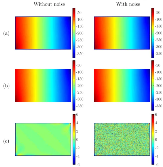
4.5 (a) Simulated, (b) approximated (7th-degree polynomial) and (c) residual
uy displacement component obtained for the 0◦specimen (without and with
adding a Gaussian white noise with σu = 2 µm) (unit: µm). . . 80
4.6 Evaluation of the residual (∆uβ, β = x, y) of the difference between
simu-lated (uβ) and approximated (uβ) displacement fields, with the increase of
the degree (d) of the fitting polynomial (unit: µm). . . 81
4.7 Typical strain fields (P = −261.8 N): (a) ε1, (b) ε2, (b) ε6, obtained for
the 0◦ specimen by differentiating (finite difference scheme) 2D polynomial
displacements with degrees (d) ranging from 5 to 11 (unit: ×10−3). . . . . 82
4.8 Relative differences of the (a) Q11, (b) Q22, (c) Q12 and (d) Q66
stiff-ness components, with regard to reference values, identified using
piece-wise virtual fields defined over a mesh of NX = {2, 3, . . . , 14} and NY =
{2, 3, . . . , 8} elements (using a 7th-degree polynomial displacement without
noise). . . 83
4.9 Graphical display of the mesh deformation corresponding to each optimised special virtual field used in the identification of: (a) Q11; (b) Q22; (c) Q12; (d) Q66. . . 84
4.10 Layered material model of the unnotched Iosipescu wood specimen. . . 86
4.11 (a) Simulated, (b) approximated (7th-degree polynomial) and (c) residual x and y displacement components obtained for the layered material model
(n = 10, wl= 0.4 and k = 2) (unit: µm). . . . 88
4.12 Strain field components (ε1, ε2 and ε6) of the layered material model (P =
−261.2 N): (a) obtained from numerical differentiation of the polynomial
displacement fields; (b) delivered directly from ANSYS (unit: ×10−3). . . . 89
4.13 Elastic constants: (a) E1, (b) E2, (c) ν12 and (d) G12, identified from
the layered material models by the virtual fields method (parametric data: (wl, k)). . . . 90 4.14 Algorithm used in the optimisation scheme of the configuration of the
un-notched Iosipescu specimen. . . 92
4.15 The cost function pattern as function of the L and θ design variables. . . . 94
4.16 Strain field maps (ε1, ε2 and ε6), along with their histograms plots, obtained
for the (L = 35 mm): (a) 0◦ configuration, (b) 30◦ configuration (unit:
×10−3). . . . 95
5.1 P. pinaster tree from where the specimens were manufactured. . . 98
5.2 Illustration of the steps in the grid transfer (p = 0.1 mm). . . 100
5.3 (a) Photo and (b) schematic of the mechanical set–up (WD (working
dis-tance) ∼ 450 mm). . . 102
5.4 (a) Grid image; (b) moiré effect used in the calibration of the optical system
magnification; (c) histogram of the grid image. . . 103
5.5 (a) Residual maps of the displacement typically obtained from experimental measurements; (b) Verification of the Gaussian distribution of the residual
values of the displacement (- · -: 2σ) (unit: µm).. . . 106
5.6 Variation of the stiffness parameters with respect to the degree of the fitting
polynomial for 0◦ (¥) and 45◦ (¤) specimens: (a) Q
11, (b) Q12, (c) Q22, (d) Q66. . . 108 5.7 (a) Measured, (b) approximated (7th-degree polynomial) and (c) residual
for ux and uy obtained for a 0◦ specimen (P = −139.4 N) (unit: µm). . . . 110
5.8 Typical (I) experimental and (II) numerical strain fields obtained for a 0◦
specimen (P = −139.4 N): (a) ε1, (b) ε2, (b) ε6. . . 111 5.9 Variation of the identified stiffness components with respect to the number
of elements used to set up the virtual mesh of the 0◦ specimen: (a) Q
11, (b) Q12, (c) Q22, (d) Q66. . . 111
5.10 Identified stiffness parameters as a function of the applied load for a 0◦ (¥)
and 45◦ (¤) specimens: (a) Q
5.11 (a) Measured, (b) approximated (7th-degree polynomial) and (c) residual
for ux and uy obtained for a 45◦ specimen (P = −143.0 N) (unit: µm). . . 116
5.12 Typical (I) experimental and (II) numerical strain fields obtained for a 45◦
specimen (P = −143.0 N): (a) ε1, (b) ε2, (b) ε6. . . 117 5.13 Variation of the identified stiffness components with regard to the number
of elements used to set up the virtual mesh of the 45◦ specimen: (a) Q
11, (b) Q12, (c) Q22, (d) Q66. . . 117
5.14 Typical (I) experimental and (II) numerical strain fields obtained for a 30◦
specimen (P = −176.5 N): (a) ε1, (b) ε2, (b) ε6. . . 120
5.15 Identified stiffness parameters as function of the applied load for a 30◦
specimen: (a) Q11, (b) Q22, (c) Q12, (d) Q66. . . 120 6.1 (a) Logs (1, 2, 3 and 4) of the P. pinaster tree from where specimens
were manufactured; (b) schematic representation of the specimen sampling
within the stem. . . 125
6.2 Curves of load versus cross-head displacement obtained at vertical location 1 for the radial positions : (a) r1; (b) r2; (c) r3; (d) r4; (e) average curves
(displacement rate of 1 mm/min). . . 127
6.3 Curves of load versus cross-head displacement obtained at vertical loca-tion 2 for the radial posiloca-tions: (a) r1; (b) r2; (c) r3; (d) average curves
(displacement rate of 1 mm/min). . . 128
6.4 Variation of the oven-dry density (ρ) at vertical locations 1 (¥) and 2 (¤)
with the radial positions. . . 128
6.5 Identified stiffness parameters at vertical location 1 as a function of the applied load: (a) Q22; (b) Q66. . . 131 6.6 Identified stiffness parameters at vertical location 2 as a function of the
applied load: (a) Q22; (b) Q66. . . 131
6.7 Stiffness values: (a) Q22; (b) Q66, identified at vertical position 1 for the
radial positions r1, r2, r3 and r4 (unit: ρ - g.cm−3; Qij - GPa). . . 134 6.8 Stiffness values: (a) Q22; (b) Q66, identified at vertical position 2 the radial
positions r1, r2 and r3 (unit: ρ - g.cm−3; Qij - GPa). . . 135
6.9 Variation of the stiffness parameters: (a) Q22; (b) Q66, identified at the two
vertical locations 1 (¥) and 2 (¤) as a function of the radial position (r/R).136
6.10 Comparison of the stiffness parameters: (a) Q22; (b) Q66, identified at the
two vertical locations 1 (¥) and 2 (¤) at the outmost radial position, r4
2.1 Optical methods in experimental mechanics. . . 36
2.2 Some heterogeneous mechanical tests for the identification of constitutive
parameters. . . 53
4.1 Reference elastic engineering properties of P. pinaster wood used in the
finite element analyses (Pereira, 2005; Xavier et al., 2004) (1 − 2 ≡ L − R). 75
4.2 Stiffness parameters identified by the virtual fields method (with a mesh of 8(x)×4(y) elements) from the finite element strains, without (Ident. 1) and
with (Ident. 2) noise (σε= 10−4, 30 iterations), and from the finite element
displacements, without (Ident. 3) and with (Ident. 4) noise (σu = 2 µm, 30
iterations) (unit: GPa) (1 − 2 ≡ L − R). . . 85
4.3 Earlywood and latewood elastic engineering properties used in the finite
element analyses (k = 2, wl= 0.4) (1 − 2 ≡ L − R). . . . 87
4.4 Identification of homogenised elastic engineering properties of the layered material model of the unnotched Iosipescu wood specimen by the virtual fields method: (1) directly from the finite element strain fields without noise (Ident. 1); (2) from the finite element displacement maps without noise (Ident. 2). Ident. 3: identification results obtained from the homogeneous
material model (from Ident. 1 in Table 4.2) (1 − 2 ≡ L − R). . . 91
5.1 Reference stiffness values of P. pinaster wood identified using standard
tests (moisture content of about 11%) (Pereira, 2005; Xavier et al., 2004)
(1 − 2 ≡ L − R). . . 112
5.2 Stiffness properties of P. pinaster wood identified by the virtual fields
method (virtual mesh of 8(x)×4(y) elements) from the 0◦ specimens
(mois-ture content about 9–10%) (1 − 2 ≡ L − R). . . 113
5.3 Stiffness properties of P. pinaster wood identified by the virtual fields
method (virtual mesh of 5(x) × 3(y) elements) from the 45◦ specimens
(moisture content about 9–10%) (1 − 2 ≡ L − R). . . 118
6.1 Comparison of mean values between the different radial positions at vertical location 1 by the Student’s t-test of equality of means of two samples at a
95% of confidence level (1 − 2 ≡ L − R). . . 132
6.2 Comparison of mean values between the different radial positions at vertical location 2 by the Student’s t-test of equality of means of two samples at a
Wood is a natural composite material formed by trees. Since trees are a valuable resource on earth, historically, wood has always played an important role as a material (e.g., in construction). In more recent decades, manufacturing developments have led to new engineering products based on raw wood material – such as glued laminated timber, structural plywood, oriented strand board (OSB), laminated veneer lumber (LVL) and wood I-joists – specifically designed to fit structural requirements (Williamson, 2002). Both solid wood and its derivative products constitute nowadays important engineering materials owing to the following reasons (STEP, 1996): (1) trees are produced by a free source of energy (the sun) and they are renewable and recyclable; (2) there are important forestal resources on earth; (3) the sylviculture and wood transformation have a relatively low cost; (4) the wood material has good stiffness to weight and strength to weight ratios. Nevertheless, for the efficient utilisation of wood in engineering applications, the material parameters governing relevant constitutive equations (e.g., the stiffness parameters in the linear elastic anisotropic model) as well as other properties such as strength values, must be properly characterised for each species (ASTM D143,1994;Bodig and Goodman,
1973).
As a rough approximation, the stem of a tree can be conceptualised as a cylindrical orthotropic material (Guitard, 1987; Smith et al., 2003). Three planes of symmetry are locally defined by the longitudinal (L, 1), radial (R, 2) and tangential (T, 3) principal di-rections of the longitudinal wood cells (tracheids in softwood). The mechanical properties of wood are usually identified in this material coordinate system; properties along differ-ent directions can be determined from standard transformation equations afterwards. The mechanical behaviour of wood can be analysed hierarchically over a spectrum of length scales. At the macroscopic scale, clear wood (i.e., defects-free and straight-grained wood) is normally assumed as a solid (continuous) and homogeneous material. Different consti-tutive equations have been proposed in the literature for clear wood modelling, each of them with a specific domain of validity. Neglecting any deformation generated by hygro-thermal effects, the constitutive equations generally accepted are the linear elastic and viscoelastic models (Dinwoodie,2000;Guitard,1987; Holmberg et al.,1999;Kollman and Côté Jr., 1984; Smith et al., 2003). Wood seems to be more accurately described by the viscoelastic theory since experimental observations have revealed a strain-rate dependence
on its mechanical response. However, for most practical applications, the time dependent deformation may be neglected and wood can simply be considered as a linear elastic solid. This theory assumes relatively low levels of stress (below the elastic limit), applied over a short period of time (a few minutes) and at room temperature. The elastic parameters governing the linear elastic constitutive equation have been recognised as fundamental data in the following applications: (1) for the comparison of properties among trees and species (ASTM D143, 1994; Dinwoodie, 2000); (2) for understanding the effects on wood mechanical properties of factors such as density, moisture content, geographical origin and positions within the stem (ASTM D143, 1994; Dinwoodie, 2000; Guitard, 1987;Kollman and Côté Jr., 1984; Machado and Cruz, 2005); (3) for the numerical and experimental analyses of the deformation of structural wood members (Bodig and Goodman, 1973;
Sliker, 1985); (4) for capturing genetic breeding opportunities and also for improving the stiffness properties of juvenile wood in fast grown conifers (Lindström et al., 2002).
Furthermore, one major advantage of the assumption of linear elasticity is that quasi-static mechanical tests can be carried out for the characterisation of the elastic properties of wood. However, because of the orthotropy of the wood structure, several independent tests are usually required (Guitard,1987). Such methods rely on simple loading conditions (tension, compression, shear or bending) for which a simple state of stress is assumed over a representative volume element of the material at the scale of analysis. In these cases, an analytical (closed-form) solution can be derived, directly linking the load and strain mea-surements to the unknown material parameters. Owing to anisotropy and heterogeneity, the requirement for improved mechanical test methods has soon emerged (Jones, 1999;
Tarnopol’skii and Kulakov, 1998). In this field of research, several mechanical tests have been designed and improved for this type of material (e.g., the off-axis tensile test and the Iosipescu shear test). Nevertheless, some drawbacks have been pointed out to these methods, namely, the practical difficulty of generating a uniform stress/strain field across the region of interest because of both end and edge effects (Grédiac, 1996; Tarnopol’skii and Kulakov,1998).
For the identification of representative parameters of a given species of wood, several specimens, cut at random locations within the stem and from different trees, need to be tested in order to account for the inherent structural variability of wood (Bodig and Goodman, 1973). Hence, owing to the anisotropy and variability of wood, it can be concluded that a significant amount of tests are required, which is quite expensive and time consuming. To simplify this procedure, an approach has been proposed since the early work of Bodig and Goodman(1973). Basically, it consists in deriving relationships among wood properties. Since the longitudinal elastic modulus is known for most species, this parameter has been often taken as the independent variable (Bodig and Goodman,
1973; Green et al., 1999; Sliker, 1985, 1988; Sliker and Yu, 1993). The prediction of the elastic parameters from physical properties such as the density has also been the object of
research in several studies (Bodig and Goodman,1973;Gibson and Ashby,1997;Guitard,
1987;Sliker and Yu,1993;Walton and Armstrong,1986). An alternative approach is used in this work.
Thanks to the advent of full-field optical methods, which provide the measurement of kinematic quantities (e.g., displacement, slope, strain or curvature) over a whole region of interest, a new perspective on mechanical testing for material characterisation has been progressively introduced (Grédiac, 1996, 2004). The basic idea is that a single specimen can be loaded in such a way that several parameters are simultaneously involved in its mechanical response, yielding complex and heterogeneous stress/strain fields. Providing that these fields are measured by a suitable optical method, the whole set of active pa-rameters can be determined afterwards by an appropriate identification strategy. This approach seems to be particularly convenient for a material like wood. Indeed, it has been already applied to wood or wood based products by a few authors (Cárdenas-García et al.,2005;Foudjet et al.,1982;Jernkvist and Thuvander,2001;Le Magorou et al.,2002;
Rouger, 1988).
The aim of this work is to apply this inverse identification approach to the charac-terisation of the longitudinal-radial, (L, R) ≡ (1, 2), stiffness parameters (Q11, Q22, Q12
et Q66) of maritime pine (Pinus pinaster Ait.) wood. Particularly, the proposed
pro-cedure is based on the application of the virtual fields method (VFM) to a rectangular specimen loaded in the Iosipescu fixture. Displacement fields are measured by the opti-cal grid method. Eventually, a contribution to the spatial variability of the LR stiffness parameters within the stem is proposed.
This report consists of six chapters. In chapter 1, the linear elastic behaviour of wood is reviewed, with emphasis being placed on the standard mechanical tests usually employed for its characterisation. The full-field optical methods most commonly used in experimental mechanics and their interest to wood mechanics are outlined in Chapter 2, along with a presentation of statistically undetermined tests and the general principle of the VFM. Chapter 3 presents the inverse identification approach proposed in this work. The numerical and experimental validation of this approach are studied in Chapters 4 and 5, respectively. Chapter 6 describes the application of the proposed methodology in accessing the spatial variability of the stiffness parameters within the stem. Finally, the general conclusions and some directions for future work are given.
The linear elastic behaviour of clear
wood: a review
1.1
Hierarchical structure and modelling of wood
1.1.1
Introduction
Trees can be classified, into two main groups, according to their anatomy: softwoods (Gymnospermae) and hardwoods (Angiospermae). Although the nature and composition of wood is basically the same for all trees, this classification is justified because the types of cells, their proportions and arrangements greatly differ from one species to another. As maritime pine wood (Pinus pinaster Ait.) was used as tested material in this work, this section will focus specifically on softwood species.
A tree is a vascular woody plant which contains three main parts: the root system, the stem and the crown system. Only the stem of the tree will be considered. The wood within the stem has a heterogeneous structure which can be observed hierarchically over a spectrum of length scales as illustrated in Figure 1.1.
In understanding the mechanical behaviour of wood it is important to be acquainted with its morphology. The main features of the wood structure are reviewed below, based on the following references: Dinwoodie (2000); Guitard (1987); Kollman and Côté Jr.
(1984); Smith et al. (2003).
From a mechanical point of view, different models along with test methods are usually applied along the hierarchical scales. At each relevant scale of observation, the basic assumptions on which wood modelling relies on are also summarised in this section.
1.1.2
Massive scale: structural wood
At the structural scale (> 1 m), several growth features can be distinguished within the stem such as juvenile and mature wood, knots, reaction wood and spiral grain
(Fig-Massive scale
(< 1 m) =⇒ (a)
knots Reaction wood Spiral grain
Macro scale (0.1-1 m) =⇒ (b) Clear wood Meso scale (1-10 mm) =⇒ (c) Micro scale (10-100 µm) =⇒ (d)
Figure 1.1: Hierarchical scales of wood.
ure1.1(a)). Juvenile wood is a layer of wood surrounding the pith typically formed within the first 5-20 annual growth rings. This wood consists of cells formed by juvenile cambium and exists in all trees. Compared with mature wood, which is formed later in the growing process, juvenile wood is characterised by short cells with large diameter lumen (hollow of the cell), thin cell walls, and usually has more knots. Furthermore, the physical and mechanical properties of juvenile wood are spatially less uniform than the ones of mature wood. Knots (Figure 1.1(a)) are sections of the tree branches that are embedded in the wood of the stem. They create localised disturbances in the orientation of the longitu-dinal wood cells, resulting in wood structure, and therefore wood properties, variations. Reaction wood (Figure 1.1(a)) is another component of the tree, associated with the
ec-centrical location of the pith and abnormal growth rings formed by trees as a reaction to adverse external forces (e.g., the wind). In softwood, the growth rings are abnormally wide on the underside of an inclined stem, leading to what is called compression wood. Key disadvantages of reaction wood, compared to normal wood, are the reduction of the strength and the augmentation of shrinkage along the grain. Another important feature about the wood architecture is the alignment of the longitudinal wood cells with regard to the long axis of the stem, called spiral grain (Figure1.1(a)). The grain is usually arranged either in a right- or left- handed helical or spiral pattern around the stem. This pattern usually changes during the growing of the tree. The local orientation of the grain can be defined by the radial (α) and tangential (β) angles formed with regard to the longitudi-nal direction of the stem (Figure 1.1(a)). The spiral grain can lead to the reduction of the mechanical properties of wood and the enhancement of its tendency to twist during drying.
Conceptually, the wood of a tree can be modelled as a cylindrical orthotropic material having three planes of symmetry (sections 1, 2 and 3 in Figure 1.2) along its longitu-dinal (L, 1), radial (R, 2) and tangential (T, 3) directions. At the structural scale and for engineering design purposes, the cylindrical orthotropy of wood is usually turned into transverse isotropy, i.e., the mechanical properties of wood are assumed identical across the radial-tangential (R −T ) plane (ASTM D143,1994;EN 408,2002;STEP,1996). This assumption is based on the observation that the anisotropy ratio ER/ET is usually close
to unity – e.g., ER/ET = 1.9 for P. pinaster wood (Pereira,2005). The properties of wood
along the transversal cross-section are usually referred in the literature as perpendicular to grain, whereas along the longitudinal direction they are referred to as parallel to grain.
1.1.3
Macro scale: clear wood
The features of wood at the macroscopic level (0.1-1 m) can be observed by considering the cross-section (1), the radial-section (2), and the tangential-section (3) of the stem (Figure 1.2). In the cross-section the following layers can be distinguished: pith (4), heartwood (5), sapwood (6), cambium (8) and bark (9) (Figure 1.2). The pith consists of soft spongy cells with low strength and durability, located in the centre part of the stem. Typically its diameter is of a few millimeters. Surrounding the pith there are the heartwood and sapwood layers, which are the inward and outward parts of the stem, respectively. The heartwood is typically darker than sapwood. The width and colour of these layers can vary significantly between species. The cells in the heartwood are dead and they contribute mostly to the structural support of the tree. Also, this region accumulates the function of storage of the excess of nutrients, that are metabolised into extractives such as resin and tannins. Sapwood is used by the tree for conducting water and nutrients, necessary for its growing process. After these layers, which constitute the
Figure 1.2: Macrostructure features of the softwood stem: (1) cross-section; (2) radial-section; (3) tangential-radial-section; (4) pith; (5) heartwood; (6) sapwood; (7) growth ring; (8) cambium; (9) bark; (10) rays (L– longitudinal, R–radial and T –tangential).
wood material of the stem or xylem, follows the vascular cambium, which is a thin layer located just beneath the bark where the formation of new cells takes place. The cells of the cambium divide, forming wood (xylem) to the inside and bark (phloem) to the outside. Thus, the stem of the tree increases radially and longitudinally. Finally, the bark is the outermost layer of the stem whose function is the protection of the tree from its surrounding environment.
For species growing in temperate climates, alternately concentric regions are visible (7), corresponding to the annual growth increments of wood (Figure 1.2). The wood rays (10), consisting of parenchyma cells, can be observed in the radial section and they represent only a small percentage (5-10%) of the entire wood in the stem (Figure 1.2). They are organised in tissues disposed from the pith to the bark, and their main function is the storage of nutrients. These cells are perpendicular to the longitudinal ones (tracheids), and give some strength and stiffness to wood in the radial direction.
At this scale, wood is called clear wood because it is assumed free from structural defects such as knots and gross grain deviation. A sample of clear wood is usually assumed to be homogeneous, i.e., an elementary representative volume of material with uniform mechanical properties. In addition, as the characteristic dimensions of the sample are much larger than the microscopic cellular structure of wood (a few tenths of a micrometre), the assumption of a continuum medium is justified. The wood cells formed in the growing process of a tree are roughly arranged longitudinally in concentric circles within the stem. If a sample of wood is cut at a sufficient distance from the pith (i.e., in the outward part of the stem), such as the curvature of the growth rings can be neglected, wood may be simply modelled assuming rhombic orthotropy. Locally at each material point within the stem, three principal material directions of wood are defined: the longitudinal direction (L, 1) along the grain; the radial direction (R, 2) perpendicular to the longitudinal cells and parallel to the rays; and the tangential direction (T, 3) tangent to the growth ring and
perpendicular to L and R (Figure 1.2). These directions define the material coordinate system.
1.1.4
Meso scale: growth ring
At this scale of magnification (1-10 mm) the cellular structure of wood can be observed (Figure1.1(c)). It consists of an aggregate of cells, often with an hexagonal shape, aligned with the direction of the stem. At this level, an individual annual growth ring can be assumed consisting of two principal layers called, respectively, earlywood (springwood) and latewood (summerwood) (Figure 1.1(c)). The early and late woods are formed at the beginning and at the end of the growing season (spring) respectively. The transition from earlywood to latewood occurs gradually (a transition zone may be distinguished), as opposed to the latewood to earlywood one which is rather abrupt. The cells in the earlywood are characterised by thin walls and large diameters, whilst it is the converse for the latewood, where the cells are smaller in diameter and have thick walls. The growth rate of the tree is different throughout the years, resulting in the radial variation of the width of the annual rings within the stem. As a typical pattern, founded for instance in P. pinaster wood, the annual rings are wider in the centre and thinner at the periphery; besides, the width of the latewood layer tends to be constant. Furthermore, although the cross-section of the stem is roughly circular, the annual rings do not necessarily develop uniformly in all the radial directions due to effects such as the direction of sunlight, the shade and the topography of the growth site. This can induce, for instance, the formation of reaction wood (§ 1.1.2).
At the meso scale, wood is usually analysed and modelled as a cellular solid material. Honeycomb models of the aggregate of wood cells (unit cell method) have been proposed for estimating the stiffness of the cellular wood material from the cell geometry, cell wall properties and applied beam theory.
1.1.5
Micro scale: cell level
The wood cell wall (10-100 µm) is a layered structure consisting of middle lamella (M), primary wall (P) and secondary wall (S) (Figure 1.1(d)). Each layer consists of an amor-phous matrix made up of hemicelluloses and lignin, reinforced by highly ordered bundles of cellulose chains called microfibrils. The orientation of the microfibrils, with regard to the long cell axis, is called the microfibril angle (MFA). Cells are joined together by the middle lamella. The primary wall is usually very thin, about 0.1 µm, and has randomly distributed microfibrils. Their distribution is more organised within the secondary wall. In both S1 and S3 secondary-wall layers, the microfibrils are oriented almost perpendicu-lar to the cell axis. However, in the S2 layer, the thickest of the three (about 80% of the cell wall thickness), the microfibrils form a right-handed spiral and are nearly oriented
parallel to the cell axis.
At this scale, wood can be modelled as a natural fibre-reinforced composite laminated material. The lay-up of the cellulose microfibrils within the cell wall (i.e., the variation of the MFA across the cell wall thickness, especially in the S2 secondary layer) as well as the elongated geometry of the cell (the length of the cell is about 100-fold greater than the dimensions of its cross-section), play an important role in the stiffness and anisotropy of the wood cell wall.
1.1.6
Conclusions
Trees can be distinguished by their anatomical structure into softwood and hardwood species. Maritime pine wood (Pinus pinaster Ait.), which belongs to softwoods species, was selected as the material for this work. P. pinaster wood is an important species in Southern Europe. In Portugal, it represents about 23% (almost 1 hectare) of the total forest area of the country and 88% of the volume of raw material consumed in wood-based industries (e.g., sawmill, plywood, particle board, pulp and paper) (DGF, 2007).
The structure and the mechanical behaviour of wood can be analysed hierarchically at several length scales. At each level, different assumptions and models are usually assumed. In this work, wood will be analysed at the macroscopic scale. At this scale, wood is modelled as a continuous (solid) and homogeneous material, with three plane of orthotropic symmetry defined by the longitudinal (L), radial (R) and tangential (T ) directions of the wood cells (tracheids).
1.2
Constitutive behaviour of clear wood
1.2.1
Introduction
Owing to the biological nature of wood, its deformation process can be quite complex. At low levels of stresses, experimental observations have suggested that wood can be modelled as an anisotropic, viscoelastic and hygroscopic material. The anisotropy nature of wood means that the mechanical properties at a given material point are directionally dependent (Guitard,1987, p. 57). The viscoelasticity of wood implies that its mechanical properties are sensitive to strain rate (Widehammar, 2006). In the hygroscopic domain, defined between the anhydrous and cell wall saturation states (§ 1.4.3.1), the ability of wood to exchange humidity with its surrounding environment can be responsible for an additional free shrinkage or swelling deformation (Badel and Perré, 2001). Moreover, when wood is simultaneously subjected to loading and moisture content changes below the fiber saturation point (§ 1.4.3.1), the mechano-sorptive effect may be observed as an additional deformation (Muszyński et al., 2005).
Consequently, it can be concluded that the constitutive modelling of all different con-tributions on the mechanical behaviour of wood can be quite complex. Particularly, from the experimental point of view, the parameter identification can be a rather difficult task (Muszyński, 2006; Muszyński et al., 2005). Based on the fact that the constitutive be-haviour of wood depends on the actual application, i.e., on the type and duration of load and on environmental effects (moisture and temperature variations) to be considered, hy-pothesis and assumptions are usually postulated, restricting the analyses to particular mechanical responses. In the simplest case, involving low levels of stress (below the elas-tic limit), short periods of time (a few minutes) and minor variations of moisture content and temperature (absence of hygro-thermal environment effects), it should be sufficient to simply assume wood as a linear elastic anisotropic material (Dinwoodie,2000, p. 94). In other cases, however, such as in wood drying, it is necessary to include mechano-sorptive effects and creep in the model (Holmberg et al., 1999). Besides, under conditions of very heavy loading, such as in defibration or wood machining, account must be taken of large deformations and fracture (Holmberg et al.,1999;Reiterer and Stanzl-Tschegg, 2001).
In this work, anisotropic linear elastic behaviour is assumed. A brief summary of linear orthotropic elasticity is presented in the following subsection.
1.2.2
Anisotropic linear elastic constitutive behaviour
1.2.2.1 Constitutive equations for an orthotropic materialAt a given material point, the linear elastic constitutive law is defined by a linear relationship between the stress (σ) and strain (ε) tensors:
σij = Cijklεkl (i, j, k, l = 1, 2, 3) (1.1)
where Cijklis the fourth order stiffness tensor whose components are the elastic parameters
of the material. Using Voigt notation and assuming orthotropy, Eq. (1.1) can be written in the axes of orthotropy (O, e1, e2, e3) as:
σ1 σ2 σ3 σ4 σ5 σ6 = C11 C12 C13 0 0 0 C21 C22 C23 0 0 0 C31 C32 C33 0 0 0 0 0 0 C44 0 0 0 0 0 0 C55 0 0 0 0 0 0 C66 ε1 ε2 ε3 ε4 ε5 ε6 (1.2a)
or in compact matrix notation
where {σ} and {ε} are, respectively, the stress and strain pseudo-vectors and [C] the stiffness matrix, which is symmetric and positive definite. The complete identification of the nine independent stiffness components of matrix [C] requires classically several independent tests: three uniaxial tensile/compression tests along the material principal directions and three shear tests along the planes of symmetry.
1.2.2.2 Plane stress assumption
An important issue in the experimental characterisation of materials is the plane stress assumption. This approach is verified when the shape of the test specimen is reduced to a plane. In this case, only the in-plane stress components are significant and they are assumed to be constant across the thickness. Accordingly and considering the 1 − 2 plane of symmetry, Eq. (1.2) can be reduced to (σ3 = σ4 = σ5 = 0):
σ1 σ2 σ6 = Q11 Q12 0 Q12 Q22 0 0 0 Q66 ε1 ε2 ε6 (1.3a) or {σ} = [Q]{ε} (1.3b)
where [Q] is the reduced stiffness matrix, which can be determined directly from [C] (Eq. 1.2) according to:
Qij = Cij −
Ci3Cj3
C33
(i, j = 1, 2, 6). (1.3c)
The constitutive equations given in (Eq. 1.3a) can be written for an arbitrary orienta-tion between the specimen (x − y) and material (1 − 2) coordinate systems using classical formulas of matrix transformation (Jones, 1999, §2.6).
1.2.2.3 Engineering constants
The stiffness matrix in the constitutive equations (1.3) is determined experimentally from appropriate mechanical test methods. Historically, in the interpretation of these tests engineering constants have been introduced, linked directly to the load and strain measurements. The stiffness and engineering constants can be related by the following equalities (Jones, 1999, p. 72):