The Behavior of the Maximum Likelihood Estimator of Dynamic Panel Data Sample Selection Models

Texte intégral

(1)2007s-06. The Behavior of the Maximum Likelihood Estimator of Dynamic Panel Data Sample Selection Models Wladimir Raymond, Pierre Mohnen, Franz Palm, Sybrand Schim van der Loeff. Série Scientifique Scientific Series. Montréal Mars/March 2007. © 2007 Wladimir Raymond, Pierre Mohnen, Franz Palm, Sybrand Schim van der Loeff. Tous droits réservés. All rights reserved. Reproduction partielle permise avec citation du document source, incluant la notice ©. Short sections may be quoted without explicit permission, if full credit, including © notice, is given to the source..

(2) CIRANO Le CIRANO est un organisme sans but lucratif constitué en vertu de la Loi des compagnies du Québec. Le financement de son infrastructure et de ses activités de recherche provient des cotisations de ses organisations-membres, d’une subvention d’infrastructure du Ministère du Développement économique et régional et de la Recherche, de même que des subventions et mandats obtenus par ses équipes de recherche. CIRANO is a private non-profit organization incorporated under the Québec Companies Act. Its infrastructure and research activities are funded through fees paid by member organizations, an infrastructure grant from the Ministère du Développement économique et régional et de la Recherche, and grants and research mandates obtained by its research teams. Les partenaires du CIRANO Partenaire majeur Ministère du Développement économique, de l’Innovation et de l’Exportation Partenaires corporatifs Alcan inc. Banque de développement du Canada Banque du Canada Banque Laurentienne du Canada Banque Nationale du Canada Banque Royale du Canada Banque Scotia Bell Canada BMO Groupe financier Bourse de Montréal Caisse de dépôt et placement du Québec DMR Conseil Fédération des caisses Desjardins du Québec Gaz de France Gaz Métro Hydro-Québec Industrie Canada Investissements PSP Ministère des Finances du Québec Raymond Chabot Grant Thornton State Street Global Advisors Transat A.T. Ville de Montréal Partenaires universitaires École Polytechnique de Montréal HEC Montréal McGill University Université Concordia Université de Montréal Université de Sherbrooke Université du Québec Université du Québec à Montréal Université Laval Le CIRANO collabore avec de nombreux centres et chaires de recherche universitaires dont on peut consulter la liste sur son site web. Les cahiers de la série scientifique (CS) visent à rendre accessibles des résultats de recherche effectuée au CIRANO afin de susciter échanges et commentaires. Ces cahiers sont écrits dans le style des publications scientifiques. Les idées et les opinions émises sont sous l’unique responsabilité des auteurs et ne représentent pas nécessairement les positions du CIRANO ou de ses partenaires. This paper presents research carried out at CIRANO and aims at encouraging discussion and comment. The observations and viewpoints expressed are the sole responsibility of the authors. They do not necessarily represent positions of CIRANO or its partners.. ISSN 1198-8177. Partenaire financier.

(3) The Behavior of the Maximum Likelihood Estimator of Dynamic Panel Data Sample Selection Models* Wladimir Raymond†, Pierre Mohnen‡, Franz Palm§, Sybrand Schim van der Loeff ** Résumé / Abstract Cette étude propose une façon d’utiliser l’estimateur du maximum de vraisemblance pour des données panel et des modèles dynamiques de type tobit 2 ou tobit 3. La fonction de vraisemblance inclut une intégrale double qui est évaluée en utilisant une quadrature GaussHermite à deux étapes. Une étude de Monte Carlo montre que la quadrature donne de bons résultats dans un échantillon fini même avec uniquement deux points d’évaluation. Si on ignore les effets individuels ou la dépendance entre ceux-ci et les conditions initiales, on obtient une estimation biaisée vers le haut des coefficients des variables endogènes retardées. Une application à l’étude des innovations de produit radicales et incrémentales avec des données panel d’entreprises néerlandaises illustre la méthode proposée. Mots clés : données panel, maximum de vraisemblance, modéles dynamiques avec sélection. This paper proposes a method to implement maximum likelihood estimation of the dynamic panel data type 2 and 3 tobit models. The likelihood function involves a two-dimensional indefinite integral evaluated using “two-step” Gauss-Hermite quadrature. A Monte Carlo study shows that the quadrature works well infinite sample for a number of evaluation points as small as two. Incorrectly ignoring the individual effects, or the dependence between the initial conditions and the individual effects results in an overestimation of the coefficients of the lagged dependent variables. An application to incremental and radical product innovations by Dutch business firms illustrates the method. Keywords: panel data, maximum likelihood estimator, dynamic models, sample selection. *. Acknowledgements: The empirical part of this study has been carried out at the Centre for Research of Economic Microdata at Statistics Netherlands. The authors wish to thank Statistics Netherlands, and in particular Bert Diederen, for helping them in accessing and using the Micronoom data set. They wish to thank François Laisney for his helpful comments. The first author acknowledges the financial support from METEOR. † University of Maastricht, w.raymond@ke.unimaas.nl ‡ University of Maastricht, MERIT and CIRANO, p.mohnen@merit.unimaas.nl § University of Maastricht and CESifo fellow, Universiteit Maastricht, P.O. Box 616 6200 MD Maastricht, The Netherlands; Tel: +31 43 388 3833; Fax: +31 43 388 4874; f.palm@ke.unimaas.nl ** University of Maastricht, s.loe®@ke.unimaas.nl.

(4) 1. Introduction. The ongoing development of the relevant econometric methodology for panel data has increased the choice for the applied researcher as to which model to choose in any given situation. Whereas this choice should be driven by the question which underlying assumptions are appropriate in the case at hand, optimality properties of the estimators are typically known only for large sample sizes. In order to have some guidance in the choice process it is important to know the implications, in terms of ease of computation, finite sample properties and the robustness to deviations of the assumptions, of employing a particular method. In this paper the behavior of the maximum likelihood (ML) estimator is investigated by means of Monte Carlo simulations in a general model that encompasses a wide set of models that have been considered in the literature. The generic form of the model consists of a regression equation, henceforth referred to as the equation of interest, and a selection equation. Both equations contain a lagged dependent variable and unobserved individual effects possibly correlated with the explanatory variables. The selection rule may be of the binary type or of the censoring type.1 In terms of the Amemiya (1984) typology, the models considered in this paper are the dynamic panel data extensions of the type 2 and type 3 tobit models.2 Variants of these types of models have been widely used, mostly in labor economics but also in other areas, but only in a static or “partial” dynamic framework (see Table 1). This study contributes to the existing literature in a number of ways. Firstly, a practical method is provided to implement maximum likelihood estimation of the parameters of a panel sample selection model in which random individual effects and the lagged dependent variable are included in the equation of interest as well as in the selection equation. The selection rule may be either of the binary or of the censoring type.3 To handle the initial conditions problem, Wooldridge’s (2005) solution to this problem in single equation dynamic nonlinear panel data models is extended to models containing more than one equation. Gaussian quadrature is used to evaluate the resulting two-dimensional indefinite integral. Secondly, the paper reports on a Monte Carlo investigation into the behavior in finite samples of the proposed method. It is shown that using Wooldridge’s solution to deal with the dependence between the initial conditions and the individual effects is successful in recovering the parameters of a process that generates the data according to a stationary process. For the likelihood functions generated in the Monte Carlo 1 Following the literature the term censoring model will be used throughout the paper although it would, in line with Wooldridge (2005), be preferable to speak of corner solution models since the lagged dependent variable considered in this paper is the observed - rather than the latent - variable. 2 The type 3 tobit differs from the type 2 tobit in that the selection into the sample is made through a censored (partially continuous) variable instead of a binary variable. The former model uses more information to estimate the equation of interest than the latter. Hence, we should expect the estimation of the equation of interest to be more accurate in the former model than in the latter. 3 These are the types of selection rule that are mostly considered in the literature (see Table 1). Other types of selection rule are ordered, multinomial, and those based on multiple indices (Vella, 1998).. 2.

(5) experiments, Gaussian quadrature, implemented as two successive Gauss-Hermite approximations, works well for a number of evaluation points as small as two.4 Evidently, when using real data more than two evaluation points may be necessary to attain the required numerical accuracy. Nevertheless, the Monte Carlo results indicate that ML estimation of the parameters in a randomeffects dynamic sample selection model is feasible and could conceivably be incorporated as a command in a general use software package such as Stata. Thirdly, the sensitivity of the ML estimator to misspecification is also investigated. It is shown that incorrectly ignoring the individual effects, or the dependence between the initial conditions and the individual effects results in an overestimation of the coefficients of the lagged dependent variable in both equations. Fourthly, the paper deals with the estimation of type 2 and type 3 tobit in a “full” dynamic framework, and provides for the first time an application of the dynamic type 3 tobit to the economics of innovation. The remainder of the paper is organized as follows. We discuss the most cited studies on panel data sample selection models in Section 2. Section 3 describes the model and Section 4 describes its maximum likelihood estimation. The small sample behavior of the estimator is studied in a Monte Carlo study in Section 5, an application is provided in Section 6, and Section 7 concludes. The Gauss-Hermite quadrature is explained in Appendix A.. 2. Literature. Most of the studies on panel data sample selection models are of the type 2 or type 3 tobit (see Table 1), which are estimated by ML or two-step least squares (Heckman, 1979), or by variants of the two-step Heckman type estimator. For instance, Hausman and Wise (1979) describe a two-period model of attrition and estimate by ML the impact of attrition on earnings. Attrition is defined as the inability to observe the dependent variable of the equation of interest in the second period.5 Ridder (1990) generalizes the model of Hausman and Wise to allow for more than two periods and attrition to occur also in the first period. Hence Ridder’s model can be used as a standard attrition or sample selection model. Nijman and Verbeek (1992) apply this model to study the effect of nonresponse on Dutch households’ consumption. Verbeek (1990) assumes random and fixed individual effects in the selection and regression equations respectively, and estimates by ML a transformed model with a selection equation written in levels and a within-transformed equation of interest. Verbeek’s 4 The use of Gauss-Hermite quadrature, instead of simulated likelihood, is motivated by the finding of Guilkey and Murphy (1993) that, for the same accuracy, the former method is 5 times as fast as the latter (see also Greene, 2004b). 5 Attrition in the first period is usually referred to as sample selection.. 3.

(6) model is criticized by Zabel (1992) who considers random individual effects correlated with the explanatory variables in both the selection equation and the equation of interest and estimates the resulting model by ML. All these studies are of limited use to the applied researcher who wants to implement the ML estimator as they present only the general expression of the likelihood function which involves a multiple integral that is yet to be calculated. Our study makes a step in this direction. The two-step Heckman type estimator consists, in a first step, in estimating the selection equation and constructing an estimate of a selection correction term that is included as a regressor in the equation of interest which, in a second step, is estimated using ordinary least squares (OLS) regression. Wooldridge (1995) estimates an augmented equation of interest written in levels by pooled OLS where estimates of the selection correction terms are obtained, in a first step, using a probit model for each period. Kyriazidou (1997) and Honoré and Kyriazidou (2000) propose to estimate, by kernel-weighted least squares, a pairwise differenced equation of interest for individuals that are selected into the sample and have “the same” selection equation index in two different periods. Under a conditional exchangeability assumption, the sample selection is time-invariant for such individuals so that differencing the equation of interest over time wipes out, not only the individual effects, but also the sample selection effect. In order to construct the kernel weights, the parameters of the selection equation are estimated, in a first step, using conditional logit or smoothed conditional maximum score. Rochina-Barrachina (1999) applies OLS to a pairwise differenced equation of interest augmented with two selection correction terms for individuals that are selected into the sample in two different periods. Estimates of these selection correction terms are obtained, in a first step, using a bivariate probit for each combination of time periods. The studies cited so far consider sample selection models with a binary selection rule (type 2 tobit). Heckman and MaCurdy (1980) estimate by ML a fixed-effects type 3 tobit and apply it to a wage equation with a labor supply (the number of hours worked) equation as the selection equation. Ai and Chen (1992) and Honoré and Kyriazidou (2000) estimate the same model using symmetrically trimmed least squares (STLS), and Wooldridge (1995) uses the same estimator as in his type 2 tobit case where estimates of the selection correction terms are now obtained, in a first step, using a tobit model for each period. A Monte Carlo study comparing the estimators of Wooldridge (1995), Honoré and Kyriazidou (2000) and a semiparametric first-difference estimator is provided by Lee (2001). The above-mentioned studies on panel data sample selection models all assume strict exogeneity of the explanatory variables in the equation of interest. Models with censored endogenous explanatory variables are studied by Vella and Verbeek (1999) and Askildsen et al. (2003), while 4.

(7) Dustmann and Rochina-Barrachina (2000) and Semykina and Wooldridge (2005) study models with continuous endogenous explanatory variables. Vella and Verbeek (1999) estimate by OLS with selection bias correction (SBC) a wage equation where labor supply enters the set of explanatory variables, and where estimates of the selection correction terms are obtained, in a first step, using a dynamic tobit model of labor supply. Askildsen et al. (2003) estimate the wage elasticity of labor supply for Norwegian nurses using an instrumental variable (IV) version of the Kyriazidou (1997) method. Dustmann and Rochina-Barrachina (2000) and Semykina and Wooldridge (2005) estimate the effect of experience, which is assumed to be endogenous, on wages. The former study extends the Wooldridge (1995), Kyriazidou (1997) and Rochina-Barrachina (1999) estimators in order to account for endogeneity in the explanatory variables, while the latter uses a pooled and a fixed-effects two-stage least squares estimator with SBC. Finally, sample selection models that allow for dynamics in both the selection equation and the equation of interest are studied by Kyriazidou (2001) who uses a two-step kernel weighted general method of moments (GMM) estimator, and Gayle and Viauroux (2007) who use a sieve instrumental variable (SIV) and a sieve minimum distance (SMD) estimator. As Table 1 clearly shows, sample selection models with panel data are hardly studied in a “full” dynamic framework where both the selection equation and the equation of interest include a lagged dependent variable. Two exceptions are Kyriazidou (2001) and Gayle and Viauroux (2007) who use semiparametric estimators for a fixed-effects dynamic panel data type 2 tobit. This paper takes another route using ML to estimate a random-effects dynamic panel data type 2 tobit. Furthermore, while the literature considers only a static or “partial” dynamic panel data type 3 tobit, we consider the estimation by ML of the model in a “full” dynamic framework. An application of the model to study the dynamics of innovation in Dutch manufacturing is also provided for the first time.. 3. The model. The dynamic panel data sample selection model studied in this paper consists of two latent de∗ pendent variables d∗it and yit written as. d∗it = ρdi,t−1 + δ 0 wit + ηi + ²1it ,. (1). ∗ yit = γyi,t−1 + β 0 xit + αi + ²2it ,. (2). 5.

(8) with observed counterparts dit and yit , and i = 1, ...N ; t = 1, ...T. Equation (1) is the selection equation that determines whether individual i is included in the sample on which the estimation of the equation of interest (eq. (2)) is based at period t. It is a function of past selection outcome (di,t−1 ), strictly exogenous explanatory variables (wit ), time-invariant unobserved individual effects (ηi ) and other time-variant unobserved variables (²1it ). The scalar ρ and the vector δ 0 capture respectively the effects of past selection outcome and the explanatory variables on the current selection process, and are to be estimated. The equation of interest depends on its past outcome (yi,t−1 ), strictly exogenous explanatory variables (xit ), time-invariant unobserved individual effects (αi ) and other time-variant unobserved variables (²2it ), and is observed only when d∗it is positive, i.e. ∗ yit = 1[d∗it > 0]yit ,. (3). where 1[...] is the indicator function with value one if the expression between square brackets is true, and zero otherwise. The scalar γ and the vector β 0 capture respectively the effects of past outcome and explanatory variables on current outcome, and are to be estimated. Since a fully parametric approach is considered in this study, there is no exclusion restriction in the vector of strictly exogenous explanatory variables. In other words, wit and xit may be the same, totally different or may have common explanatory variables. Two types of selection rule are considered in this study, namely binary and censored. When the selection rule is binary, only the sign of the current selection process is observed and the current selection outcome is defined as dit = 1[d∗it > 0],. (4). while in the censored case, not only the sign but also the actual value of the current selection process is observed whenever it is positive and the current selection outcome is defined as dit = 1[d∗it > 0]d∗it .. (5). Amemiya (1984) refers to the model described in equations (1), (2), (3) and (4) as type 2 tobit, and the one described in equations (1), (2), (3) and (5) as type 3 tobit. We now turn to the estimation technique.. 6.

(9) 4. Maximum likelihood estimation. Two difficulties arise when estimating dynamic panel data sample selection models, namely the presence of unobserved individual effects and the treatment of the initial observations.6 One way of handling the presence of unobserved individual effects is to create a dummy variable for each individual i and estimate the corresponding parameters ηi and αi , together with the other parameters of the model, by maximum likelihood assuming a joint distribution for the error terms ²1it and ²2it . This approach is referred to as fixed-effects and has two shortcomings when the considered panel consists of a large N and a small T . The first one lies in the difficulty of computing the maximum likelihood estimator of the coefficients of possibly thousands of dummy variables. This computational problem can be overcome, for instance, by a two-step “zigzag” kind of likelihood maximization (Heckman and MaCurdy, 1980) or by “brute force” maximization (Greene, 2004a). These two computational methods cannot, however, solve the second problem of “incidental parameters” of the fixed-effects approach, namely the inconsistency of the maximum likelihood estimator of ηi and αi when the number of periods T is small (Neyman and Scott, 1948). Unlike in the linear model, the inconsistency of the estimator of the individual effects carries over to the estimator of the slope parameters. Hence, the individual effects have to be conditioned out of the likelihood function so that the remaining parameters of the model can be consistently estimated by maximum likelihood. The resulting estimator is known as the conditional maximum likelihood estimator and is studied, for instance, by Chamberlain (1980) and Magnac (2004). The conditional likelihood approach is, however, restrictive for two reasons. First, there are very few nonlinear panel data models for which concentrating the likelihood with respect to the individual effects is possible. They are surveyed in the study by Lancaster (2000). Secondly, the approach works only under the assumption of strict exogeneity of the explanatory variables, which rules out the inclusion of lagged dependent variables as explanatory variables. The above-mentioned shortcomings of the fixed-effects approach may justify the use of a random-effects approach, where ηi and αi are assumed to have a joint distribution. A computational (and methodological) difficulty that arises in the random-effects approach is the so-called initial conditions problem. Two assumptions are often made on the initial conditions in the literature, namely they are exogenous or the process is in equilibrium. Neither assumption is satisfactory Hsiao (2003). Two approaches of handling the initial conditions problem are proposed by Heckman (1981b) and Wooldridge (2005) respectively. The first approach specifies a model for 6 This study describes the difficulties that arise when estimating dynamic nonlinear panel data models and suggests solutions to them in a fully parametric framework. Details on how to handle the presence of unobserved individual effects and lagged dependent variables as regressors in a semiparametric framework are given in Arellano and Honor´ e (2001).. 7.

(10) the initial conditions given the individual effects and the strictly exogenous explanatory variables. In empirical work, this model is often assumed to be similar to the model underlying the remaining process. For instance, if the underlying model is a dynamic panel data probit, the model at the initial period is assumed to be standard probit. A likelihood function which is marginal to both the individual effects and the initial conditions can be derived and maximized using standard numerical procedures. The second approach specifies a distribution for the individual effects conditional on the initial conditions and the strictly exogenous explanatory variables. In this case, the likelihood function is marginal to the individual effects but conditional on the initial conditions. Both approaches are legitimate and yield consistent estimates of the parameters of the model under the assumption of correct specification of the distribution of the errors. However, the Wooldridge approach is easier to implement, which has made it more popular in applied econometrics recently, and more flexible in the sense that it applies to a wide range of nonlinear dynamic panel data models and allows, unlike the Heckman approach, for individual effects to be correlated with the strictly exogenous explanatory variables (see Raymond, 2007). The likelihood function derived in the Wooldridge approach has the same structure for both the dynamic and the static versions of the nonlinear model. This study extends this approach to models that contain more than one equation. The approach is described as follows. The individual effects are assumed, in each period, to be linear in the strictly exogenous explanatory variables and the initial conditions, i.e. ηi = bs0 + bs1 di0 + b0s 2 wi + a1i ,. (6). αi = br0 + br1 yi0 + b0r 2 xi + a2i ,. (7). 0r r r 0 0 where wi0 = (wi1 , ..., wiT ), x0i = (x0i1 , ..., x0iT ), bs0 , bs1 , b0s 2 , b0 , b1 and b2 are to be estimated, and a1i. and a2i are independent of (di0 , wi ) and (yi0 , xi ) respectively.7 The scalars bs1 and br1 capture the dependence of the individual effects on the initial conditions. The vectors (²1it , ²2it )0 and (a1i , a2i )0 are assumed to be independent of each other, and independently and identically distributed over time and across individuals following a normal distribution with mean zero and covariance matrices   Ω²1 ²2 = .  σ²21 ρ²1 ²2 σ²1 σ²2. .  σa21. ρ²1 ²2 σ²1 σ²2    and Ωa1 a2 =  σ²22 ρa1 a2 σa1 σa2. ρa1 a2 σa1 σa2   σa22. (8). respectively. The parameters of the covariance matrices are also to be estimated. Hence, the 7 The vectors of explanatory variables w and x , in order to be included in equations (6) and (7), must be i i sufficiently time-variant, otherwise a collinearity problem will arise.. 8.

(11) likelihood function of individual i, starting from t = 1 and conditional on the regressors and the initial conditions, is written as Z. ∞. Z. Li = −∞. where. QT t=1. ∞. T Y. Lit (dit , yit |di0 , di,t−1 , wi , yi0 , yi,t−1 , xi , a1i , a2i )g(a1i , a2i )da1i da2i ,. (9). −∞ t=1. Lit (dit , yit |di0 , di,t−1 , wi , yi0 , yi,t−1 , xi , a1i , a2i ) and g(a1i , a2i ) denote respectively the. likelihood function of individual i conditional on the individual effects, and the bivariate normal density function of (a1i , a2i ). Define Ait = ρdi,t−1 + δ 0 wit + bs0 + bs1 di0 + b0s 2 wi ,. (10). Bit = γyi,t−1 + β 0 xit + br0 + br1 yi0 + b0r 2 xi ,. (11). the individual likelihood function conditional on the individual effects is written as · µ ¶¸(1−dit ) · µ ¶ Ait + a1i 1 yit − Bit − a2i Φ − φ σ²1 σ ²2 σ²2 t=1 !dit  Ã σ²1 Ait + a1i + ρ²1 ²2 σ² (yit − Bit − a2i ) , p 2 ×Φ σ²1 1 − ρ2²1 ²2 T Y. (12). when the selection rule is binary and · µ ¶¸(1−sit ) · µ ¶ Ait + a1i 1 yit − Bit − a2i Φ − φ σ²1 σ²2 σ²2 t=1 !#sit Ã σ dit − Ait − a1i − ρ²1 ²2 σ²²1 (yit − Bit − a2i ) 1 2 p p × φ , σ²1 1 − ρ2²1 ²2 σ²1 1 − ρ2²1 ²2 T Y. (13). when the selection rule is censored.8 In equations (12) and (13), φ and Φ denote respectively the univariate standard normal density and cumulative distribution functions, sit is defined in the type 3 tobit as sit = 1[d∗it > 0].9. (14). The double integral in equation (9) can be approximated, along the lines of Butler and Moffitt (1982), by “two-step” Gauss-Hermite quadrature (see Appendix A) so that the random-effects 8 The individual likelihood function conditional on the individual effects is the product over time of individual cross-sectional likelihood functions. These latter functions are derived for the type 2 and 3 tobit models in Amemiya (1984). 9 In the type 2 tobit model, equations (4) and (14) are equivalent so that s = d , and σ ²1 cannot be identified it it and is set to 1 in equation (12).. 9.

(12) individual likelihood functions of the type 2 and type 3 tobit models become respectively  " Ã !#dit p P T Y 1 − ρ2a1 a2 X yit − Bit − ap σa2 2(1 − ρ2a1 a2 ) 1 Li ' wp φ  π σ²2 σ ²2 p=1 t=1 ( M T q h ³ í(1−dit ) X Y × wm e2ρa1 a2 ap am Φ − Ait + am σa1 2(1 − ρ2a1 a2 ) p. m=1. Ã. × Φ. t=1. Nit +. ρ²1 ²2 σ²2. (yit − Bit − ap σa2 p 1 − ρ2²1 ²2. (15). p !dit   2(1 − ρ2a1 a2 )) . and (T " Ã !#sit p P Y 1 1 − ρ2a1 a2 X yit − Bit − ap σa2 2(1 − ρ2a1 a2 ) Li ' wp φ π σ²2 σ²2 p=1 t=1  !#(1−sit ) " Ã p M T  X Y Ait + am σa1 2(1 − ρ2a1 a2 ) 2ρa1 a2 ap am × wm e Φ −  σ²1 p. m=1. " ×. 1 p φ σ²1 1 − ρ2²1 ²2. t=1. Ã. σ. dit − Nit − ρ²1 ²2 σ²²1 (yit − Bit − ap σa2 2 p σ²1 1 − ρ2²1 ²2. p. 2(1 − ρ2a1 a2 )). (16) !#sit   . ,. where wm , wp , am and ap are respectively the weights and abscissas of the first- and secondstep Gauss-Hermite quadrature with M and P being the first- and second-step total number of integration points, and Nit is written as q Nit = Ait + am σa1. 2(1 − ρ2a1 a2 ).. (17). The product over i of the approximate likelihood functions (15) and (16) can be maximized using standard numerical procedures to obtain estimates of the parameters of the dynamic type 2 and type 3 tobit models. Our approach handles the estimation, by maximum likelihood, of a wide range of linear and nonlinear panel data models. Indeed, equations (15) and (16) encompass the likelihood functions of the models which are obtained by restricting the values of certain parameters of the dynamic sample selection models (see Table 2). For instance, if ρa1 a2 = ρ²1 ²2 = 0 and the remaining parameters are unrestricted, the likelihood functions are the product of the likelihood functions of a dynamic random-effects probit and a dynamic random-effects linear regression (eq. (15)), and that of the likelihood functions of a dynamic random-effects type 1 tobit and a dynamic randomeffects linear regression (eq. (16)). In other words, when there is no selection bias, estimating a dynamic type 2 (type 3) tobit amounts to estimating separately a dynamic probit (type 1 tobit). 10.

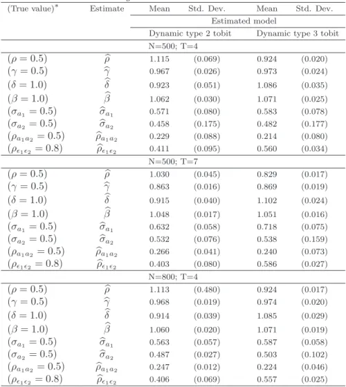
(13) and a dynamic linear regression. The parameter restrictions listed in Table 2 can be tested using a standard likelihood ratio or Wald test. We now present Monte Carlo simulations to study the small sample behavior of the maximum likelihood estimator of the type 2 and type 3 tobit models.. 5. Monte Carlo study. The data are generated according to the following “true” model d∗it = ρdi,t−1 + δwit + ηi + ²1it ,. (18). ∗ yit = γyi,t−1 + βxit + αi + ²2it ,. (19). where wit and xit are generated according to the standard normal distribution and are independent of each other, (²1it , ²2it ) is generated according to the bivariate normal distribution with mean zero and covariance matrix defined as in equation (8) (first matrix). The individual effects (ηi , αi ) are generated independently of (²1it , ²2it ) according to the bivariate normal distribution with mean (di0 , yi0 ) and covariance matrix defined as in equation (8) (second matrix). The dependent variables of the equation of interest and the selection rules are defined as in equations (3-5), i.e., both the type 2 and type 3 tobit are considered. The true parameter values are δ = β = 1, σa1 = σa2 = σ²2 = 0.5, σ²1 = 1, ρa1 a2 = 0.5, ρ²1 ²2 = 0.8, and two sets of values are chosen for ρ and γ, namely ρ = γ = 0 when the model is static, and ρ = γ = 0.5 when the model is dynamic. All dynamic and static data generating processes considered include individual effects. Given these values of the parameters, sample selection is not constant over time, i.e. the selection outcome dit (or sit ) has a rather high within standard deviation (around 0.40) for the (dynamic and static) type 2 and type 3 tobit. Furthermore, the censoring rate over the whole period, for both models, is approximately 40% and 50% in the dynamic and the static settings respectively. Finally, the correlation between the individual effects and the initial conditions for the type 2 and type 3 tobit is 0.70 and 0.80 in the selection equation, and 0.80 for both models in the equation of interest. To summarize, the data generating process (DGP) at the initial period is standard type 2 (type 3) tobit while the remaining period DGP is dynamic type 2 (type 3) tobit with endogenous initial conditions correlated with the individual effects, and accounting for selection bias correction (SBC). The static DGP is obtained by setting the true values of ρ, γ to 0. The estimation results of ρ, γ, δ, β, σa1 , σa2 , ρa1 a2 and ρ²1 ²2 based on 200 replications are shown. 11.

(14) in Tables 3-8 for the following sample sizes: N = 500 and T = 4, N = 500 and T = 7, and N = 800 and T = 4. We report the mean and standard deviation over the replications of these estimates.10 In each replication, the estimation is based on T − 1 periods, the first one being the initial period. We study the small sample behavior of the maximum likelihood estimator (MLE) of the abovementioned parameters when the model is both correctly and incorrectly specified. More specifically, when the DGP is dynamic, misspecification includes a dynamic model with no individual effects but SBC; with individual effects, exogenous initial conditions and SBC; with individual effects, endogenous initial conditions but no SBC; and a static model with individual effects and SBC. When the DGP is static, misspecification includes a static model with no individual effects but SBC; with individual effects but no SBC; and a dynamic model with no individual effects but SBC, and with individual effects and endogenous initial conditions correlated with the individual effects and SBC. We now discuss the Monte Carlo results.. 5.1. The MLE behavior when the model is correctly specified. The mean and standard deviation of the MLE of ρ, γ, δ, β, σa1 , σa2 , ρa1 a2 and ρ²1 ²2 , when the model is correctly specified, are reported in Table 3. The MLE of δ and β in both the dynamic and static type 2 and type 3 tobit is biased towards zero. The bias does not exceed 2% and 0.7% for δ and β in the type 2 tobit, and 3.5% and 0.8% in the type 3 tobit. There is no clear pattern of bias reduction as either T or N increases. In all cases but the dynamic type 2 tobit with N = 800 and T = 4, the estimate of β is on average closer to the true value than that of δ. In both the type 2 and type 3 tobit, the estimates of δ and β are closer to the true values in the static case than in the dynamic case, except in the dynamic type 2 tobit with N = 800 and T = 4 where the pattern shows up the other way round in the estimate of δ. From this, we can conclude that it is more difficult to estimate accurately the coefficients of the strictly exogenous explanatory variables in both the selection equation and the equation of interest of dynamic panel data sample selection models than those of their static counterparts. The MLE of ρ and γ is also biased towards zero in both the dynamic type 2 and type 3 tobit. The bias does not exceed 2% and 4.7% for ρ and γ in the type 2 tobit, and 3.5% and 4.2% in the type 3 tobit. Like δ and β, there is no clear pattern of bias reduction as either T or N increases, and the MLE bias of ρ and γ is overall larger than that of δ and β. As a result, we can state that it is more difficult to estimate accurately the coefficients of the lagged dependent variables than 10 We do not report the estimate results of σ ²1 (for the type 3 tobit), σ²2 , and the additional parameters of equations (6) and (7).. 12.

(15) those of the strictly exogenous variables in both the selection equation and the equation of interest of dynamic panel data sample selection models. In both models, σa1 and σa2 are much less accurately estimated than ρ, γ, δ and β, even though their bias remains towards zero. For both models, the bias is smaller in the static case than in the dynamic case. In all cases but, for σa1 when N = 500 and T = 7, the bias is smaller in the type 2 tobit than in the type 3 tobit. The two models exhibit different patterns in the bias reduction as T increases. Indeed, the type 2 tobit shows an increase in the MLE bias of σa1 and σa2 which is more pronounced for σa1 than it is for σa2 . The increase in the MLE bias of σa1 , as T increases, confirms the results by Rabe-Hesketh et al. (2005) that show that the MLE of the standard deviation of the individual effects in random-effects probit models is biased away from zero for large cluster size T , with a bias that ranges from 19% for T as small as 10 to 178% for T as large as 500. The type 3 tobit on the other hand shows a decrease in the bias of the MLE of σa1 and σa2 which is more pronounced for σa1 than it is for σa2 . As N increases, the bias reduction pattern is not clear cut, especially in the type 3 tobit. Finally, in both models, the MLE of ρa1 a2 is biased away from zero with a bias of about 25%, while that of ρ²1 ²2 is biased away from zero in the type 2 tobit and towards zero in the type 3 tobit. This bias decreases only slightly as T increases, while there is no clear pattern of reduction as N increases. To summarize, we can state that, when the model is correctly specified, the MLE bias of the parameters of panel data sample selection models is very small for a sample size as large as the one considered in the Monte Carlo study. The “two-step” Gauss-Hermite quadrature used to approximate the likelihood function works very well, even for a number of integration points, in each step, as small as 2. However, the standard deviations of the individual effects and the sample selection terms are less accurately estimated than the remaining parameters of Table 3. Accuracy in the estimates can be gained by either increasing the number of integration points or using adaptive Gauss-Hermite quadrature in the spirit of Rabe-Hesketh et al. (2005).11 We now discuss the behavior of the MLE when the model is incorrectly specified.. 5.2. The MLE behavior when the model is incorrectly specified. The mean and standard deviation of the MLE of ρ, γ, δ, β, σa1 , σa2 , ρa1 a2 and ρ²1 ²2 , when the model is incorrectly specified, are reported in Tables 4-8. More specifically, we study the finite 11 In the study by Rabe-Hesketh et al. (2005), adaptive Gauss-Hermite quadrature is shown to work better than normal Gauss-Hermite quadrature in static random-effects probit models when T or the equicorrelation is very large. The use of adaptive Gauss-Hermite quadrature can be generalized to sample selection models but is beyond the scope of this study.. 13.

(16) sample bias of the MLE when we fail to account for individual effects, when we assume exogenous initial conditions and when we fail to correct for selection bias. We also study the case where a static model is estimated under a dynamic DGP and vice versa. All DGPs considered include individual effects. 5.2.1. No individual effects. Table 4 reports the mean and standard deviation of the MLE of ρ, γ, δ, β and ρ²1 ²2 when the individual effects, while being present in the DGP, are ignored in the estimation of the model, i.e., σa1 , σa2 and ρa1 a2 are all assumed to be zero. The MLE of β remains biased towards zero in all cases. In other words, the MLE bias of the coefficient of the strictly exogenous explanatory variable in the equation of interest is unaffected if we fail to account for individual effects. This result holds regardless of the type of the selection rule, and regardless of whether the model is dynamic or static. The MLE of δ also remains biased towards zero in the type 3 tobit and in the static type 2 tobit with a larger bias than that of β. In the dynamic type 2 tobit, however, the MLE of δ is biased away from zero with a bias that is always larger than 15%. Hence, unlike β, when we fail to account for individual effects, the MLE behavior of the coefficient of the strictly exogenous explanatory variable in the selection equation differs according to the type of the selection rule and according to whether the model is dynamic or static. In the dynamic version of the model, the MLE of ρ and γ is biased away from zero and upwards in all cases, with a bias that gets as large as 61% in the type 2 tobit, and 55% in the type 3 tobit. This bias is reduced fairly substantially (by about 9%) as T increases but remains very high, and is unchanged as N increases. In other words, when estimating the dynamic version of the model and failing to account for individual effects, the coefficients of the lagged dependent explanatory variables, in both the selection equation and the equation of interest, are overestimated. In the dynamic panel data discrete choice model, this phenomenon is known as spurious state dependence (Heckman, 1981a), i.e. too much credit is attributed to past event as a determinant of current event if intertemporal correlation in the unobservables is not accounted for. Finally, the MLE of ρ²1 ²2 is biased away from zero with a bias of about 25% in the static case, and about 35% in the dynamic case. There is no clear pattern of bias reduction as either T or N increases.. 14.

(17) 5.2.2. Exogenous initial conditions. Table 5 reports the mean and standard deviation of the MLE of ρ, γ, δ, β, σa1 , σa2 , ρa1 a2 and ρ²1 ²2 when the initial conditions, while being endogenous and correlated with the individual effects in the DGP, are assumed to be exogenous, i.e., bs1 and br1 are assumed to be zero. In both the type 2 and type 3 tobit, the MLE bias of δ and β increases by about 6% with respect to the case of the DGP but remains fairly small, less than 9% in the type 2 tobit, and less than 11% in the type 3 tobit. As for the MLE of ρ and γ, their bias remains substantially large compared to the case where the individual effects are ignored. Accounting for individual effects but assuming exogenous initial conditions also results in a spurious state dependence situation.12 Hence, we can state that, in order for the coefficients of the lagged dependent explanatory variables to be accurately estimated, the correlation between the initial conditions and the individual effects must be taken into account: controlling for individual effects only is not sufficient. As T increases, the MLE bias of ρ and γ, in both the type 2 and type 3 tobit, decreases by about 10% but remains substantially large, while, as N increases, the bias remains the same. Finally, the MLE bias of ρa1 a2 and ρ²1 ²2 is higher than in the DGP case, and that of σa1 and σa2 is comparable to that of the same parameters in the DGP case. 5.2.3. No selection bias correction. The mean and standard deviation of the MLE of ρ, γ, δ, β, σa1 and σa2 are reported in Table 6 when we do not correct for the selection bias, i.e., we assume ρa1 a2 and ρ²1 ²2 to be zero. In both the type 2 and type 3 tobit and regardless of whether the model is dynamic or static, the MLE bias of the coefficients of the lagged dependent and strictly exogenous explanatory variables is unaffected. This result always holds for δ and β when the strictly exogenous explanatory variables in the selection equation and in the equation of interest are not at all or only slightly correlated. When they are highly correlated, Monte Carlo results not reported here show that the MLE of the coefficients in the equation of interest are biased downwards while that of the coefficients in the selection equation remains unaffected. The most notable change occurs in the MLE of σa1 which, in all cases, becomes biased away from zero, while that of σa2 remains, in all cases but in the dynamic type 2 tobit, biased towards zero. 12 Although the term spurious state dependence was used in the context of discrete choice models, we use it in our study to explain the overestimation of the coefficients of the lagged dependent explanatory variables in both the selection equation and the equation of interest.. 15.

(18) 5.2.4. Static model estimated under a dynamic DGP. The MLE of δ, β, σa1 , σa2 , ρa1 a2 and ρ²1 ²2 are reported in Table 7 when a static model is estimated under a dynamic DGP, i.e., ρ and γ are assumed to be zero. In both the type 2 and type 3 tobit, the MLE of δ is biased away from zero, with a bias that is no less than 30%, while the MLE of β remains biased towards zero but with a larger bias than in the DGP case. Furthermore, the standard deviations of the individual effects are overestimated and their MLE bias gets as large as 200% for σa1 , and 100% for σa2 . In other words, when past event is a determinant of current event and is left out of the explanatory variables, too much credit is attributed to the individual effects as a determinant of current event. This is the reverse phenomenon of the spurious state dependence. Finally, ρa1 a2 and ρ²1 ²2 are biased away from zero with a bias of approximately 25% and 45% respectively. 5.2.5. Dynamic model estimated under a static DGP. We estimate two types of dynamic models under a static DGP. The first one ignores the individual effects, and the second one accounts for individual effects that are correlated with endogenous initial conditions. In other words, the first type assumes σa1 , σa2 and ρa1 a2 to be all zero while the second one makes no restriction assumptions on the parameters of the model. The mean and standard deviation of the MLE of ρ, γ, δ, β, σa1 , σa2 , ρa1 a2 and ρ²1 ²2 are reported in Table 8. In both cases, the MLE of δ and β are biased towards zero in the type 2 and type 3 tobit. However, the bias for δ is larger when we do not account for the individual effects than when we account for them. The most notable difference between the two cases lies in the estimates of the coefficients of the lagged dependent explanatory variables. They are positive, around 0.10 for ρ and 0.15 for γ, and significantly different from zero when we do not account for the individual effects. In other words, ignoring the individual effects results in attributing credit to past event as a determinant of current event while the former does not condition at all the latter. This is an extreme case of the spurious state dependence mentioned earlier. When we account for individual effects that are correlated with endogenous initial conditions, these estimates become very close to zero, their true value, and the standard deviations of the individual effects are biased towards zero. Hence, when estimating a dynamic panel data model, regardless of whether the DGP is dynamic or static, the issues of properly accounting for the individual effects and treating the initial conditions must be taken care of. As for ρa1 a2 , it is biased away from zero in both the type 2 and type 3 tobit, while ρ²1 ²2 is biased away from zero in the type 2 tobit, and in the type 3 tobit with no individual effects. When individual effects that are correlated with endogenous initial conditions. 16.

(19) are accounted for, ρ²1 ²2 is biased towards zero in the type 3 tobit.. 6. Application. To illustrate our method we proceed to estimate a dynamic type 3 tobit model that explains the amount of product innovation. Innovation surveys distinguish two types of product innovations, those new to the firm (incremental) and those new to the market (radical). The importance of each type of product innovation is measured by the share in total sales of innovative sales. But from the way the questionnaire of the survey is formulated, we only observe the latter if we observe the former. Equation (1) determines whether enterprise i is an incremental product innovator at period t (d∗it > 0). In this case, the actual share of sales of incremental product innovations (eq. (5)) is positive, and the share of sales of radical product innovations (eq. (3)) and the full set of regressors included in the vector xit are observed. When enterprise i is not an incremental product innovator, the shares of sales of incremental (dit ) and radical (yit ) product innovations are equal to zero, and only the set of regressors included in the vector wit is observed. The dynamic type 3 tobit is implemented using the same data as in Raymond et al. (2006). They are collected by the Centraal Bureau voor de Statistiek (CBS) and stem from three waves of the Dutch Community Innovation Survey, CIS 2 (1994-1996), CIS 2.5 (1996-1998) and CIS 3 (19982000), merged with data from the Production Survey (PS). The population of interest consists of Dutch manufacturing enterprises with at least ten employees and positive sales at the end of the period covered by the innovation survey. We consider enterprises that existed in 1994, survived (at least) until 2000 and took part in the three innovation surveys, resulting in a balanced panel of 861 enterprises. Table 9 shows descriptive statistics and the description of the dependent and explanatory variables of the model. For instance, the average share in total sales of products new to the firm is rather small (29%), and that of products new to the market is even smaller (6.5%). These two variables are logit-transformed in order to make them lie within the set of real numbers.13 The specification of the model is as follows. The current share in total sales of products new to the firm is explained by the lagged share in total sales of products new to the firm, lagged size and relative size.14 Besides lagged size, the current share in total sales of products new to 13 The share of sales of products new to the firm takes on the values 1 for innovators that are newly established. They are replaced by 0.9999 in the logit transformation. Furthermore, the share of sales of products new to the market takes on the value 0 for some incremental product innovators. They are replaced by 0.0001 in the logit transformation. 14 In the innovation survey, firms are asked whether they have product and/or process innovations, or incomplete and abandoned innovation activities during the whole period under study, while size and sales are measured only at the end of the period. Hence, all the cross-sectional studies on the determinants of innovation have this unsatisfactory feature of explaining the probability of being an innovator (during the whole period) by size or relative size (at the. 17.

(20) the market is explained by the lagged share in total sales of products new to the market and dummy variables capturing demand pull, proximity to science, innovation cooperation, non-R&D performers, subsidies, and a continuous R&D intensity variable. Table 10 presents the estimation results of four versions of the type 3 tobit, namely a static model with unobserved individual effects, a dynamic model with no unobserved individual effects, a dynamic model with individual effects and endogenous initial conditions but ignoring the selection bias, and a dynamic model with individual effects and endogenous initial conditions correcting for selection bias.15 The hypotheses of the first three models are tested against those of the fourth one, and rejected using a likelihood ratio test at 1% level of significance. Hence, the preferred model is dynamic with individual effects and endogenous initial conditions correcting for selection bias. The results suggest that, in all four versions of the model, lagged size affects positively and significantly the current share of sales of incremental innovations. The current share of sales of radical innovations is positively and significantly affected by R&D intensity, performing R&D continuously, demand pull, innovation cooperation, subsidies while, ceteris paribus, non-R&D performers are less successful than R&D performers in terms of generating innovative sales from radical innovations. Sample selection operates through the individual effects and the idiosyncratic errors in the static case, and only through the idiosyncratic errors in the dynamic case. In the static case, too much of a role is attributed to the individual effects in that their standard deviations, as well as the correlation between them, are overestimated. Finally, the coefficients associated with the lagged dependent variables are positively and statistically significantly estimated in the three dynamic cases. However, they are overestimated when the individual effects are not accounted for or when the individual effects are accounted for but exogenous initial conditions are assumed. A dynamic type 2 tobit was also estimated using information only from a binary variable, indicating whether a firm is an incremental product innovator or not, for the selection equation and using the same equation of interest. As expected, the results (not reported in the paper) show that the parameters of the equation of interest are (slightly) less accurately estimated but similar to those of the type 3 tobit.. 7. Conclusion. We have proposed a simple method to implement the maximum likelihood estimator of dynamic panel data sample selection models. The method consists in writing the likelihood function condiend of the period). Taking lagged size or relative size as an explanatory variable in the panel data context overcomes this problem. 15 A dynamic model with unobserved individual effects and exogenous initial conditions was also estimated. The results, not reported in the paper, are similar to those of the dynamic model with no individual effects.. 18.

(21) tional on the individual effects which are then “integrated out” with respect to their joint normal distribution. We have handled the two-dimensional indefinite integral involved in the likelihood function using “two-step” Gauss-Hermite quadrature, and solved the initial conditions problem using the approach of Wooldridge (2005). The resulting likelihood function encompasses a wide range of likelihood functions of panel data models whose estimation can be achieved by simply making restriction assumptions on the parameters of the dynamic panel data sample selection model. These assumptions can be tested using a standard likelihood ratio or Wald test. In order to assess the quality of the Gauss-Hermite quadrature, and hence that of the maximum likelihood estimator, we have conducted a Monte Carlo study and obtained the following results. First, under the data generating process, the maximum likelihood estimator works very well, even for a number of integration points, in each step of the Gauss-Hermite quadrature, as small as 2. The estimator bias of the coefficients of the lagged dependent and strictly exogenous explanatory variables, as well as that of the standard deviations of the individual effects is very small for a sample size as large as the one considered in the Monte Carlo study. The sample selection terms, however, are less accurately estimated when the number of integration points is very small. Secondly, too much of a role is attributed to the lagged dependent variables as a determinant of the current dependent variables when either the individual effects or the correlation between the initial outcome and the individual effects are not taken into account. Thirdly, the selection bias really matters when the explanatory variables in the selection equation and in the equation of interest are highly correlated, otherwise it can be safely ignored. Fourthly, when the lagged dependent variables condition the current dependent variables and are left out of the explanatory variables, too much of a role is attributed to the individual effects as a determinant of the current dependent variables. Finally, when estimating a dynamic panel data model, regardless of whether the true model is dynamic or static, the individual effects and the correlation between the initial outcome and the individual effects must be taken into account, otherwise a situation of spurious state dependence will arise even under its extreme form. In this latter case, credit is attributed to the lagged dependent variables as a determinant of the current dependent variables while the former do not condition at all the latter. We have applied the method to estimate a dynamic type 3 tobit model of incremental and radical product innovations. The estimation results confirm those of the Monte Carlo study. More specifically, the effect of past incremental and radical product innovations on current incremental and radical product innovations is overestimated when either the individual effects or the correlation between the initial conditions and the individual effects are not accounted for. We also find that too much importance is attributed to the individual effects as a determinant of current in19.

(22) cremental and radical product innovations when past incremental and radical product innovations do not enter the set of explanatory variables. Finally, the estimation results of the model with no selection bias correction are similar to those of the model with a selection bias correction, even though the latter model is shown, using a likelihood ratio test, to be the preferred one. Our approach can be, in a straightforward manner, extended to estimate by maximum likelihood panel data sample selection models with more than two equations, that include a lagged dependent explanatory variable and individual effects in each equation. For instance, our approach can handle the estimation of dynamic panel data type 4 and type 5 tobit models with individual effects.. 20.

(23) Appendix A. “Two-step” Gauss-Hermite quadrature. Consider the dynamic panel data type 2 tobit model defined by equations (1-4) and (6-7), and consider expressions (10) and (11). Assume that the vectors (²1it , ²2it )0 and (a1i , a2i )0 are independent of each other, and independently and identically distributed over time and across individuals following a normal distribution with mean zero and covariance matrix given in equation (8). The likelihood function of individual i, starting from t = 1 and conditional on the regressors and the initial conditions, is obtained by “integrating out” the individual effects (equation (9)). The likelihood function of individual i conditional on the individual effects is written in equation (12) with σ²1 being normalized to 1 for identification reasons. The expression of the bivariate normal distribution of a1i and a2i is written as. g(a1i , a2i ) = (2πσa1 σa2 ). −1. −1 ¢ −1 ¡ 2 1 − ρ2a1 a2 2 e 2(1−ρa1 a2 ). „. a2 1i 2 σa 1. −2ρa1 a2. a1i a2i σa1 σa2. a2. «. + σ22i. a2. .. (20). Hence, equation (9) can be written as Z. ∞. 2. −a2 2i 2. e 2σa2 (1−ρa1 a2 ). Li = −∞. µ ¶¸dit T · Y 1 yit − Bit − a2i φ H(a2i )da2i , σ²2 σ²2 t=1. (21). where H(a2i ) is written as. H(a2i ) = (2πσa1 σa2 ) ×. T Y. −1. ¡ ¢ −1 1 − ρ2a1 a2 2. Z. ∞. e. −a2 1i 2 (1−ρ2 2σa a1 a2 ) 1. e. 1 (1−ρ2 a1 a2 ). “ ρa1 a2. a1i a2i σa σa 1 2. −∞. " Ã (1−dit ). Φ [− (Ait + a1i )]. t=1. Φ. ρ. Ait + a1i + σ²1²²2 (yit − Bit − a2i ) p 2 1 − ρ2²1 ²2. ”. !#dit da1i .. (22). Equation (21) can be approximated using “two-step” Gauss-Hermite quadrature which states that Z. ∞. 2. e−z f (z)dz '. −∞. M X. wm f (am ),. (23). m=1. where wm and am are respectively the weights and abscissas of the Gauss-Hermite quadrature, the tables of which are formulated in mathematical textbooks (e.g. Abramovitz and Stegun, 1964), and M is the total number of integration points. The larger M , the more accurate the GaussHermite quadrature. The “two-step” Gauss-Hermite quadrature consists, in the first step, in approximating equation (22) using equation (23). In the second step, a second approximation is applied to equation (21) where H(a2i ) is replaced by its first-step Gauss-Hermite approximation. The approach is described as follows.. 21.

(24) Consider the variable change z1i =. σa1. √. a1i 2(1−ρ2a. 1 a2. ). so that da1i = dz1i σa1. p. 2(1 − ρ2a1 a2 ). Equa-. tion (22) is then written as √. Z. 2 H(a2i ) = 2πσa2 ×. T Y. ∞. e. 2 −z1i. e. 1 1−ρ2 a1 a2. “ ” √ a ρa1 a2 z1i 2(1−ρ2a1 a2 ) σa2i 2. −∞. q h ³ í(1−dit ) Φ − Ait + z1i σa1 2(1 − ρ2a1 a2 ). t=1. " Ã. × Φ. Ait + z1i σa1. p. (24). ρ. 2(1 − ρ2a1 a2 ) + σ²1²²2 (yit − Bit − a2i ) 2 p 1 − ρ2²1 ²2. !#dit dz1i. and can be approximated using equation (23) by √. M 2 X H(a2i ) ' wm 2πσa2 m=1. ×. T Y. ( e. 1 1−ρ2 a1 a2. “ √ ρa1 a2 am 2(1−ρ2a. a. 1 a2. ) σa2i. ”. 2. q í(1−dit ) h ³ Φ − Ait + am σa1 2(1 − ρ2a1 a2 ). t=1. " Ã. × Φ. Ait + am σa1. p. (25). ρ. 2(1 − ρ2a1 a2 ) + σ²1²²2 (yit − Bit − a2i ) 2 p 1 − ρ2²1 ²2. !#dit   . ,. where wm and am are the weights and abscissas of the first-step Gauss-Hermite quadrature with M being the total number of integration points. Consider the second variable change z2i =. σa2. √. a2i 2(1−ρ2a1 a2 ). so that da2i = dz2i σa2. p 2(1 − ρ2a1 a2 ).. Replacing equation (25) into equation (21) yields Ã !#dit " p Z T 1 − ρ2a1 a2 ∞ −z2 Y 1 yit − Bit − z2i σa2 2(1 − ρ2a1 a2 ) Li ' φ e 2i π σ ²2 σ²2 −∞ t=1 ( M T q h ³ í(1−dit ) X Y × wm e2ρa1 a2 z2i am Φ − Ait + am σa1 2(1 − ρ2a1 a2 ) p. m=1. " Ã. × Φ. Ait + am σa1. p. t=1 ρ. 2(1 − ρ2a1 a2 ) + σ²1²²2 (yit − Bit − z2i σa2 p 2 1 − ρ2²1 ²2. p. 2(1 − ρ2a1 a2 )). (26) !#dit   . dz2i. which can be approximated using again equation (23) by  " Ã !#dit p P T Y 1 − ρ2a1 a2 X yit − Bit − ap σa2 2(1 − ρ2a1 a2 ) 1 Li ' φ wp  π σ²2 σ ²2 p=1 t=1 ( M T q h ³ í(1−dit ) X Y × wm e2ρa1 a2 ap am Φ − Ait + am σa1 2(1 − ρ2a1 a2 ) p. m=1. Ã. × Φ. Ait + am σa1. p. t=1 ρ. 2(1 − ρ2a1 a2 ) + σ²1²²2 (yit − Bit − ap σa2 p 2 1 − ρ2²1 ²2. 22. p. 2(1 − ρ2a1 a2 )). (27) !dit   . ,.

(25) where wp and ap are the weights and abscissas of the second-order Gauss-Hermite quadrature with P being the total number of integration points. Using equations (9), (13), (14) and (20), the random-effects individual likelihood function of the type 3 tobit can be derived similarly to yield equation (16).. 23.

(26) References Abramovitz M, Stegun I. 1964. Handbook of Mathematical Functions with Formulas, Graphs, and Mathematical Tables. National Bureau of Standards Applied Mathematics, US Government Printing Office: Washington, D.C. Ai C, Chen C. 1992. Estimation of a fixed effects bivariate censored regression model. Economics Letters 40: 403–406. Amemiya T. 1984. Tobit models: A survey. Journal of Econometrics 24: 3–62. Arellano M, Honoré B. 2001. Panel data models: Some recent developments. In Handbook of Econometrics, Heckman JJ, Leamer E (eds). North Holland: Amsterdam. Askildsen JE, Baltagi BH, Holm˚ as TH. 2003. Wage policy in the health care sector: A panel data analysis of nurses’ labour supply. Health Economics 12: 705–719. Butler JS, Moffitt R. 1982. A computationally efficient quadrature procedure for the one-factor multinomial probit model. Econometrica 50: 761–764. Chamberlain G. 1980. Analysis of covariance with qualitative data. Review of Economic Studies 47: 225–238. Dustmann Christian, Rochina-Barrachina Mar´ıa Engracia. 2000. Selection correction in panel data models: An application to labour supply and wages. IZA Discussion Paper No. 162. Gayle G-L, Viauroux C. 2007. Root-n consistent semiparametric estimators of a dynamic panelsample-selection model. Journal of Econometrics . Forthcoming. Greene W. 2004a. The behaviour of the maximum likelihood estimator of limited dependent variable models in the presence of fixed effects. Econometrics Journal 7: 98–119. Greene W. 2004b. Convenient estimators for the panel probit model: Further results. Empirical Economics 29: 21–47. Guilkey DK, Murphy JL. 1993. Estimation and testing in the random effects probit model. Journal of Econometrics 59: 301–317. Hausman JA, Wise DA. 1979. Attrition bias in experimental and panel data: The Gary income maintenance experiment. Econometrica 47: 455–474. Heckman JJ. 1979. Sample selection bias as a specification error. Econometrica 47: 153–162.. 24.

(27) Heckman JJ. 1981a. Heterogeneity and state dependence. In Studies in Labor Markets, Rosen S (ed). University of Chicago Press. Heckman JJ. 1981b. The incidental parameters problem and the problem of initial conditions in estimating a discrete time-discrete data stochastic process. In Structural Analysis of Discrete Data with Econometric Applications, Manski CF, McFadden D (eds). MIT Press: Cambridge, MA. Heckman JJ, MaCurdy TE. 1980. A life cycle model of female labour supply. Review of Economic Studies 47: 47–74. Honoré BE, Kyriazidou E. 2000. Estimation of tobit-type models with individual specific effects. Econometric Reviews 19: 341–366. Hsiao C. 2003. Analysis of Panel Data. 2nd edn. Cambridge University Press. Kyriazidou E. 1997. Estimation of a panel data sample selection model. Econometrica 65: 1335– 1364. Kyriazidou E. 2001. Estimation of dynamic panel data sample selection models. Review of Economic Studies 68: 543–572. Lancaster T. 2000. The incidental parameter problem since 1948. Journal of Econometrics 95: 391–413. Lee M-J. 2001. First-difference estimator for panel censored-selection models. Economics Letters 70: 43–49. Magnac T. 2004. Panel binary variables and sufficiency: Generalizing conditional logit. Econometrica 72: 1859–1876. Neyman J, Scott EL. 1948. Consistent estimates based on partially consistent observations. Econometrica 16: 1–32. Nijman T, Verbeek M. 1992. Nonresponse in panel data: The impact on estimates of a life cycle consumption function. Journal of Applied Econometrics 7: 243–257. Rabe-Hesketh S, Skrondal A, Pickles A. 2005. Maximum likelihood estimation of limited and discrete dependent variable models with nested random effects. Journal of Econometrics 128: 301–323.. 25.

(28) Raymond W. 2007. The dynamics of innovation and firm performance: An econometric panel data analysis. Ph.D. thesis, Maastricht University. forthcoming. Raymond W, Mohnen P, Palm F, Schim van der Loeff S. 2006. Persistence of innovation in Dutch manufacturing: Is it spurious? CESifo Working Paper No. 1681. Ridder G. 1990. Attrition in multi-wave panel data. In Panel Data and Labor Market Studies, Hartog J, Ridder G, Theeuwes J (eds). North-Holland, Amsterdam. Rochina-Barrachina ME. 1999. A new estimator for panel data sample selection models. Annales d’Economie et de Statistiques 55-56: 153–182. Semykina A, Wooldridge JM. 2005. Estimating panel data models in the presence of endogeneity and selection: Theory and application. unpublished working paper, Michigan State University. Vella F. 1998. Estimating models with sample selection bias: A survey. The Journal of Human Resources 33: 127–169. Vella F, Verbeek M. 1999. Two-step estimation of panel data models with censored endogenous variables and selection bias. Journal of Econometrics 90: 239–263. Verbeek M. 1990. On the estimation of a fixed effects model with selectivity bias. Economic Letters 34: 267–270. Wooldridge JM. 1995. Selection corrections for panel data models under conditional mean independence assumptions. Journal of Econometrics 68: 115–132. Wooldridge JM. 2005. Simple solutions to the initial conditions problem in dynamic nonlinear panel data models with unobserved heterogeneity. Journal of Applied Econometrics 20: 39–54. Zabel JE. 1992. Estimating fixed and random effects models with selectivity. Economics Letters 40: 269–272.. 26.

(29) 27. binary. binary. Semykina and Wooldridge (2005). Gayle and Viauroux (2007). dynamic. static. static. static. fixed. fixed. fixed. fixed. fixed-effects and pooled 2SLS with SBC SIV; SMD. kernel weighted LS and IV. semiparametric FD. labor supply participation decision n.a.. labor supply participation decision. n.a.. n.a.. n.a.. tion decision. n.a. labor supply equation labor supply participa-. n.a.. n.a. n.a.. n.a. n.a. nonresponse equation. labor supply equation n.a.. attrition equation. Selection equation. n.a.. wage equation. labor supply equation. n.a.. n.a.. n.a.. n.a. wage equation wage equation. n.a.. n.a. n.a.. n.a. n.a. consumption equation. wage equation n.a.. earnings equation. Application Equation of interest. based on the pairwise differenced equation of interest.. ics. † The individual effects of the selection and the outcome equation are random and fixed respectively. †† The selection equation is static. ‡ In these studies, the estimation is. ML, OLS, SBC, STLS, FGLS, LS, CML, MD, IV, GMM, FD, SIV, SMD and 2SLS respectively stand for maximum likelihood, ordinary least squares, selection bias correction, symmetrically trimmed least squares, feasible generalized least squares, least squares, conditional maximum likelihood, minimum distance, instrumental variable, generalized method of moments, first difference, sieve instrumental variable, sieve minimum distance and two-stage least squares. ∗∗ Only the selection (or attrition) equation allows for dynam-. ∗. binary. kernel weighted GMM. censored. fixed. Askildsen et al. (2003)‡. OLS with SBC OLS with SBC; CML MD with SBC; kernel weighted. kernel weighted LS. Lee (2001)‡. dynamic. fixed. fixed random fixed. fixed. binary. static. static dynamic∗∗ static. static. ML pooled OLS with SBC. Kyriazidou (2001)‡. Rochina-Barrachina (1999)‡ Vella and Verbeek (1999) Dustmann and Rochina-Barra-. random fixed. kernel weighted LS; STLS. binary binary; censored binary. Kyriazidou (1997)‡. static static. ML STLS ML; FGLS with SBC. hybrid† fixed random. IV; IV and GMM with SBC. binary. Zabel (1992) Wooldridge (1995). static static dynamic∗∗. ML ML ML; OLS with SBC. fixed random. random. Estimation method∗ of the equation of interest. binary; censored. binary binary; censored. Verbeek (1990) Ai and Chen (1992) Nijman and Verbeek (1992). static static dynamic∗∗. Individual effects. Honor´ e and Kyriazidou (2000)‡. binary censored binary. Heckman and MaCurdy (1980) Ridder (1990). Dynamic or static. Table 1: Studies on sample selection models with panel data. china (2000)‡. binary. censored binary. Hausman and Wise (1979). Selection rule. Study.

(30) Table 2: Panel data models encompassed in the dynamic type 2 and type 3 tobit models Restricted model. Parameter restrictions Initial conditions∗∗ Sample selection. Individual effects∗. The general model is dynamic type 2 (type 3) tobit† ††. Dynamic type 2 (type3) tobit Dynamic type 2 (type3) tobit. σa1 6= 0;σa2 6= 0;. bs1 = br1 = 0;. present. exogenous. selection bias correction. σa1 = σa2 = 0;. bs1 = br1 = 0;. ρ²1 ²2 6= 0; ρa1 a2 6= 0;. ρ²1 ²2 6= 0;ρa1 a2 6= 0;. absent. exogenous. selection bias correction. σa1 6= 0; σa2 6= 0;. bs1 6= 0; br1 6= 0;. ρ²1 ²2 = ρa1 a2 = 0;. present. endogenous. no selection bias correction. Dynamic probit (type 1 tobit) + dynamic linear regression. σa1 6= 0; σa2 6= 0;. bs1. present. exogenous. no selection bias correction. Dynamic probit (type 1 tobit) + dynamic linear regression. σa1 = σa2 = 0;. bs1 = br1 = 0;. ρ²1 ²2 = ρa1 a2 = 0;. absent. exogenous. no selection bias correction. σa1 6= 0; σa2 6= 0;. n.a.. ρ²1 ²2 6= 0; ρa1 a2 6= 0;. n.a.. ρ²1 ²2 6= 0; ρa1 a2 6= 0;. n.a.. ρ²1 ²2 = ρa1 a2 = 0;. Dynamic probit (type 1 tobit) + dynamic linear regression. Static†† type 2 (type 3) tobit. =. br1. = 0;. present Static type 2 (type 3) tobit. ρ²1 ²2 = ρa1 a2 = 0;. selection bias correction. σa1 = σa2 = 0; absent. selection bias correction. Static probit (type 1 tobit) + static linear regression. σa1 6= 0; σa2 6= 0;. Static probit (type 1 tobit) + static linear regression. σa1 = σa2 = 0;. present. no selection bias correction n.a.. absent. ρ²1 ²2 = ρa1 a2 = 0; no selection bias correction. ∗. 0r The individual effects, when present, may be correlated (b0s 2 6= 0; b2 = 0) with the explanatory variables. ∗∗ When the model is static (ρ =. 0r 6= 0) or uncorrelated (b0s 2 = b2 γ = 0) the initial conditions prob-. lem is not an issue, so bs1 = br1 = 0. † The general model contains individual effects and the initial conditions are endogenous and correlated with the individual effects. †† “Hybrid” models with a static selection and a dynamic equation of interest (and vice versa) can also be estimated using our approach.. 28.