SLA violation prediction : a machine learning perspective

(1)

Universit´e de Montr´eal

SLA Violation Prediction: A Machine Learning Perspective

par Reyhane Askari Hemmat

Département d’informatique et de recherche opérationnelle Faculté des arts et des sciences

Mémoire présenté à la Faculté des arts et des sciences en vue de l’obtention du grade de Maˆıtre ès sciences (M.Sc.)

en informatique

Octobre, 2016

c

(2)

Résumé

Le cloud computing réduit les coûts de maintenance des services et permet aux utilisateurs d’accéder à la demande aux services sans devoir être impliqués dans des détails techniques d’implémentation. Le lien entre un fournisseur de services cloud et un client est régi par une Validation du Niveau Service (VNS) qui définit pour chaque service le niveau et le coût associé. La VNS contient habituellement des paramètres spécifiques et un niveau minimum de qualité pour chaque élément du service qui est négocié entre les deux parties.

Cependant, une ou plusieurs des conditions convenues dans une VNS pourraient ˆ

etre violées en raison de plusieurs problèmes tels que des problèmes techniques occa-sionnels. Du point de vue d’apprentissage automatique, le problème de la prédiction de violation de la VNS équivaut à un problème de classification binaire.

Nous avons exploré deux modèles de classification en apprentissage automatique lors de cette thèse. Il s’agit des modèles de classification de Bayes na¨ıve et de Forêts Aléatoires afin de prédire des violations futures d’une certaine tâche utilisant ses traits caractéristiques. Comparativement aux travaux précédents sur la prédiction d’une violation de la VNS, nos modèles ont été entraˆınés sur des ensembles de données réels introduisant ainsi de nouveaux défis. Nous avons validé le tout en utilisant Google Cloud Cluster trace comme avec l’ensemble de données.

Les violations de la VNS étant des évènements rares (∼ 2.2%), leur classification automatique reste une tâche difficile. Un modèle de classification aura en effet une forte tendance à prédire la classe dominante au détriment des classes rares. Pour répondre à ce problème, il existe plusieurs méthodes de ré-échantillonages telles que Random Over-Sampling, Under-Sampling, SMOTH, NearMiss, One-sided Se-lection, Neighborhood Cleaning Rule. Il est donc possible de les combiner afin de ré-équilibrer le jeu de données.

Mots clés: Cloud Computing, Validation du Niveau Service, Apprentissage Automatique, Classification Déséquilibrée, Forêts Aléatoires, Classification de Bayes Na¨ıve

(3)

Summary

Cloud computing reduces the maintenance costs of services and allows users to access on demand services without being involved in technical implementation details. The relationship between a cloud provider and a customer is governed with a Service Level Agreement (SLA) that is established to define the level of the service and its associated costs. SLA usually contains specific parameters and a minimum level of quality for each element of the service that is negotiated between a cloud provider and a customer.

However, one or more than one of the agreed terms in an SLA might be violated due to several issues such as occasional technical problems. Violations do happen in real world. In terms of availability, Amazon Elastic Cloud faced an outage in 2011 when it crashed and many large customers such as Reddit and Quora were down for more than one day. As SLA violation prediction benefits both user and cloud provider, in recent years, cloud researchers have started investigating models that are capable of prediction future violations. From a Machine Learning point of view, the problem of SLA violation prediction amounts to a binary classification problem.

In this thesis, we explore two Machine Learning classification models: Naive Bayes and Random Forest to predict future violations using features of a submitted task. Unlike previous works on SLA violation prediction or avoidance, our models are trained on a real world dataset which introduces new challenges. We validate our models using Google Cloud Cluster trace as the dataset.

Since SLA violations are rare events in real world (∼ 2.2%), the classification task becomes more challenging because the classifier will always have the tendency to predict the dominant class. In order to overcome this issue, we use several re-sampling methods such as Random Over-Sampling, Under-Sampling, SMOTH, NearMiss, One-sided Selection, Neighborhood Cleaning Rule and an ensemble of them to re-balance the dataset.

Keywords: Cloud Computing, Service Level Agreements, Machine Learning, Unbalanced Classification, Random Forest, Naive Bayes

(4)

List of Figures

2.1 A depiction of a cloud system. . . 5

2.2 Cloud architecture and layered model: Hardware, Infrastructure, Platform and Application layers.. . . 6

2.3 Hybrid Cloud uses the infrastructure of two or more of the Public, Private or Community clouds. . . 9

2.4 Cloud Service Model: Three well-know cloud service model are IaaS, PaaS and SaaS providers. . . 14

2.5 SLA Life Cycle. . . 19

3.1 Dart chart: A graphical illustration of bias-variance trade-off. Con-sider a classification problem as throwing darts at a dart-board. If darts land in very different parts of the board, the model has “high variance”. If their mean is close to the center of the board, the model has “low bias”. Similarly, “low variance” and “high bias” can be de-fined. The above four dart boards corresponds to these situations (Moore and McCabe, 1989). . . 25

3.2 Left: the model is underfitted or equivalently has high bias. The reason is that we are trying to approximate a second order polyno-mial function using a linear function. Right: the model is overfitted because a high order polynomial function is used. Although the er-ror on the training set is close to zero, the model has a high variance. Middle: the model is just fitted. The Figure is adopted from Bishop (2006). . . 26

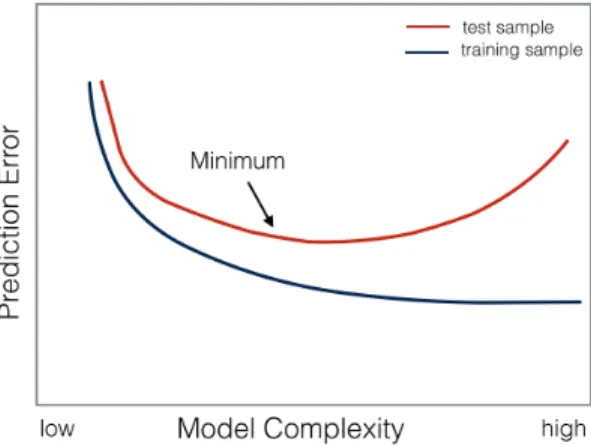
3.3 Test and training error as the function of model complexity. Figure is adopted from Murphy (2012). . . 28

3.4 Left: A confusion matrix; The table contains information about ac-tual and predicted targets of a binary classifier. Right: A graphical illustration of the confusion matrix; Red and Green are indicating the real classes while the dotted line corresponds to the threshold of a classifier. The right side of the dotted line is labeled as positive and the left side is labeled as negative. . . 29

(8)

3.5 In an ROC curve, the best ideal model would go straight up to left-upper corner and then straight to the right-upper corner. An untrained model with no discrimination is the diagonal one. Usually all classifiers are somewhere between the ideal one and the one with no power. . . 31

5.1 Google’s cluster trace dataset ERD (Entity Relationship Diagram). The dataset contains the above five different tables. This ERD is used to define and find violated tasks based on the definition in Section 5.1.1 . . . 37

5.2 The state transition diagram of a task on Google Cluster machines (Reiss et al., 2011). . . 38

5.3 The Figure shows 500 snapshots of the requested, available, assigned and used memory of the cluster. . . 40

5.4 In a single model, the complete dataset is given to the model in one iteration. In bagging, the dataset is divided into several sets randomly sampled with replacement from the original dataset. The sets are then fed to the model in parallel. In boosting, random sampling with replacement over weighted data is used. The data is sequentially given to a set of weak learners.. . . 42

5.5 Bayesian network representation of the naive Bayes classifier. Ac-cording the the graph representation, conditioned on the class Ck,

xi’s are independent of each other. . . 47

5.6 A graphical illustration of a Decision Tree: Classification starts from the top node towards leaves by testing the Outlook. After moving to one of the left or the right subtrees, a test on Humidity or Wind determines the class label (Mitchell et al., 1997). . . 49

5.7 In a random forest, k different decision trees are trained using k different subsets of the dataset. During test time, a sample input point is fed to all trees and predictions P1..k are generated. A voting

is then applied on all predictions to make a single final prediction. . 51

6.1 A hierarchical depiction of different sampling methods and the mod-els used for each. The number associated with each methods indi-cates the F1 score. Other methods∗: Since the data is highly

un-balanced, the other models mostly overfit and learn to always pre-dict the most dominant class. These models include Naive Bayes, Naive Bayes One-Sided Selection, Naive Bayes Neighborhood Clean-ing Rule, Naive Bayes Random over samplClean-ing, Naive Bayes SMOTE and its variants. . . 58

(9)

6.2 ROC curves of different sampling methods imposed on the random forest algorithm. ROC curves represent the performance of binary classifiers over different cut-off points of the algorithm. The area un-der the curve is consiun-dered as a single number presenting the trade-off between sensitivity (true positive rate) and specificity (true negative rate). . . 59

6.3 A 2D t-SNE visualization of different under sampling methods. (a): No Resampling, (b): Random Under-Sampling, (c): One-Sided Se-lection, (d): Neighborhood Cleaning Rule, (e): Near-Miss 1, (f ): Near-Miss 2, (g): Near-Miss 3. . . 60

6.4 A 2D t-SNE visualization of different over sampling methods. (a): No Resampling, (b): Random Over-Sampling, (c): SMOTE Bor-derline 1 and 2, (d): SMOTE. Note that the similarity between (b) and (a) is because Random Over-Sampling, duplicates the existing points randomly. . . 61

6.5 A 2D t-SNE visualization of different combined sampling methods. (a): No Resampling, (b): SMOTE Tomek Links, (b): SMOTE ENN 61

6.6 The average contribution of each feature based on the best trained random forest algorithm. The average is taken over all test examples. 62

(10)

List of Tables

2.1 Components of a Web Service Level Agreement (Buyya et al., 2010). 17

2.2 An example of infrastructure SLA (Buyya et al., 2010). . . 17

2.3 An example of application SLA (Buyya et al., 2010). . . 18

5.1 The description and type of features used as the input for the clas-sification model. . . 39

5.2 Two sample examples (datapoints) from the dataset for each class: violated and un-violated. . . 39

6.1 Full results of Naive Bayes (NB) and Random Forest (RF) classi-fication algorithms with Under-Sampling techniques. Results are achieved using 3-fold cross validation. . . 55

6.2 The results of Random Forest (RF) classification algorithm with Over-Sampling methods. Results are achieved using 3-fold cross val-idation. . . 55

6.3 The results of Naive Bayes (NB) and Random Forest RF) classi-fication algorithms with combination of Over-Sampling and under-Sampling techniques. Results are achieved using 3-fold cross valida-tion. . . 55

(11)

List of Abbreviations

AWS Amazon Web Services

BaaS Backend as a Service DaaS Data as a Service

ERD Entity Relationship Diagram IaaS Infrastructure as a Service MSE Mean Square Error

NCR Neighborhood Cleaning Rule

NIST National Institute of Standards and Technology NaaS Network as a Service

PGA Parallel Genetic Algorithm PaaS Platform as a Service QoS Quality of Service

ROC Receiver Operating Characteristics SECaaS Security as a Service

SLA Service-Level Agreement SLO Service Level Objectives

SMOTE Synthetic Minority Over-sampling Technique STaaS Storage as a Service

SaaS Software as a Service

T-SNE T-Distributed Stochastic Neighbor Embedding VM Virtual Machines

WS Web Server

(12)

Acknowledgments

For the ancestors who paved the path before me, upon whose shoulders I stand. This is dedicated to my parents Ataollah and Zahra and to my brothers Mohammad Ali and Mohammad Hossein.

I would like to express my deepest gratitude to my supervisor Prof. Abdel-hakim Hafid for his unwavering support, collegiality, and mentorship throughout this thesis.

I must also acknowledge great help and support from my friend Mohammad Pezeshki.

(13)

1

Introduction

1.1 Motivation and Statement of the Problem

Cloud computing provides a convenient way to access different IT resources such as servers, storage, databases and a wide range of application services over the Internet. The main appeal of cloud computing is that users do not get involved in details of service management, hardware maintenance, or software licenses.

In recent years, cloud computing is becoming the most cost-effective and reliable way of building and deploying different IT services. The superiority of cloud com-puting comes from the fact that it provides extensive comcom-puting and storage ser-vices on scalable and dynamic environment. According toWang et al.(2010), cloud computing has five unique characteristics among other computing paradigms; (1) User-centric interfaces: cloud computing is accessed using simple and user-friendly environments, (2) On-demand service provisioning: based on user requirements of a service, different amounts of resources can be allocated, (3) QoS guaranteed offer: cloud computing guarantees a minimum level of Quality of Service (QoS), based of a Service Level Agreement (SLA), (4) Autonomous System: system management including both hardware and software are all done autonomously without involv-ing users, and (5) Scalability and flexibility: cloud computinvolv-ing allows upscalinvolv-ing or downscaling IT resources easily.

Among the above-mentioned cloud characteristics, in this thesis we particularly, focus on the Quality of Service and Service Level agreements in cloud computing. “Quality of service represents the set of those quantitative and qualitative charac-teristics of a distributed multimedia system necessary to achieve the required func-tionality of an application” (Vogel et al., 1995). In order to guarantee a minimum level of QoS, a careful management of IT resources is essential. However, due to systems’ complexities, the task of managing resources in an efficient way is a chal-lenging problem. Management of resources and handling variable volumes of user

(14)

requirements are a part of SLA between users and cloud providers.

QoS management involves helping users to find the required characteristics of the demanded service and adaptation of IT resources in such a way to respect SLA and to optimize the system performance and efficiency. Generally speaking, the problem of resource adaptation including resource reallocation in a complex system with an enormous number of tasks is an NP-hard problem (Darmann et al., 2010). Consequently, it is inevitable that QoS agreed in SLA not be always respected. In the case that the effective QoS does not comply with the minimum QoS agreed in SLA, QoS manager issues an instance of SLA violation.

QoS manager allocates different amounts of resources (CPU, memory, or stor-age) and also determines the agreements in SLA based on four sources of informa-tion: (1) The requested IT resources for each user task, (2) The available resources of the computing system, (3) Information about the minimum QoS agreed in SLA, and (4) The historical information about the system’s load. QoS manager, usually using a heuristic method, decides how to prevent SLA violation. For example, in the application of video streaming such as YouTube, QoS manager may delay the video by a few seconds in order to buffer and prevent interruption in the middle of video. On the other hand, in some other applications such as video conference of Google Hangouts, in which significant delay is not acceptable, QoS manager may reduce the resolution of video or the sound quality to prevent any violation of the service. Therefore, it is desirable to be able to predict when an SLA violation may occur beforehand.

SLA violation prediction benefits both cloud providers and customers. From a cloud provider’s point of view, SLA violation results in paying penalties in terms of both money and reputation. By predicting violations ahead of time, providers can reallocate the requests and resources to prevent future violations. All the process of resource allocation is done behind the scene; thus, from a customer point of view, better resource allocation results in a trustworthy provider. Moreover, customers would like to receive the service on demand and without any interruptions. Thus, a system in which a cloud provider or a third party could provide the prediction of SLA violations for the customer can be very insightful.

It is worth mentioning that violations do happen in the real world. As an example, Amazon Elastic Cloud faced an outage in 2011 when it crashed and many

(15)

large customers such as Reddit and Quora were down for more than one day1_.

1.2 Contributions

In this thesis, we propose to use Machine Learning in order to predict SLA violations. Violation prediction can be seen as a classification problem in the terminology of Machine Learning. A classifier predicts whether a coming request will be violated or not. Each request is presented to the model using five different features: the priority of the task, the requested amount of disk space, the requested amount of CPU, the requested amount of memory, and also scheduling class which indicates latency-sensitivity of the task. We explore Random Forest and Naive Bayes classifiers. For the Naive Bayes we also explore two assumptions over the features vector: Bernoulli and Gaussian distributions.

Previous research mostly relies on heuristic methods for prediction of violations. Although Machine Learning has been used in different areas of QoS management, the experiments are done mostly in very restricted setting which is not necessarily scalable to real world data. However, this research takes a systematic machine learning approach applied on real-world data that provides an insightful set of ex-periments. We use 20k records of Google Cloud Cluster trace dataset containing ∼ 97.8% unviolated and ∼ 2.2% violated examples. Thus, the dataset is highly unbalanced and the classification task becomes more challenging because the clas-sifier will always have the tendency to predict the dominant class. This problem usually biases the classifier to always predict no violation which is not desirable. We address this issue by using multiple classifiers aggregated and averaged in order to achieve a single reliable result. Specifically, in terms of algorithm, we use ran-dom forest classification model and in terms of data, we use different re-sampling methods.

We show that our proposed model achieves a remarkable performance of 99.88% accuracy2 _{in prediction of violations. In addition, by analyzing the model and}

vi-sualization of different re-sampling methods, we provide insightful and actionable

1. Amazon Elastic Compute Cloud (Amazon EC2). Available athttps://aws.amazon.com/ ec2/

(16)

information on how to overcome the skewness of the dataset and train unbiased clas-sification models. It is also worth mentioning that we extract human-interpretable results from the model which suggests that requested memory is the most corre-lated feature with violation occurrence. Finding the importance of each feature can then help the provider to implement a management system that can improve the performance of its cloud services.

1.3 Organization of this Thesis

In Chapter 2, we introduce fundamentals of Cloud Computing, its architecture, cloud’s service model and deployment models. We will also give a brief definition of Service Level Agreement and Quality of Service. In Chapters 3, we give a description of the terminologies and basic concepts in machine learning. We define different machine learning models such as classification and regression. We also present how the performance of a model is measured in machine learning.

In Chapter 4, we present an overview of existing contributions on SLA violation prediction; in particular, we present the limitations of these contributions and how our proposed model aims to overcome them. Chapter 5 presents the proposed method that is used to predict SLA violation. Chapter 6 presents the details of the evaluation and the implementation of our proposal. Finally, Chapter 7 concludes the thesis and presents future work.

(17)

2

Cloud Computing

Cloud computing is a new paradigm for providing various hosting services over the internet. It has recently become so prevalent that it is hard to picture using many services and applications without cloud computing. There has been many driving forces that has led to the popularity and advancement of cloud computing. Computing power and storage have had rapid development and the hardware cost has been decreased. The emergence of exponentially growing data, the necessity of a new business model and technology led to the concept of cloud computing. See Figure 2.1 for a graphical illustration of a cloud system.

Figure 2.1 – A depiction of a cloud system.

Cloud computing reduces the maintenance costs of the service and also allows users to access on demand services without being involved in technical implemen-tation details. Business owners do not need to plan ahead for provisioning and enterprises can start small and increase the resources as they grow.

According to the National Institute of Standards and Technology (NIST) (Mell and Grance,2011), the definition of cloud computing is: Cloud computing is a model for enabling convenient, on-demand network access to a shared pool of configurable computing resources (e.g., networks, servers, storage, applications, and services)

(18)

that can be rapidly provisioned and released with minimal management effort or service provider interaction.

In this chapter, we present the architecture of cloud and its service and deploy-ment models. Then cloud computing’s characteristics are presented and related technologies such as grid computing, utility computing and autonomic computing are briefly discussed. Finally, we will introduce the concept of Quality of Service and Service Level Agreements in cloud.

2.1 Cloud Architecture and Layered Model

To better understand cloud computing, we need to first describe the architecture of cloud. Cloud architecture is usually defined in a layered model. Modular and layered structures such as OSI model and cloud layered architecture simplify the separation and definition of different parts of the system and reduce management overheard.

The architecture of cloud consists of four layers (Zhang et al.,2010): Hardware, Infrastructure, Platform and Application. We briefly discuss these layers in the following sections.

Figure 2.2 – Cloud architecture and layered model: Hardware, Infrastructure, Platform and Application layers.

(19)

2.1.1 Hardware Layer

This layer mostly includes the physical hardware that actually runs the cloud. It is usually a networked collection of data centers connected through switches and routers. Inside data centers are racks of servers, storage arrays, cooling infrastruc-ture, power converters and backup generators (Zhang et al.,2010). Fault tolerance in this layer is managed via redundancy of several inexpensive physical hardware.

2.1.2 Infrastructure Layer

This layer is the foundation of Cloud Computing. It provides the virtualization technology that makes cloud flexible and scalable. Virtual machines (VMs) are deployed on hardware with different operating systems. A virtual machine creates logic structures that seem to operate just like the physical machine. Virtual ma-chines are created and deleted at will which enables users to have dynamic resource allocation and maximum resource utilization.

2.1.3 Platform Layer

This layer includes operating systems and web platforms on top of the infras-tructure layer. It provides a container for application development or APIs for cloud application development without the need to manage the hardware, virtual machines or operating systems. The cloud platform acts as a container where web applications with storage and database can be created.

2.1.4 Application Layer

The application layer is the most visible layer to end-users. Applications are accessed by users though a web portal. Cloud applications do not require the user to handle software upgrades and patches. Applications at this level are fast at processing real time data and are highly scalable.

(20)

2.2 Cloud Deployment Models

According to the NIST (Mell and Grance, 2011) definition of cloud, there are four cloud deployment models known as public, private, community and hybrid clouds. These four deployment models specify who is the customer of the services that are provided by these clouds.

2.2.1 Public Cloud

The services provided in a public cloud are open to use for general public, mean-ing customers that are external to the provider’s organization. The services can be free or in a pay as you go manner. The service can be sold, managed and operated by end-users, businesses or organizations. Public cloud service providers usually own and operate the infrastructure at their data center and access is generally, provided via the Internet.

2.2.2 Private Cloud

Private clouds are owned or leased by one large or mid size organization. They can be hosted externally or internally. The services are not in a pay as you go manner because the hardware, storage, network and the whole infrastructure is dedicated to the organization.

Security is a key aspect in private clouds (Mell and Grance, 2011). The usage of dedicated hardware, storage and network can ensure higher levels of security.

2.2.3 Community Cloud

Community clouds have shared infrastructures for a specific community that share a common goal (security, compliance, jurisdiction, etc.). They can be man-aged internally or by a third party and are hosted either internally or externally. Compared to a private cloud the costs can be shared in a community cloud and the services are provided in a pay as you go manner. On the other hand, compared to public cloud, a higher level of security that is more compatible with organizations is provided.

(21)

2.2.4 Hybrid Cloud

In hybrid clouds, the infrastructure is composed of two or more other cloud models (private, public or community) that will be separated from each other but bounded with a standard technology. They provide multiple benefits of different deployment models. Organizations can use a hybrid of public and private clouds to store sensitive information in a private cloud connected to an application that is deployed in a public cloud.

Public Cloud

Community Cloud

Private Cloud

Hybrid Cloud

Figure 2.3 – Hybrid Cloud uses the infrastructure of two or more of the Public, Private or Community clouds.

2.3 Cloud Computing Characteristics

According to NIST definition of cloud computing, a cloud system has five essen-tial characteristics; on demand self-service, broad network access, resource pooling, rapid elasticity and measured service (Mell and Grance,2011). There are also sev-eral common characteristics in cloud systems; service oriented, multi-tenancy and geographic distribution, to name a few. We briefly discuss each of these character-istics.

2.3.1 On Demand Self-service

On demand self service or automation is a property that enables customers to perform all actions needed to acquire or release a service without any human interaction and in a pay as you go manner. The transition usually takes place

(22)

immediately, although depending on the architecture and the resource availability of the provider it may be delayed (Zhang et al., 2010).

A customer does not need to have huge investment in a service from the start and can scale the required service up to a significant level without any disruption on host operations. Moreover, the traditional provisioning model for resources was based on the peak demand of the service whereas in a cloud system, resources are acquired on-demand which can considerably lower the costs. The customer is charged only for the resources used under a subscription-based billing method.

2.3.2 Broad Network Access

A cloud system should be accessible over a network. This characteristic is called Broad Network Access. Computing capabilities in a cloud system are available from a wide range of locations over the network and accessed through standard mechanisms.

Comparing to the mainframe era when resources were scarce and costly, nowa-days, broad network access of cloud systems has become possible (Williams,2012). The reason is that the network bandwidth and access has increased and also the cost associated with networks has decreased.

2.3.3 Resource Pooling

In a cloud system, providers offer a pool of computing, network, storage and services to various costumers. Providers have the flexibility of dynamically assign-ing the pooled resources and services to multiple customers. The customers will share resources adjacent to other customers (Zhang et al., 2010). This character-istic allows providers to manage their resources by maximizing resource utilization and minimizing the operating costs, power consumption and cooling. This leads to offering resources with considerable lower prices.

2.3.4 Rapid Elasticity

An elastic system can adapt to workload changes by provisioning and depro-visioning the resources in an autonomic way. Rapid elasticity is the ability of

(23)

fast provision and deprovision of resources such that available resources match the current requested resources as much as possible.

In a cloud system, provision of resources can be so quick that the resources can appear unlimited to the customer and provision can be performed in any quantity at any time.

2.3.5 Measured Service

In a cloud system, resource usage is automatically monitored, controlled and reported by using metering capabilities with some level of abstraction. The mea-surement tools provide both the provider and the customer an account of what has been used. This allows transparency between the provider and the customer.

2.3.6 Service Oriented

Cloud systems operate with a service-driven model. In such systems, service management and preferably autonomous service management are key aspects. Each provider offers the resources under an agreement called Service Level Agreement (SLA) (Casalicchio and Silvestri,2013). SLA can be negotiated between a provider and a customer and is an essential part of cloud systems to ensure maximum availability of services for customers. With a violation of SLA, the provider has to pay penalties, thus SLA assurance is a critical objective for every provider.

2.3.7 Multi-tenancy

Multi-tenancy is a property that allows a system to serve a single instance of a resource or application for multiple customers which are called tenants in this case (Krebs et al.,2012). This system requires secure physical and logical separation of resources which are controlled by one tenant in a shared environment. It is worth mentioning, that per-tenant reporting and quota management are key aspects in a multi-tenant system (Krebs et al., 2012).

The layered structure of cloud allows adding new features to the system by changing the entire infrastructure once for all customers whereas in a dedicated hardware per customer environment, changes need to be done per device (AlJahdali et al., 2014).

(24)

2.3.8 Geographic Distribution

As mentioned previously, one of the main characteristics of cloud systems is broad network access. Hence, to achieve higher performance, localization can be used. Many of cloud providers have data centers distributed around the world in order to gain the maximum service utility (Attiya and Welch,2004).

2.4 Related Technologies

Several technologies share close characteristics with cloud computing. We will briefly describe Grid Computing, Utility Computing and Autonomic Computing and discuss their common characteristics with Cloud Computing.

2.4.1 Grid Computing

According to Foster et al. (2008), grid computing is a resource provisioning model where computing resources are distributed. Usually large number of servers (nodes) are connected to each other through a network to form a grid. Large and computing-intensive workloads are sent to grid which are then shared between nodes in a paralleled manner. Thus, it requires software that can divide the compu-tation task into pieces. This rises the concern of software management or handling failure of a node.

Scalability and multi-tenancy are the shared features between cloud and grid computing. However, in cloud computing the resources are allocated and de-allocated on demand and at a more granular level by using virtualization (Foster et al.,2008). Virtualization amounts to running multiple operating systems and ap-plication on a single physical server. Cloud and grid computing both offer SLAs to provide resources for a guaranteed uptime. Storage computing in a grid is designed for data-intensive tasks. It is not financially preferred for storing small objects, but cloud computing can be implemented in non-grid environments (Foster et al.,

(25)

2.4.2 Utility Computing

According to Rappa (2004), Utility Computing is “the on-demand delivery of infrastructure, applications, and business processes in a security-rich, shared, scal-able, and standards based computer environment over the Internet for a fee”.

Utility computing is mostly used in cases where the peak of usage is rare. By using virtualization, it tries to minimize the operating costs while maximizing the actual usage of resources. Thus, the main leverage of utility computing is the economics (Degabriele and Pym, 2007).

Utility computing can be considered as the backbone of cloud computing but cloud computing provides more features and flexibility (Kaur and Singh, 2015). Cloud computing can be used internally in an organization. It also has unlimited scalability, utility based pricing, network access and on-demand self service.

2.4.3 Autonomic Computing

Autonomic computing is the self-managing feature of distributed computing. In autonomic computing, the control of the system, application and resources are done without human interaction thus removing the burden of management. The system adapts to unpredictable changes and hides the system’s complexity from the users (Kephart and Chess, 2003).

Autonomic computing reduces maintenance costs by hiding the system com-plexity. The autonomic feature is also included in cloud computing but with a different purpose. Autonomic resource allocation and SLA monitoring are two fea-tures of cloud computing but they aim to reduce the cost and maximize the resource utilization rather than reducing the complexity (Zhang et al., 2010).

2.5 Service Model

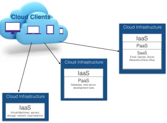
The service model architecture of cloud computing suggests that the resources provisioned in cloud be provided as services in an on-demand fashion. These ser-vices are usually grouped into three categories; Infrastructure as a Service (IaaS), Platform as a Service (PaaS), Software as a Service (SaaS). Each layer can be used as a service provider for the upper layer (Mell and Grance, 2011).

(26)

There are also other less popular service models for cloud such as; Network as a Service (NaaS), Storage as a Service (STaas), Security as a Service (SECaaS), Data as a Service (DaaS), Backend as a Service (BaaS) and etc. or the generally as called in Banerjee et al. (2011), Everything as a Service that are provided by cloud providers at different layers.

Cloud Infrastructure

IaaS Virtual Machines, servers, storage, network, load balancer

IaaS

PaaS

Database, web server, development tools

IaaS

PaaS SaaS

Email, Games, Social Networks,Online office

Cloud Clients

Figure 2.4 – Cloud Service Model: Three well-know cloud service model are IaaS, PaaS and SaaS providers.

2.5.1 Infrastructure as a Service (IaaS)

In the IaaS model, the infrastructure provider leases disk, CPU, memory, hard-ware, network and other infrastructure components to an end-user or other cloud providers. An IaaS provider handles tasks including backup, maintenance and re-siliency planning. Also, the administrative tasks are automated. The user has the ability to dynamically scale using virtualization technology but has no control over operating systems and applications that are running on the server (Mell and Grance,2011). Famous IaaS providers are Amazon Web Services (AWS), Windows Azure, Google Compute Engine and Rackspace Open Cloud.

2.5.2 Platform as a Service (PaaS)

(27)

infras-tools that are usually used for application development (Mell and Grance, 2011). Thus, the platform is used by end-users or software providers for deployment of software applications without the cost and complexity of acquiring and managing the underlying hardware and software layers. A user in PaaS can upgrade operating system features but has no control over the underlying cloud infrastructure such as operating systems, disk, CPU, memory, hardware and network. Famous PaaS providers are Appear IQ, Mendix, Amazon Web Services (AWS) Elastic Beanstalk, Google App Engine and Heroku.

2.5.3 Software as a Service (SaaS)

In the SaaS model, the software provider uses a platform or an infrastructure provider or uses its own infrastructure to deliver a software to end-users. SaaS removes the burden of maintenance, installation, acquisition, provisioning and li-censing of software (Mell and Grance, 2011). Organizations or individuals do not need to install the software on their data centers or on their computers. Instead, the software is available through a web browser or an API. The user has no control over the underlying infrastructure that is running the software such as operating systems, disk, CPU, memory, hardware, network. Most of the time, end-users do not even need to configure the software. Famous SaaS providers are Salesforce, Oracle, SAP, Intuit and Microsoft.

2.6 Quality of Service in Cloud Computing

“Quality of service represents the set of those quantitative and qualitative char-acteristics of a distributed multimedia system necessary to achieve the required functionality of an application” (Vogel et al., 1995). By measuring the QoS of a system, the performance can be improved and guaranteed in advance. Therefore, QoS measurement increases the reliability and availability of the system. In cloud systems, QoS is an essential aspect as cloud customers would like to have a measure of the cloud’s performance and a cloud provider would like to find the best trade off between the provided service and the cost. In the infrastructure level of cloud

(28)

computing, there are several QoS parameters that can be measured (Meegan et al.,

2012):

— Compute: availability, outage length, server reboot time.

— Network: availability, packet loss, bandwidth, latency, mean/max jitter. — Storage: availability, input/output per second, max restore time,

process-ing time, latency with internal compute resource.

Cloud providers guarantee the QoS with Service Level Agreements (SLAs). Also, Service Level Objectives (SLOs) are given as quantitative or qualitative parameters of an SLA such as throughput, availability and response time (Sturm et al., 2000). We discuss the definition of SLA and SLA management and life cycle in the following sections.

2.6.1 Service Level Agreements

The relationship between a cloud provider and a customer is governed with a Service Level Agreement (SLA). SLA is negotiated between parties and a level of the service, QoS and its associated costs are agreed upon. SLA usually contains specific parameters and a minimum level of quality for each element of the service that is negotiated between the provider and the customer (Casalicchio and Silvestri,2013). A common framework for SLA definition is web service-level agreement (WSLA) (Ludwig et al., 2003). Components of a WSLA is shown in Table 2.1.

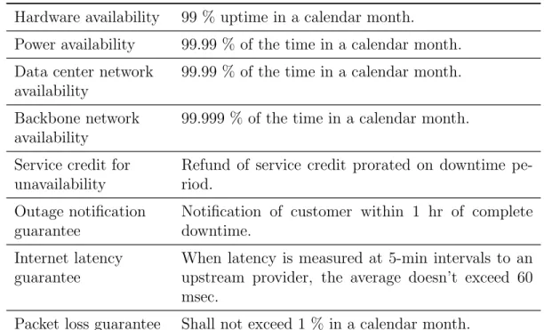
From an application hosting point of view, SLA has two different types: In-frastructure SLA and Application SLA. InIn-frastructure SLA guarantees a level of reliability on infrastructures such as power, data center, latency and etc. by ded-icating resources solely to the customer. An example is shown in Table 2.2. Ap-plication SLA is appropriate for hosting models on which multiple apAp-plications are co-located. In such a setting, cloud resources are available to applications accord-ing the application demands. Hence, in application SLA, cloud providers ensure meeting application demands. An example of application SLA is shown in Table

2.3.

For example, SLA can indicate a 99.99 % availability for requests of CPU, disk and memory. An SLA might also contain constraints on the response time for each request.

(29)

Table 2.1 – Components of a Web Service Level Agreement (Buyya et al.,2010).

Service-Level Parameter

Describes an observable property of a service whose value is measurable.

Metrics These are definitions of values of service properties that are measured from a service-providing system or com-puted from other metrics and constants. Metrics are the key instrument to describe exactly what SLA parame-ters mean by specifying how to measure or compute the parameter values.

Function A function specifies how to compute a metric’s value from the values of other metrics and constants. Func-tions are central to describing exactly how SLA param-eters are computed from resource metrics.

Measurement directives

These specify how to measure a metric.

Table 2.2 – An example of infrastructure SLA (Buyya et al., 2010).

Hardware availability 99 % uptime in a calendar month.

Power availability 99.99 % of the time in a calendar month. Data center network

availability

99.99 % of the time in a calendar month. Backbone network

availability

99.999 % of the time in a calendar month.

Service credit for unavailability

Refund of service credit prorated on downtime pe-riod.

Outage notification guarantee

Notification of customer within 1 hr of complete downtime.

Internet latency guarantee

When latency is measured at 5-min intervals to an upstream provider, the average doesn’t exceed 60 msec.

Packet loss guarantee Shall not exceed 1 % in a calendar month.

allocate the least amount of resources for each customer to reduce the cost of its server infrastructure. At the same time, the provider needs to avoid having

(30)

Table 2.3 – An example of application SLA (Buyya et al.,2010).

Service-level parameter metric

• Website response time (e.g., max of 3.5 sec per user re-quest).

Function • Latency of web server (WS) (e.g., max of 0.2 sec per request).

• Latency of DB (e.g., max of 0.5 sec per query)

• Average latency of WS = (latency of web server 1 + latency of web server 2 ) /2

• Website response time = Average latency of web server + latency of database

Measurement directive

• DB latency available via http://mgmtserver/em/latency.

WS latency available via

http://mgmtserver/ws/instanceno/latency Service-level

objective

• Service assurance.

Penalty • Website latency < 1 sec when concurrent connection < 1000.

• 1000 USD for every minute while the SLO was breached.

penalties due to failure of providing the agreed service. The failure of providing a service is called an SLA violation. The customer would like to receive the service on demand and without any interruptions. Despite these high availability rates, violations do happen in real world and have caused both the provider and the customer heavy costs (Leavitt, 2009).

2.6.2 SLA Management Life Cycle

According toGallizo et al.(2009) SLA management has a life cycle of six phases: — SLA Contract Definition

— Basic Schema with the Quality of Service (QoS) Parameters — SLA Negotiation

— SLA Monitoring

— SLA Violation Detection — SLA Enforcement

(31)

We will briefly describe these phases in the following subsections. Figure 2.5 illus-trates this life cycle.

1. Contract Definition 2. Basic Schema 3. SLA Negotiation 4. SLA Monitoring 5. SLA Violation Detection 6. SLA Enforcement

SLA Life Cycle

Figure 2.5 – SLA Life Cycle.

SLA Contract Definition

In this phase, the service and its corresponding price, QoS parameters with a basic schema and also the penalty policy is defined. SLAs are usually defined using standard or base templates or by customization of these base templates.

Basic Schema with the Quality of Service (QoS) Parameters

QoS parameters must be included in an SLA, covering different types of (virtu-alized) physical resources (e.g. for the network resources QoS parameters may be bandwidth, jitter, delay; for the computing resources the parameters may be CPU, memory, etc).

(32)

SLA Negotiation

In this phase a customer discovers a service provider that meets the customer’s needs. The terms and conditions of the SLA are negotiated and agreed upon in this phase. A cloud provider needs to analyze the SLA in terms of scalability, availability and performance of its services in order to avoid penalties before agreeing on the specification of SLA. By the end of this phase, parties start to commit to the agreement.

SLA Monitoring

In this phase, the provider’s performance in delivery of the service is measured against the contract. An essential part of SLA monitoring is to be able to predict violations enabling providers to reallocate the resources accordingly before occur-rence of violations.

SLA Violation Detection

In this phase the parameters inside SLA are calculated and any deviation is determined. In case of SLA violation, SLA enforcement is conducted.

SLA Enforcement

This phase is to enforce penalties for SLA violation. In this phase appropriate actions are taken place when the violation has been detected in the previous phase. The concerning parties are notified and penalty charges are taken place. After SLA enforcement, SLA might also terminate due to timeout or violation.

(33)

3

Prediction Models

Machine learning is the study and development of programs and algorithms that can learn from historical data and make prediction when exposed to new data. There are three general types of algorithms that are used to solve differ-ent problems in machine learning: supervised learning algorithms, unsupervised learning algorithms and reinforcement learning (Murphy, 2012).

— Supervised Learning aims to find a function that maps the input to the output given a labeled dataset1_.

— Unsupervised Learning aims to find the structures and patterns inside the input given an unlabeled dataset.

— Reinforcement Learning aims to find a function that outputs a sequence of actions that optimizes costs or rewards.

The focus of this thesis is on supervised learning. Consequently, after a re-view of some terminologies in machine learning, Supervised Learning is introduced in more details. Next, key concepts in machine learning such as Generalization, Bias-Variance Trade Off, Overfitting, Regularization, and Cross Validation are presented. Finally, we discuss how a model is evaluated in machine learning and specifically discuss Confusion Matrix, Accuracy, Precision and Recall, Fβ and ROC

curves.

3.1 Terminology

In this section, we introduce the basic terminology of machine learning which is used in the rest of this chapter. In a typical machine learning supervised task, a dataset is given in a set of rows and columns. Each row of the dataset corresponds to a single datapoint which is called a training example or a training instance.

1. In machine learning terminology the output variables or the targets are sometimes referred as labels. Thus, a dataset with inputs and their desired outputs is called a labeled dataset.

(34)

The columns are called input variables, features or attributes. Each datapoint is associated with one or more than one label(s), targets, or output variables.

The dataset is typically splitted into two sets; training set and test set. The training set is used to learn the underlying factors of variation in data, while the test set is used for the final evaluation. First, the model is trained given the training set and during testing, an example represented by its features is provided to the model and the output is the predicted label.

3.2 Supervised Machine Learning: Concepts

and Definitions

In supervised machine learning, two pieces of information are provided to the algorithm: a set of input instances X = {x1, x2, ..., xm} and a corresponding set of

targets Y = {y1, y2, ..., ym}. Typically, each of these m input instances contains a

set of n features x = {x1, x2, ..., xn}. Generally speaking, each feature xi can take

any value, either numerical (values are real numbers) or categorical (values are members of an unordered set). However, depending on the task at hand, features may be required to be converted to certain types.

There is always a true function f∗(.) that maps any possible x into the best possible y. However, we never have access to this unknown function. Accordingly, supervised learning amounts to approximating the function f∗(.) based on the information provided in the X and Y sets. The process of approximating f∗(.) using a function fθ(.) in which θ is a set of parameters is called learning.

Learning algorithms learn the parameters θ of the function fθ(.) by minimizing

the errors that the model makes. Formally, a function that maps the discrepancy between the output prediction of the model and the true target into a real number is called the loss function (Murphy, 2012).

If the true target y is a discrete variable, the prediction task is called Classi-fication. On the other hand, if y is continuous, the task is called Regression. In the following subsections, after formally introducing learning, we discuss these two types of supervised learning algorithms in more details.

(35)

3.2.1 Learning

Approximating function f∗(.) using function fθ(.) corresponds to extracting

the underlying factors of variation from data instances and mapping them to the output. These underlying factors could be a table of probabilities, a structure of a graph, or weights depending on which learning algorithm is used for knowledge discovery. Generally, learning amounts to finding the best parameters θ in order to minimize a loss function over all the examples in the dataset (Murphy, 2012). Therefore, the learning process can be formulated as follows,

ˆ θ = argminθ{ m X i=1 l(yi, oi; θ)}, (3.1)

in which ˆθ is the learned set of parameters, yi and oi are the target and output of

the model for the ith _sample.

3.2.2 Classification

In a supervised classification task, the prediction output y is from one of the total C distinct classes {1, 2, ..., C}. In order to get prediction for new examples, the model can simply output a class label or the output can be a set of probabilities. Each probability corresponds to one of C classes that indicates how probable it is that the unseen input x belongs to a specific class. In models that output probabilities, to get a discrete prediction out of the model, either the class with the highest probability is chosen or the class label is drawn by sampling from the output distribution.

3.2.3 Regression

Similar to a classification task, in regression problems, the goal is to learn a mapping function from an n-dimensional vector x into a real-valued number o as the prediction. Mean Square Error (MSE) is a common loss function used to measure the performance of regression models. Consequently, learning amounts to reducing the MSE between the model prediction and the true target which is

(36)

defined as follows, MSE(O, Y ) = n X i=1 ||oi− yi||2F (3.2)

The parameters of the model are then selected such that MSE is minimized.

3.3 Generalization

The goal of machine learning is to train models that are able to predict the labels for new unseen examples. As a result, generalization to new examples is an important side of each learning algorithm. We usually look for models that perform well on testing data as well as on training data. As a result, we need to prevent learning algorithms from simply memorizing training data; instead, these algorithms need to learn the underlying factors of variation.

3.3.1 Bias-Variance Trade off

In order to determine how accurate a model is, we need to understand what are the reasons behind errors. Bias and variance of a prediction model help us formally measure these errors. To define bias and variance over a model, we need to assume that we are able to train the same model multiple times with different randomly selected data points. In this thesis, each trained model is called a model instance. Errors in predictions that are caused by bias and variance are called error due to bias and error due to variance respectively (Sammut and Webb, 2011) (Geurts,

2002).

Bias corresponds to the distance between the expected prediction of the model and the true target (Wasserman,2013). Considering f (x) as the model, the bias is defined as follows:

bias = |E[f (x)] − y|2, (3.3)

(37)

model (Wasserman, 2013):

variance = |f (x) − E[f (x)]|2. (3.4) The total error of a model in terms of bias and variance is defined as follows:

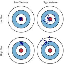
error = E[(f (x) − y)2] = bias2+ variance. (3.5) Given the limited amount of data, there is always a trade-off between bias and variance. The trade-off happens in a way that reducing one may lead to increasing the other. As a result, minimizing the total error requires a careful balance between bias and variance. A graphical illustration of this trade-off is shown in Figure 3.1.

Figure 3.1 – Dart chart: A graphical illustration of bias-variance trade-off. Consider a classi-fication problem as throwing darts at a dart-board. If darts land in very different parts of the board, the model has “high variance”. If their mean is close to the center of the board, the model has “low bias”. Similarly, “low variance” and “high bias” can be defined. The above four dart boards corresponds to these situations (Moore and McCabe, 1989).

3.3.2 Overfitting Problem

Overfitting is the case when a prediction model performs very good on the training data but achieves a significantly lower performance on the test data. This usually means that the model has memorized the whole training data including the noises instead of the underlying factors of variation that are essential for gener-alization. Overfitting could have different reasons including having small amount

(38)

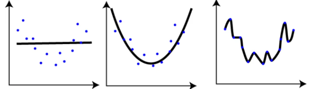
of data or too many model parameters (Bishop, 2006). Another reason for the problem of overfitting is unbalanced data which is one of the important aspects of this thesis. A typical example of overfitting is shown in Figure 3.2.

Figure 3.2 – Left: the model is underfitted or equivalently has high bias. The reason is that we are trying to approximate a second order polynomial function using a linear function. Right: the model is overfitted because a high order polynomial function is used. Although the error on the training set is close to zero, the model has a high variance. Middle: the model is just fitted. The Figure is adopted fromBishop(2006).

One potential reason for overfitting could be high capacity of a model. Model capacity is the ability of a model to fit a range of functions. Higher the model’s capacity is, the wider range of functions can possibly be approximated (Bishop,

2006). It is worth mentioning that dealing with overfitting or underfitting in such situations corresponds to the trade-off between bias and variance. As the model complexity increases, bias decreases while variance might increase in an overfitting setting.

Overfitting due to Unbalanced Data

If data contains a significantly large number of examples for one class and a few examples for the other(s), the data is called unbalanced or skewed. In such scenar-ios, classifiers may end up performing well on the majority class while performing poorly on other minorities. This type of overfitting simply happens because the classification objective assumes that errors from different classes have the same costs (Ganganwar, 2012). Consequently, fewer number of examples for one class leads to less error for that specific class.

(39)

3.3.3 Regularization

A group of different techniques used to avoid the problem of overfitting is called regularization. In most regularization techniques, some kind of prior knowledge is imposed on the model. For example, if number of examples in one class is not enough, resampling might be used to correct the class distributions. Or in some other cases, the model complexity might be controlled (Bishop,2006).

Usually, as parameters of a model grow in size, the model complexity increases which may lead to overfitting (Bishop, 2006). One of the basic solutions is to add a penalty term to the loss function in order to penalize models with high capacity. By adding this constraint, overfitting can be prevented as a result of preferring simpler models by the learning algorithm. Specifically, for supervised problems, the unregularized loss function in Equation 3.3 is altered with the following regularized one, ˆ θ = argminθ{ n X i=1 l(yi, oi; θ) + λJ (θ)}, (3.6)

where J (θ) is a constraint on the parameters and the coefficient λ controls the balance between two learning objectives.

3.3.4 Cross Validation

In order to find the parameters of the model that generalize the best, we need to know if the model has been overfit. Cross validation helps us to find an overfit model. Overfitting happens when the error rate in the training set decreases but the error on the test set increases. As shown in Figure 3.3, as we increase the complexity of the model, the error rate in the training set decreases but at some point the error in the test set passes the minimum and increases. When the error in the test set increases with higher model complexity the model is overfit.

In cross validation, the dataset is divided into training and validation sets. To increase the validity of the model, k-fold cross validation is used where the dataset is partitioned into k equal subsets. We define d as the complexity order of the model. For each order-d hypothesis class:

— Repeat k times:

(40)

Figure 3.3 – Test and training error as the function of model complexity. Figure is adopted fromMurphy(2012).

— Use the rest of the data points to find θ (model parameters). — Compute prediction error on the held-out subset.

— Average the prediction error over the k rounds/folds. Use this as the esti-mated true prediction error for order-d hypothesis class

The goal is to find d with the lowest estimated true prediction error. It is worth mentioning that k-fold cross validation increases the computation k-times. Thus, with larger datasets or complex models, smaller values of k is preferred.

3.4 Performance Evaluation

In this section, we introduce the common error metrics used for a classification: (1) Confusion Matrix, (2) Accuracy, (3) Precision and Recall, (4) Fβ Score, and (5)

ROC Curves (Stehman, 1997). Error metrics help us indicate how good the model will perform when exposed to unseen data. Thus, after the model is trained on the training set and the best performing2 _{model is chosen, it will be tested on an intact}

test set. This approach helps us select a model which will have good performance on unseen data.

(41)

3.4.1 Confusion Matrix

A confusion matrix is a table used to describe the performance of a classification model. To be able to construct the confusion table, the true targets must be available. As shown in Figure 3.4, a Confusion Matrix contains four values to describe the performance of a classification model: false positive, false negative, true positive, and true negative. False positive (resp. negative) is the number of mistakenly classified examples that are classified as 1 (resp. 0) where the actual targets are 0 (resp. 1). Similarly, true positive (resp. negative) is the number of correctly classified examples that are classified as 1 (resp. 0). Generally speaking, the first term (false or true) indicates if the classification result matches with the actual target. The second term (negative or positive) indicates the prediction of the classifier. Based on the confusion matrix, accuracy, precision and recall, Fβ

and ROC curves are defined.

Figure 3.4 – Left: A confusion matrix; The table contains information about actual and pre-dicted targets of a binary classifier. Right: A graphical illustration of the confusion matrix; Red and Green are indicating the real classes while the dotted line corresponds to the threshold of a classifier. The right side of the dotted line is labeled as positive and the left side is labeled as negative.

3.4.2 Accuracy

Accuracy indicates the number of correct predictions from all predictions made by a classification model. Formally, it is defined as,

accuracy = True positives + True negatives

(42)

3.4.3 Precision and Recall

Classification accuracy alone is not necessarily the best measurement to eval-uate the performance of a classifier and specifically in classification tasks with an imbalanced targets distribution. Suppose a case where we have a majority class (for instance 90 % of the targets belong to this class). A naive model that always pre-dicts the majority class achieves high accuracy (Ganganwar,2012). However, such a classification model that always outputs the same prediction is useless. Thus, accuracy could mislead us to prefer a model with high accuracy while there are cases where we can not merely rely on accuracy.

Precision and recall are two other useful measures that can help us evaluate a classification model more correctly. These two metrics are defined as follows,

precision = True positives

# of all positive predictions, (3.8) recall = True positives

# of all positive examples. (3.9)

3.4.4 F

β

Score

Precision and recall can also be seen as a measure of model exactness and model completeness respectively. However, in order to compare different models with different precisions and recalls, we need a balance between these two. The metric Fβ combines precision and recall into a single value such that different models are

compared more easily:

Fβ = (1 + β2) .

precision . recall

(β2 _{. precision) + recall}, (3.10)

where β is single number controlling the balance between precision and recall (Salton and Buckley, 1988).

3.4.5 Receiver Operating Characteristics (ROC) curves

(43)

perfor-nation threshold is the cut-off applied on the predicted probability of a test example that assigns it to a particular class. In an ROC curve, true positive and false posi-tive rates are plotted on vertical and horizontal axis respecposi-tively.

Figure 3.5 – In an ROC curve, the best ideal model would go straight up to left-upper corner and then straight to the right-upper corner. An untrained model with no discrimination is the diagonal one. Usually all classifiers are somewhere between the ideal one and the one with no power.

(44)

4

Related Works

The assurance of quality in cloud and proposed approaches approaches have been proposed since cloud computing. Researchers quickly realized that to achieve higher revenue, cloud providers can offer much more resources to customers than their available resources. This is due to the fact that not all customers use their maximum requested resources at the same time. Indeed, there is an underlying distribution that describes customers’ behaviors and can be used to manage the requests and resources. As described in section 2.6.2, SLA management provides a framework to effectively manage resource allocation to meet the requested QoS. Cloud is mainly considered to have three service models; Infrastructure as a Service (IaaS), Platform as a Service (PaaS) and Software as a Service (SaaS); in this thesis we mainly focus on the IaaS.

Different aspects of SLA management in IaaS can be categorized as follows: Load Prediction, Resource Scheduling, and SLA Violation Prediction. In this chap-ter we briefly describe the related works in each of these categories.

4.1 Load Prediction

A variety of contributions have been proposed for load prediction. Using re-gression based models, Barnes et al. (2008) proposed an extension of a regression based model for work load prediction in parallel applications. Zhang et al. (2011) proposed a model that predicts the characterization of tasks such as wait time and machine resource utilization on Google’s production clusters. Ganapathi et al.

(2010) proposed an extension of statistical models to predict resource requirements based on workloads in cloud computing. Carrington et al.(2003) introduced a new model to predict load values using a set of basis operations used in a specific appli-cation. Akioka and Muraoka (2004) and Dabrowski and Hunt (2008) used Hidden

(45)

Markov Models for host load predictions on large-scale computational grids. In a closely related work to this thesis, Di et al.(2014) proposed a recent work on host load predictions in a cloud environment using Google Compute Cluster dataset. Authors proposed a Bayesian model to predict the mean load over long-term and consecutive future time intervals. The key idea in this paper is to generate posterior distribution from the prior distribution and the recent fluctuations of load.

Ali-Eldin et al. (2012) proposed a provisioning model that monitors and also pre-dicts future loads. Based on the predicted loads, an autonomous elasticity module controls the number of allocated virtual machines and heuristically decreases it by a factor of three.

4.2 Resource Scheduling

In resource scheduling, the fundamental goal is to optimize the usage of infras-tructure while maintaining the highest QoS for provided services. In Zheng et al.

(2011), the authors use a parallel genetic algorithm (PGA) for the virtual machines scheduling task and load balancing in an IaaS cloud. Their method improves the availability and reliability of the cloud system.

In Zhang and Cao(2013), a resource management scheduling is modeled with a dynamic sequential decision model where future demands are foretasted. Resource management is done through basic operations such as switching on/off hosts, rent-ing remote cloud machines, makrent-ing machines standby and activatrent-ing machines. Grey Forecast Model is the core of their intelligent system where based on the historical data, the required number of Virtual Machines is predicted. It is worth mentioning that this work used synthetic data which is generated using a Poisson distribution in a simulation environment.

Wang and Vassileva (2007) manage different services based on SLA and feed-back from users in a peer-to-peer web application. In Wu et al. (2014), authors proposed a detection scheme that prevents unfair ratings to compete with other services. Alhamad et al.(2010) proposed an SLA-based trust model for cloud that selects the provider based on a selection scheme; in this scheme, although no vi-olation is predicted, the customers are grouped according to business needs and

SLA violation prediction : a machine learning perspective

Résumé

Summary

Contents

List of Figures

List of Tables

List of Abbreviations

Acknowledgments

1

Introduction

1.1

Motivation and Statement of the Problem

1.2

Contributions

1.3

Organization of this Thesis

2

Cloud Computing

2.1

Cloud Architecture and Layered Model

2.1.1

Hardware Layer

2.1.2

Infrastructure Layer

2.1.3

Platform Layer

2.1.4

Application Layer

2.2

Cloud Deployment Models

2.2.1

Public Cloud

2.2.2

Private Cloud

2.2.3

Community Cloud

2.2.4

Hybrid Cloud

2.3

Cloud Computing Characteristics

2.3.1

On Demand Self-service

2.3.2

Broad Network Access

2.3.3

Resource Pooling

2.3.4

Rapid Elasticity

2.3.5

Measured Service

2.3.6

Service Oriented

2.3.7

Multi-tenancy

2.3.8

Geographic Distribution

2.4

Related Technologies

2.4.1

Grid Computing

2.4.2

Utility Computing

2.4.3

Autonomic Computing

2.5

Service Model

2.5.1

Infrastructure as a Service (IaaS)

2.5.2

Platform as a Service (PaaS)

2.5.3

Software as a Service (SaaS)

2.6

Quality of Service in Cloud Computing

2.6.1

Service Level Agreements

2.6.2

SLA Management Life Cycle

3

Prediction Models