Economic and environmental comparison of a centralized and a decentralized heating production for a district heating network implementation

(1)

10th International Conference on System Simulation in Buildings, Liege, December 10-12, 2018

Economic and environmental comparison of a centralized and a

decentralized heating production for a district heating network

implementation

Thibaut Résimont

1

*, Queralt Altes-Buch

1

, Kevin Sartor

1

, Pierre Dewallef

1

(1) _{Energy Systems Research Unit, Aerospace & Mechanical Engineering Department, University of Liège,} Liège, Belgium

1. ABSTRACT

District heating networks seem to be a promising solution for heating delivery by using a centralized production unit instead of local gas boilers or heat pumps in each house. The use of several available heat sources, like waste incinerators for example, enables to reduce global primary energy consumption and to have a better control on pollutants emissions and greenhouse gases emissions than with a local heating production. The main drawback of district heating networks is the consequent initial investment cost for pipes and substations. It is thus interesting to achieve a fair comparison between a centralized heating production unit including a district heating network and a decentralized one with heating units in each house. The comparison is based on the IEA EBC Annex 60 case study made up of a small neighborhood of 24 dwellings combined with a greenhouse characterized by specific energy consumption profiles. For the centralized heating production, a waste incinerator and a gas boiler are considered as heating sources while gas boilers or heat pumps are taken into account for a decentralized heating production. In both cases, an economic and environmental study is achieved to determine the optimal scenario between a centralized and a decentralized heating production.

Keywords: District Heating Network (DHN), Dynamic modelling, Economic and environmental analysis

2. INTRODUCTION

In the frame of a worldwide environmentally-friendly policy looking for energy efficient solutions in order to reduce pollutants emissions and primary energy consumption, district heating technology exhibits some advantages compared to a decentralized heating production technology for the heating and cooling sector. 4th generation district heating systems enable the use of various combined heat and power (CHP) technologies from centralized heat pumps to residual heat from industrial processes or waste incinerators for example. Combined with thermal storages at strategic points along the network, this district system could be a promising solution for efficient energy models at an urban scale including renewable energies (UNEP, 2015). However, despite its existence since the 14th century (Rezaie et al., 2012), district heating is not widely developed in central Europe even though there is a large potential to harness. Indeed, in Eastern Europe for instance, district heating projects are more developed and have proven the technical feasibility and economic viability of this technology. Within the European Union, there are more than 5000 district heating systems in operation today with more than 40% in countries like Denmark, Sweden, Finland, Poland, Estonia, Latvia and Lithuania. On the other hand, there is a very small part of the heating demand which is covered by district heating in countries in Western Europe and especially in Belgium (Frederiksen et al., 2013). With an European policy for the short-term and mid-term scope based on smart, efficient and sustainable heating and cooling systems (EUROPA, 2016), there

(2)

is an increasing interest for projects in district heating with some new ones including the use of waste heat from incinerators or industrial processes. A local example in Liège (Belgium) is the waste incineration plant of Intradel which manages waste produced by more than 900,000 habitants and burns 370,000 tons per year of municipal waste. This energy could be valorized at a city scale such that a district heating network project (EcoSystèmePass project) is currently in progress for the 2020 horizon.

The main issue for the development of district networks is the large initial investment cost for required pipes and substations. Investments in district heating projects are generally limited by budget constraints and by a fear of underestimating the total costs for the project. The implementation of a simulation tool able to fulfill accurately some criteria as the assessment of the heating losses and pressure losses would be a solution to a current lack on the district heating network market. Currently, district heating networks are generally sized based on rules of good practice by quasi steady-state simulations. To take into account dynamic phenomena which have an impact on thermal and hydraulic losses, dynamic models would be useful as a basis for a decision tool. In the literature, many conventional dynamic models where pipes are modelled by finite volume elements can be found. However, these models are limited to small-scale networks because of their lack of numerical robustness for large district heating networks. Sartor et al. (2015) illustrated numerical problems related to conventional finite volume approaches developed by Gabrielaitiene et al. (2001) and many others. The development and validation of more adequate pipes components for a large scale application would therefore be useful to quantify as accurately as possible the physical behavior of a district heating network. These components with a stronger numerical robustness leading to an affordable computation time would answer to the current lack of simple dynamic models on the district heating network market. Based on these components, a simple simulation tool could be developed to assess economic and environmental criteria related to district heating networks.

3. THE SYSTEM MODEL

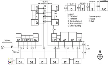
The case study used in this paper, depicted in Fig. 1, to assess the economic profitability to combine a waste incinerator to a district heating network is based on a test case developed by the IEA Annex 60 (IEA, 2018). An additional heat demand of a 1,000 m2 greenhouse is located at a distance of 100m of the heat source at the beginning of the network.

Figure 1: Sketch of the case study used in this paper based on the IEA Annex 60 Neighbourhood Case Study (IEA, 2018).

(3)

This case study is based on the EcoSystemePass project (cf. Acknowledgements) which aims to connect a greenhouse and a neighborhood of a few dwellings to a waste incinerator. Based on this configuration, it is required to model physically the components for each part of the network.

3.1. District Heating Network (DHN) model

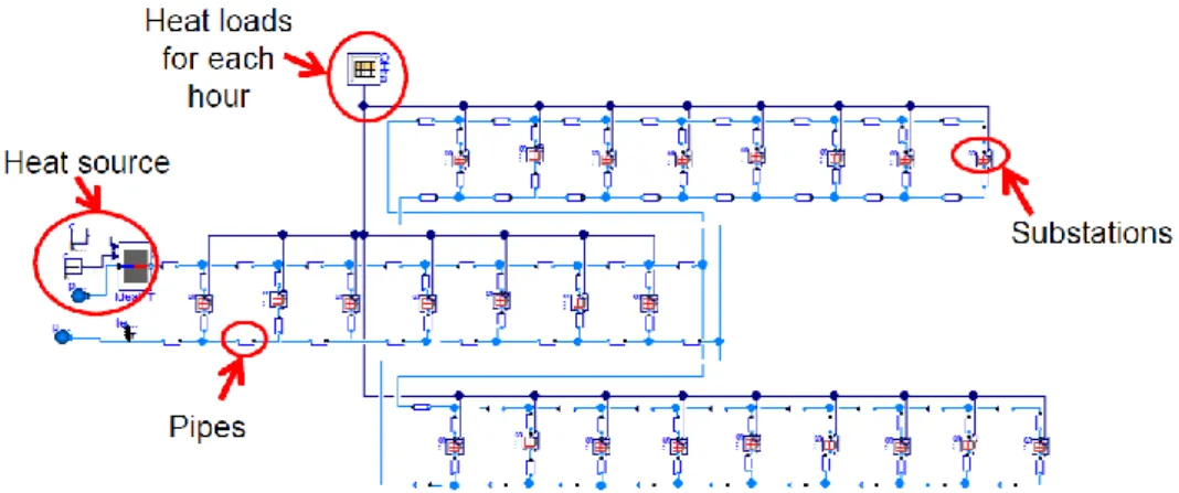
The modelling of the whole system requires the modelling of each component of the district heating network including the heat source, the pipes, the substations and the dwellings. This modelling can become quickly complex because of the large amount of partial differential equations in the mathematical model (even for a small network). Dynamic effects have to be taken into account in the dwellings but also in pipes where there are thermal inertia phenomena and a heat wave propagation time. For sake of simplicity, the detailed models of the dwellings and the greenhouse are not presented in this paper. The interested reader can refer to Résimont et al. (2018) and Altes-Buch et al. (2018) for an overview of the physical modelling used to determine hourly heating demands of the dwellings and the greenhouse. For the network modelling, these heating load profiles are used as inputs and a fixed temperature difference at the primary side of the substations is prescribed to determine the required mass flow rates in each substation. Assuming an ideal heat source able to provide any required mass flow rate without limitations for a prescribed temperature set point, the main remaining components to model are the pipes. The graphical model of the network developed in the dynamic simulation software Dymola is proposed in Fig. 2.

Figure 2: Thermo-hydraulic model of the district heating network developed in the dynamic simulation software Dymola

3.1.1. Pipes model

Pipes are used as connectors between the heating source and the substations and can reach a length of several hundreds or thousands of meters in large district networks. The main result is a heat wave propagation time from the heating source to the farthest points in the network of a few minutes (assuming a mean water velocity around 1 m/s in the pipes). Dynamic phenomena have thus a significant influence on the water temperature level in the pipes. Usual finite volume numerical methods dividing the pipes in discrete cells are commonly used for the thermo-hydraulic modelling of flows in pipes. However, these methods require large computational times proportional to the level of discretization of the pipes. A balance between a fair computation time and an accurate solution has thus to be found even though this compromise involves some limitations (Sartor et al., 2015). In the literature, an alternative pipe model, proposed by Van Der Heijde et al. (2017), is used to find an efficient solution both in terms of computation time and accuracy. This model is based on a plug flow

(4)

method where a delay time function is used to compute the residence time Δt of the fluid in the pipes. Overlooking about axial diffusion along the pipes and assuming a constant heat capacity of the pipes [J/K] as well as a constant thermal resistance [K/W] between the pipes and its surroundings, an analytical expression of the temperature at the outlet of the pipe can be directly deduced by Eq. (1). This equation is deduced from a combination of the energy and continuity equation. For a detailed physical explanation of the model and its mathematical development, the reader can refer to Van Der Heijde et al. (2017).

( )

₍₁₎

Equation (1) shows that the temperature at the outlet of the pipes is only dependent on the inlet temperature [°C], the surroundings temperature [°C] and the thermal properties of the pipes and . This simple method has already been validated on other test cases

and provides fair computation times for large scale district networks. Indeed, for this case study, dynamic simulations over a reference year get a computation time around only 3 hours compared to simulations of several days with finite volume methods. These relatively low computation times are also an advantage for operation planning on a day-to-day basis in order to predict the heating load profile as a function of daily weather conditions and to have a better instantaneous control monitoring over the entire network.

3.2. Heating source modelling

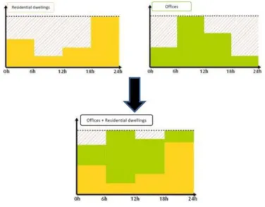
Centralized heating units usually run at full-load regime on a daily basis because they feed district heating networks with a global heating demand quite uniform over the day. Due to the different types of heating profiles related to various kinds of dwellings, the global heating consumption is fairly distributed over the day. This effect is represented in Fig.3.

Figure 3: Combination of the heating demand profiles of two types of dwellings (offices and residential dwellings)

As can be observed in Fig.3, the combination of both heating load profiles with offices, which have a significant heating consumption mainly during working hours, and residential dwellings whose the consumption is shifted during morning and evening periods, enables to have a global heating load profile more or less uniform over the day. This is the main advantage of centralized production enabling to run at full-load conditions most of the time such that a constant boiler efficiency can be considered all over the year.

(5)

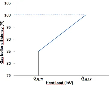
About decentralized heating units for local production, a variable load regime has to be taken into account, both for gas boilers and heat pumps, such that a variable efficiency/COP regime is used in this model. For the gas boiler, a variable efficiency included between 85 and 100% for respectively minimum and maximum heating loads is assumed. This efficiency varies linearly with the heating load, as represented in Fig. 4.

Figure 4: Variation of the gas boiler efficiency with the heating load

The gas boiler efficiency can be expressed mathematically as a linear function of the minimum and maximum efficiencies and the heating demand ̇:

( ̇)

̇ ̇ ̇ ( ) The average thermal efficiency ̅ of the gas boiler is defined by integrating the required

heating power ̇ divided by the primary energy consumption ̇ all over the year

on an hourly basis: ̅ ∫ ̇ ∫ ̇ ∫ ̇ ∫ ̇ ( ̇ ) ( )

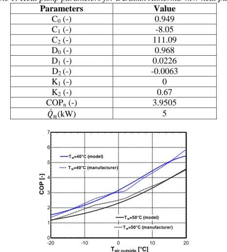
Concerning the COP of a heat pump, in addition to the influence of the part-load regime, it also varies with the temperature of the heat source as shown in Figure 5 (Ransy et al., 2017). The modelling of the heat pump is based on three polynomial laws developed by Bolther et al. (1999) in order to determine the COP and the full heating load capacity as a function of the heating source temperature, the required outlet temperature of the water and the part-load ratio for an air to water heat pump. Parameters for the polynomial laws are identified from manufacturers’ data such that each heat pump has specific parameters values and are based on nominal conditions. These nominal conditions are prescribed for the sizing of the machine. Nominal temperatures of 7°C and 35°C are respectively set up for the evaporator and the condenser of the heat pump. In this case study, a water set point temperature of 50°C and an air temperature based on weather data on an hourly basis are taken into account.

In this case study, reference heat pumps chosen for the performance assessment are Daikin

Altherma 4kW heat pumps whose polynomial coefficients have been identified and are

(6)

Table 1: Heat pump parameters for a Daikin Altherma 4kW heat pump

Parameters Value C0 (-) 0.949 C1 (-) -8.05 C2 (-) 111.09 D0 (-) 0.968 D1 (-) 0.0226 D2 (-) -0.0063 K1 (-) 0 K2 (-) 0.67 COPn (-) 3.9505 ̇ (kW) 5

Figure 5: Variation of the COP of the heat pump with the outdoor temperature (Ransy et al., 2017)

The 3 polynomial laws mentioned above are represented by the following set of equations. (4) with ₍ ₎ (5) ̇ ̇ ( ) ( ) (6) ̇ ̇ ( ) ( ) (7) with ̇ ̇ (8)

The first one is used to determine the COP at full load of the heat pump for a prescribed air temperature and a water set point temperature. The second one is an illustration of the maximum available heating capacity of the heat pump compared to the nominal heating load capacity. A computation of the heat pump performance at part-load operation is achievable using the third polynomial law represented by Eq. (7). For details about this polynomial model, the reader can refer to Bolther et al. (1999). Based on these 3 equations, an assessment of a mean COP over the year is computed by Equation (9) where ̇ is the electrical consumption of the compressor of the heat pump.

-20 -10 0 10 20 0 1 2 3 4 5 6 7 Tair,outside [°C] C O P [ -] Tw=50°C (model) Tw=50°C (model) Tw=50°C (manufacturer) Tw=50°C (manufacturer) Tw=40°C (model) Tw=40°C (model) Tw=40°C (manufacturer) Tw=40°C (manufacturer)

(7)

10th International Conference on System Simulation in Buildings, Liege, December 10-12, 2018 ̅̅̅̅̅̅ ∫ ̇ ∫ ̇ ∫ ̇ ∫ _{( ̇} ̇ ) ( )

About the centralized waste incineration, the bottleneck of this technology concerns pollutants emissions which have to be taken into account for prospective additional deNOx units. A set

of chemical equations modelling pollutants emissions from waste combustion is thus proposed in the next section to assess the prospective need to install a treatment unit for pollutants emissions.

3.2.1. Model for pollutants emissions assessment from waste incineration

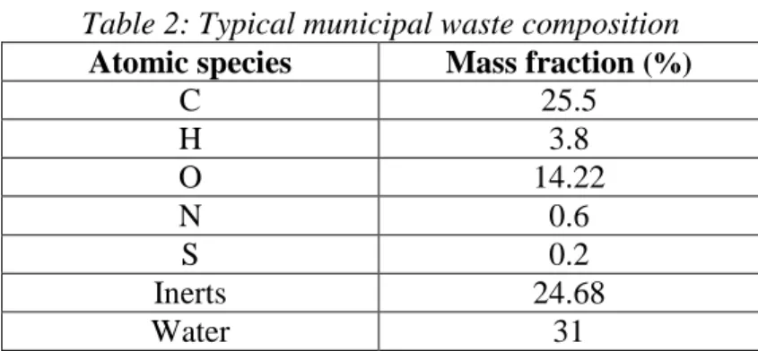
A combustion model based on the waste chemical species composition is put in place by using the general combustion equation based on waste composition from the Phyllis 2 database (2018) presented in Table 2.

Table 2: Typical municipal waste composition

Atomic species Mass fraction (%)

C 25.5 H 3.8 O 14.22 N 0.6 S 0.2 Inerts 24.68 Water 31

The general combustion equation for waste of generic chemical formula is based on Sartor et al. (2014) model validated for a large range of combustion furnaces:

( ) ( )

( )

regarding a combustion air made up mainly of nitrogen, oxygen and water (rare species like Argon are neglected). is the molar fraction of water in the fuel and represents the excess air related to the combustion. and are the respective ratios between molar fractions of nitrogen and oxygen and of water and oxygen in wet air. and are the molar coefficients of each products species. Indexes m, n, x, y and z are computed from the waste mass composition in Table 2. For instance, for carbon atoms, the index m is computed by the following equation:

[ ]

( ) The same approach is applied to compute indexes n, x, y and z. It is important to notice that mass fractions taken into account in (11) are based on the dry composition of waste without water fraction in the fuel. Molar coefficients of the products species are determined by mass conservation on the 5 different atomic species (C, H, O, N, S). Having 15 combustion products for only 5 mass conservation equations, there are 10 additional formation/dissociation equations to include in the model to obtain a determined system. These 10 formation/dissociation equations are based on the model developed by Sartor et al. (2014).

(8)

The interested reader can refer to Sartor et al. (2014) for a complete description of the chemical model of the combustion process.

The main point to focus on in this combustion model is the NOx emissions which can be an

important source of pollution in combustion processes using fuels with a non-negligible nitrogen content. In combustion processes, the main part of emissions of nitrogen oxides are NO molecules even though NO is converted into NO2 in the atmosphere. For NO formation,

there are 2 main formation mechanisms (Flagan et al., 1988), namely the thermal NO and the fuel NO. It can be noticed that there is a third formation process, the prompt NO, which can be neglected herein because this formation mechanism requires very high temperature combustion processes (Fenimore, 1971). The model from Sartor et al. (2014) is thus used in order to determine NOx emissions and compare them to European limits for a prospective

installation of a deNOx unit. 3.3. Economic assessment

In order to determine the optimal configuration to minimize costs for a prescribed heating production unit, it is necessary to define a comparison factor which illustrates a global cost related to the heating technology and type of heating distribution (centralized or decentralized). A cost of heating (COH) can be defined similarly to the levelized cost of electricity (LCOE). This cost is expressed by Eq. (12) and includes four main terms. This generic equation takes into account heat losses over the district network for centralized heating production with a factor , standing for the thermal network efficiency, including

heat losses over the network in the total energy production. [ ] ( ( ) ) (12)

CAPEX stand for the initial investment cost taking into account a depreciation rate ψ corresponding to the evolution of the initial investment cost over the lifetime of the project. C corresponds to the investment cost for the technology (€/year), Pi is the installed power of the

technology (MW) with an equivalent operating time (h). This equivalent operating time, expressed by Eq. (13), is the ratio between the total heating consumption over one year ̇ and the installed heating power .

̇ ( ) OPEX include variable costs for operation and maintenance. They are generally set up from database and can take into account electricity prices. About the electricity consumption, this cost component is important to take into account in the OPEX. For heat pumps technology, the fuel cost is free but the electricity consumed by the compressor of the heat pump system has a non-negligible part in the total COH. This cost component for a heat pump, with an average coefficient of performance , is expressed by Eq. (14).

(₎

( ) The cost of heating also includes the fuel cost taking into account an average thermal efficiency ̅ specific to each type of production. For a centralized production, electricity

CAPEX OPEX Electricity resale price + assignment of green certificates Fuel

(9)

resale prices (€/MWh) over the network as well as the assignment of a number of

green certificates at a price (€) for some technologies are also part of the total cost of

heating. In Belgium, green certificates are subsidies which are granted for the production of 1 MWhel without CO2 emissions, i.e. corresponding to CO2 savings of 456kg.

4. RESULTS

4.1. Dwellings heating requirements

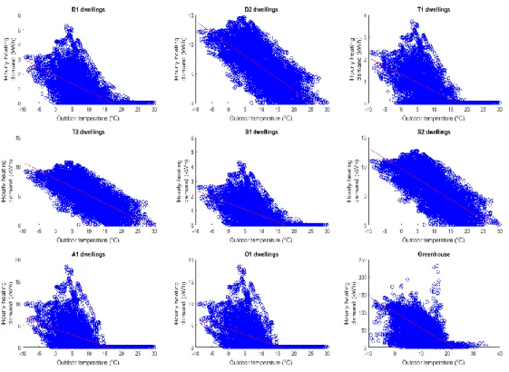
For the modelling of the district heating network, hourly heating profiles of the different dwellings have to be included in the model. Based on the mathematical models developed for the dwellings and the greenhouse (Résimont et al. & Altes-Buch et al., 2018), these heating load profiles are represented in Fig. 6.

Figure 6: Heating load profiles for the different dwellings

It can be observed from Fig. 6 that the heating consumption is very variable over the year (even for a same outdoor temperature because of inertia effects in the dwellings) such that local heating production units have to run most of the time at part-load regime. Heating demands are logically higher for poorly insulated dwellings (type 2) than for well-insulated dwellings (type 1) because of their different thermal properties. About the greenhouse heating consumption, the heating demand is important even for temperatures above 15°C. This is due to the variable set point associated to the greenhouse which determines the hourly heating demand. This set point is not totally dependent on outdoor temperatures because even for high outdoor temperatures, crops in the greenhouse can require larger heating demands (especially during nights where radiation heat losses in the greenhouse are substantial).

In order to cover heating requirements all over the year with decentralized heating units, it is necessary to install decentralized heating units with a nominal power greater than the peak heating demand over the year. These nominal powers are detailed in Table 3.

(10)

Table 3: Nominal installed heating power for each type of dwellings in the case of a decentralized heating production unit

Type of dwellings Installed power (kW)

Greenhouse 240 D1 5 D2 15 T1 5 T2 15 S1 5 S2 15 A1 20 O1 20 Total 480

From these results, a total thermal power of 480 kWth has to be installed in the dwellings and

the greenhouse for a decentralized heating production.

4.2. Cost of heating (without the allocation of green certificates)

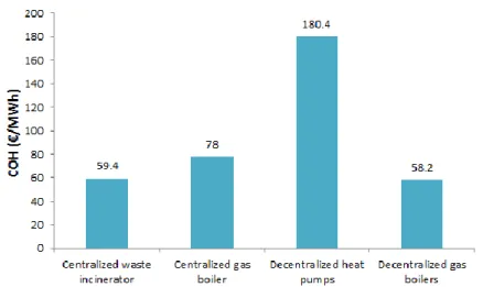
In this study, four cases including centralized and decentralized heating production units are taken into account:

1. Combination of a centralized CHP waste incinerator for base load production with backup gas boilers for peak heating production

2. Use of a centralized CHP natural gas boiler 3. Decentralized heat pumps in each dwelling 4. Decentralized natural gas boilers in each dwelling

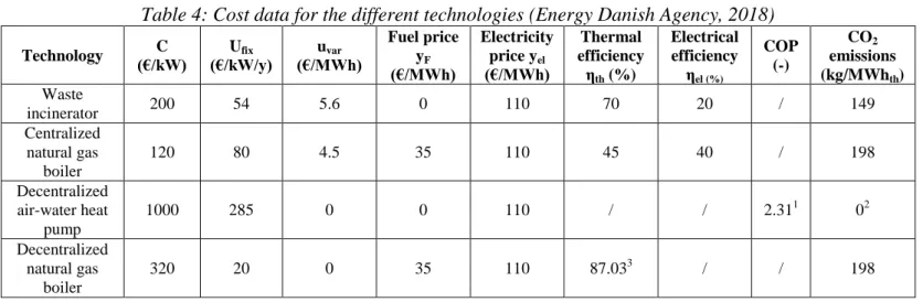
Considering a project lifetime of 20 years, a discount rate of 5% per year, a cost for pipes of 300€ per meter of pipes, a value of 65€ for each allocated green certificate and based on data from Table 4, a comparison of the cost of heating for all the scenarios mentioned above is presented in Fig. 7. The heat losses ratio 1- , which will influence the total heating

production at the power plant, is around 8.5% for respective supply and return operating temperatures of 90°C and 60°C.

Table 4: Cost data for the different technologies (Energy Danish Agency, 2018)

1_{Computed from Eq.(11)}

2

There are indirect CO2 emissions due to the electricity consumption of the heat pumps 3_{Computed from Eq.(5)}

Technology _(€/kW)C _(€/kW/y)Ufix _(€/MWh)uvar

Fuel price yF (€/MWh) Electricity price yel (€/MWh) Thermal efficiency ηth (%) Electrical efficiency ηel (%) COP (-) CO2 emissions (kg/MWhth) Waste incinerator 200 54 5.6 0 110 70 20 / 149 Centralized natural gas boiler 120 80 4.5 35 110 45 40 / 198 Decentralized air-water heat pump 1000 285 0 0 110 / / 2.311 02 Decentralized natural gas boiler 320 20 0 35 110 87.033 / / 198

(11)

Figure 7: COH for the different studied technologies without the allocation of green certificates

Two heating technologies stand out as economically profitable heating production units to minimize the cost of heating. These two technologies are a centralized heating production using waste incineration as the main heat source and a decentralized heating production unit with gas boilers in each house. It can be noticed from Fig.7 that the use of a centralized gas boiler or decentralized heat pumps in each house has a more significant cost of heating such that these technologies are excluded from an economic point of view. The choice of a centralized or a decentralized heating technology based only on an economical criterion can be filled up by an environmental analysis of the pollutants and greenhouse gases emissions for each technology. In the case of a centralized production, the pollutant model described in Section 3.2.1.can be used to determine NOx and SOx emissions due to the waste combustion

and the prospective cost of an additional deNOx unit. Moreover, based on data in Table 4, a

comparison of CO2 emissions from the different units can be established to determine the

most environmentally-friendly heating technology in terms of greenhouse gases. This analysis is achieved in the next section.

4.3. CO₂ and NO_x emissions 4.3.1. CO₂ emissions

Considering a mean value of CO2 emissions of 320 kg/MWhel for the electricity production

(Energie+, 2018) in the Belgium power station park and including the electricity consumption of the heat pumps in the CO2 balance sheet, a comparison of CO2 emissions for the four

different technologies is summarized in Fig.8.

(12)

In terms of CO2 emissions, the most suitable solution to minimize the total amount of carbon

dioxide is the heat pump technology. Despite using electricity during the compression phase of the heat pump which has an indirect impact on the CO2 emissions, there are no direct CO2

emissions with this type of technology. However, the large cost of heating of this technology excludes it as an economically optimal solution. The best compromise from an economic and environmental point of view seems therefore to be the centralized waste incineration unit which emits less CO2 than decentralized gas boiler units. It can be noticed that CO2 emissions

concerning the transport of the waste are not taken into account here in this CO2 assessment.

CO2 emissions for this heating technology are thus slightly underestimated. However,

greenhouse gases from waste transport are emitted no matter that waste are burnt or recycled by after such that there is no direct leverage on this environmental comparison.

Even though there are additional heat losses over the network for centralized heating production, waste incinerators in a district heating scenario stay thus economically and environmentally competitive compared to decentralized heating units. The main bottleneck of the waste incineration technology is the NOx pollutants emissions which have an influence on

the cost of heating due the additional cost of a deNOx unit.

4.3.2. NO_x emissions from waste incineration

From the annual heating load profile over the year of the neighborhood depicted in Fig.9, the sizing of the centralized heating plant unit can be achieved by installing a nominal power covering the maximum heating demand over the year. For the studied neighborhood, this nominal heating power is of 450 kWth such that the nominal mass flow rate related to this

heating power can be directly deduced by Eq. (15). ̇ ̇

( )

Figure 9: Annual heating consumption over the network

Pollutants emissions are based on combustion parameters summarized in Table 5 for a waste incinerator.

(13)

Table 5: Standard combustion parameters for a waste incineration.

Parameters Value

Lower Heating Value of

waste (MJ/kg) 11.71 Combustion efficiency (%) 70 Excess air e (-) 1.5 Air temperature (°C) 15 Relative humidity (%) 50

Combustion pressure (Pa) 101325 Volume of the combustion

chamber (m3) 30

Based on data from Table 5, a nominal waste mass flow rate of 138.34 kg/h is computed and is thus used in the combustion model to compute NOx emissions at a nominal point. These

emissions are compared to European legislation in terms of pollutants restricting NOx

emissions to 400 mg/Nm3 for plants with a nominal power less than 50 MWth (Directive 2010/75/UE du Parlement Européen et du conseil, 2010). These emissions standards are based on a combustion air with an O2 content of 6%. In this case study, NOx emissions are estimated

to 1511 mg/Nm3 with parameters from Table 5. This value is much higher than European standards such that a deNOx unit has to be installed. Assuming a deNOx cost around 100€/kW

of power installed (European Commission Joint Research Centre, 2017) for small-scale power plants, the additional cost related to NOx treatment for the 450 kW waste incinerator would be

of 45,000€. The cost of heating for the waste incineration technology is thus increased and is computed to 62.7€/MWh. This cost of heating is slightly larger than the cost of decentralized gas boilers in each house such that the choice of a decentralized production could be promoted from a purely economic point of view. However, the cost of heating with waste incineration could be decreased with the allocation of green certificates.

4.4. Cost of heating with the allocation of green certificates

The allocation of green certificates for the energy production with CHP heating units involves a decrease of the cost of heating. Considering a value of 65€ (value of a green certificate on the Belgian market) for each allocated green certificate, the cost of heating for the waste incineration technology with the allocation of one or two green certificates is depicted in Fig.10.

(14)

The allocation of green certificates for heating production with the waste incineration technology can decrease the cost of heating around 26.5%. With the allocation of 2 green certificates (legal limit in Belgium to allocate green certificates per MWh), the waste incineration technology becomes distinctly the most profitable solution for heating production.

5. CONCLUSION

In this paper, a generic thermal, economic and environmental model has been implemented to assess the profitability of a district heating network using a centralized heating unit compared to a decentralized heating production with production units in each house. After a description of the mathematical models used in the study to determine heating demands and pollutants emissions, a comparison of 4 scenarios including centralized and decentralized solutions has been achieved to choose the most profitable one. An economic analysis defining a cost of heating as the main key performance indicator has shown a trend about the two most profitable scenarios for a minimization of the cost of heating. These two scenarios include a centralized heating production using a waste incinerator as heating source and a decentralized one using natural gas boilers in each dwelling.

A complementary approach to determine the most environmentally-friendly solution based on greenhouse gases and pollutants emissions led to the conclusion that in terms of CO2

emissions, centralized waste incineration units enable to achieve some CO2 savings compared

to decentralized gas boiler units. The main weakness of this technology remains the NOx

emissions which are consequent due to the chemical fuel composition containing a non-negligible amount of nitrogen. Additional deNOx units have thus to be taken into account in

the economic profitability analysis of the system. Nevertheless, despite these consequent NOx

emissions, the centralization of the heating production with adequate technologies to control accurately pollutants emissions from these heating units is an additional benefit for a centralized heating production compared to a decentralized one.

Finally, taking into account the prospective allocation of green certificates with centralized CHP units, it has been shown that the cost of heating with a waste incineration unit becomes clearly more profitable than decentralized gas boilers for heating production.

NOMENCLATURE Physical quantities

c specific heat, J/(kg K)

C investment cost, €/kW

CV lumped thermal capacitance, J/K

COP Coefficient Of Performance for a heat pump, - e combustion excess air, -

G Gibbs free energy, J/kg

h enthalpy, J/kg

ki rate constant of a chemical reaction i, m3/(mol.s)

KP equilibrium constant of a chemical reaction, -

LHV Lower Heating Value, MJ/kg

̇ mass flow rate, kg/s ̇ heat flow, W

(15)

thermal resistance, K/W

s entropy, J/kg.K

tres residence time of the combustion products in the combustion chamber, s

T temperature, K or °C volume, m3

̇ volumetric flow rate, m3/s ̇ electrical production, W

xw molar fraction of water in the fuel, -

residence time of the fluid in the pipes, s

ΔT temperature difference at the primary side of the substations, K or °C Greek symbols

ratio between real and at equilibrium NO concentrations, -

β nitrogen/oxygen molar fraction in combustion air, - water/oxygen molar fraction in combustion air, -

molar coefficients of each combustion product, - percentage of conversion of fuel-N into NO, %

heat losses ratio, -

η efficiency, -

characteristic time for NO formation, s

Subscripts and superscripts comb Combustion e Equilibrium el Electrical ex Exhaust fg Flue Gases fix Fixed fl Full Load F Fuel GC Green Certificate in Indoor n Nominal pl Part-Load prim Primary out Outdoor su Supply sur Surroundings th Thermal var Variable w Water Other symbols

(16)

CHP Combined Heat and Power COH Cost Of Heating

DHN District Heating Network PLR Part Load Ratio

ACKNOWLEDGEMENTS

Financial support from FEDER Tropical Plant Factory project is duly acknowledged in the frame of this paper.

REFERENCES

UNEP – the official web site of the United Nations Environment Programme. District Energy in Cities: Unlocking the full potential of energy efficiency and renewable energy. – Available at: <http://staging.unep.org/energy/districtenergyincities>.[accessed 23.1.2018].

Rezaie B., Rosen MA, 2012. District heating and cooling: Review of technology and potential

enhancements. Applied Energy ;93:2-10.

Frederiksen S., Werner S., 2013. District heating and cooling. Studentlitteratur, Lund.

EUROPA - the official web site of the European Union. Communication From The

Commission To The European Parliament, The Council, The European Economic And Social Committee And The Committee of The Regions. An EU Strategy on Heating and Cooling –

Available at:

<https://ec.europa.eu/energy/sites/ener/files/documents/1_EN_ACT_part1_v14.pdf>.[accesse d 11.4.2018].

IEA EBC Annex 60 – the official website of the Annex 60 project of the IEA. Description of reference “Annex 60 Neighborhood Case” – Available at: <

http://www.iea-annex60.org/downloads/Annex60_2_2_ReferenceCaseStudy-v1.0.pdf> [accessed 22.10.2018]. Gabrielaitienė I, Kačianauskas B, Sunden B. 2003. Application of the Finite Element Method

for Modelling of District Heating Network. J Civ Eng Manag. 2003, 9(3), 153–62.

Résimont T., Sartor K., Dewallef P., 2018. Thermo-Economic Evaluation of a Virtual District

Heating Network Using Dynamic Simulation. ECOS 2018: Proceedings of the 31th

International Conference on Efficiency, Cost, Optimization, Simulation and Environmental Impact of Energy Systems, Guimaraes, Portugal.

Altès Buch Q., Quoilin S., Lemort V., 2018. Modeling and control of CHP generation for

greenhouse cultivation including thermal energy storage. ECOS 2018: Proceedings of the 31th

International Conference on Efficiency, Cost, Optimization, Simulation and Environmental Impact of Energy Systems, Guimaraes, Portugal.

Sartor K., Thomas D., Dewallef P., 2015. A comparative study for simulation of heat transport in large district heating network. ECOS 2015: Proceedings of the 28th International Conference on Efficiency, Cost, Optimization, Simulation and Environmental Impact of Energy Systems; Pau, France.

Van Der Heijde B., Fuchs M., Ribas C., Schweiger G., Sartor K., Basciotti D., Müller D., Nytsch-Geusen C., Wetter M., Helsen L., 2017. Dynamic equation-based thermo-hydraulic pipe model for district heating and cooling systems. Energy Convers Manage 2017, 151, 158-169.

Savola T., Keppo I., 2005. Off-design simulation and mathematical modeling of small-scale

CHP plants at part loads. Applied thermal engineering, vol.25, no 8-ç, P.1219-1232.

(17)

Ransy F., Gendebien S., Lemort V., 2017. Performances d’une mini pompe à chaleur

réversible fonctionnant sur l’air extrait : étude numérique et expérimentale. XIIIème

Colloque Interuniversitaire Franco-Québécois sur la Thermique des Systèmes. Saint-Lô, France.

Bolther A., Casari R., Fleury E., Marchio D., Millet J., 1999. Méthode de calcul des

consommations d’énergie des bâtiments climatisés « consoclim ». Ecole des Mines, Paris.

Phyllis2, database for biomass and waste, https://www.ecn.nl/phyllis2, Energy Research Centre of the Netherlands. [accessed 08.6.2018].

Sartor K., Restivo Y., Ngendakumana P., 2014. Prediction of SOx and NOx emissions from a medium size biomass boiler. Biomass and Bioenergy 2014; 65 91-100.

Fenimore CP, 1971. Formation of nitric oxide in premixed hydrocarbon flames. Proceedings of the 13th International Symposium on Combustion. Pittsburgh, P.373-380.

Hanson R.K., Salimian S., 1984. Survey of rate constants in the N/H/O system. In: Gardiner W.C. (eds). Combustion Chemistry. Springer, New York, NY.

Vermeulen I., Block C., Vandecasteele C., 2012. Estimation of fuel-nitrogen oxide emissions

from the element composition of the solid or waste fuel. Fuel Processing Technology, Vol 94,

PP.75-80.

Directive 2010/75/UE du parlement européen et du conseil du 24 novembre 2010 relative aux émissions industrielles (prévention et réduction intégrées de la pollution).

European Commission Joint Research Centre, Reference document on best available

techniques for large combustion plants - – Available at:

<https://ec.europa.eu/jrc/en/publication/eur-scientific-and-technical-research-reports/best-available-techniques-bat-reference-document-large-combustion-plants-industrial>[accessed 13.4.2018].

Energy Danish Agency. Technology Data for Energy Plants – Available at: <

https://ens.dk/sites/ens.dk/files/Analyser/technology_data_catalogue_for_el_and_dh_-_aug_2016_upd_oct18.pdf >.[accessed 05.11.2018].

Energie+ - Outil d’aide à la décision en efficacité énergétique des bâtiments tertiaires – Available at : <https://www.energieplus-lesite.be/>[accessed 08.6.2018].