Efficient Algorithms for Large-Scale Topology Discovery
Benoit Donnet
∗Universit´e Pierre & Marie Curie Laboratoire LiP6–CNRS
Philippe Raoult
Universit´e Pierre & Marie CurieLaboratoire LiP6–CNRS
Timur Friedman
Universit´e Pierre & Marie Curie Laboratoire LiP6–CNRS
Mark Crovella
Boston University Computer Science DepartmentABSTRACT
There is a growing interest in discovery of internet topology at the interface level. A new generation of highly distributed measurement systems is currently being deployed. Unfortu-nately, the research community has not examined the prob-lem of how to perform such measurements efficiently and in a network-friendly manner. In this paper we make two con-tributions toward that end. First, we show that standard topology discovery methods (e.g., skitter) are quite ineffi-cient, repeatedly probing the same interfaces. This is a con-cern, because when scaled up, such methods will generate so much traffic that they will begin to resemble DDoS attacks. We measure two kinds of redundancy in probing (intra- and inter-monitor) and show that both kinds are important. We show that straightforward approaches to addressing these two kinds of redundancy must take opposite tacks, and are thus fundamentally in conflict. Our second contribution is to propose and evaluate Doubletree, an algorithm that re-duces both types of redundancy simultaneously on routers and end systems. The key ideas are to exploit the tree-like structure of routes to and from a single point in order to guide when to stop probing, and to probe each path by starting near its midpoint. Our results show that Doubletree can reduce both types of measurement load on the network dramatically, while permitting discovery of nearly the same set of nodes and links.
∗The authors are participants in the traceroute@home
project.This work was supported by: the RNRT project Metropolis, NSF grants ANI-9986397 and CCR-0325701, a SATIN European Doctoral Research Foundation grant, the e-Next European Network of Excellence, and LiP6 2004 project funds. This work was performed while Mr. Crovella was at LiP6, with support from the CNRS and Sprint Labs.
Permission to make digital or hard copies of all or part of this work for personal or classroom use is granted without fee provided that copies are not made or distributed for profit or commercial advantage and that copies bear this notice and the full citation on the first page. To copy otherwise, to republish, to post on servers or to redistribute to lists, requires prior specific permission and/or a fee.
SIGMETRICS’05, June 6–10, 2005, Banff, Alberta, Canada.
Copyright 2005 ACM 1-59593-022-1/05/0006 ...$5.00.
Categories and Subject Descriptors
C.2.1 [Network Architecture and Design]: Network topology
General Terms
Algorithms, Measurements
Keywords
network topology, traceroutes, cooperative systems
1. INTRODUCTION
Systems for active measurements in the internet are un-dergoing a radical shift. Whereas the present generation of systems operates on largely dedicated hosts, numbering be-tween 20 and 200, a new generation of easily downloadable measurement software means that infrastructures based on thousands of hosts could spring up literally overnight. Un-less carefully controlled, these new systems have the poten-tial to impose a heavy load on parts of the network that are being measured. They also have the potential to raise alarms, as their traffic can easily resemble a distributed de-nial of service (DDoS) attack. This paper examines the problem, and proposes and evaluates an algorithm for con-trolling one of the most common forms of active measure-ment: traceroute [30].
There is a number of systems active today that aim to elicit the internet topology at the IP interface level. The most extensive tracing system, Caida’s skitter [16], uses 24 monitors, each targeting on the order of one million desti-nations. Some other well known systems, such as the Ripe NCC’s TTM service [14] and the NLanr AMP [22], have larger numbers of monitors (between one- and two-hundred), and conduct traces in a full mesh, but avoid tracing to out-side destinations.
The uses of the raw data from these traces are numerous. From a scientific point of view, the results underlie efforts to model the network [2, 6, 12, 13, 21, 28]. From an en-gineering standpoint, the results inform a wide variety of protocol development choices, such as multicast and overlay construction [25].
However, recent studies have shown that reliance upon a relatively small number of monitors to generate a graph of the internet can introduce unwanted biases. For instance, the work by Faloutsos et al. [12] found that the distribution of router degrees follows a power law. That work was based
upon an internet topology collected from just twelve trace-route hosts by Pansiot and Grad [23]. However, Lakhina et al. [20] showed that, in simulations of a network in which the degree distribution does not at all follow a power law, trace-routes conducted from a small number of monitors can tend to induce a subgraph in which the node degree distribution does follow a power law. Clauset and Moore [8] have since demonstrated analytically that such a phenomenon is to be expected for the specific case of the Erd¨os-R´enyi random graphs [11].
Removing spatial bias is not the only reason to employ measurement systems that use a larger number of monitors. With more monitors to probe the same space, each one can take a smaller portion and probe it more frequently. Net-work dynamics that might be missed by smaller systems can more readily be captured by the larger ones while keeping the workload per monitor constant.
The idea of releasing easily deployable measurement soft-ware is not new. To the best of our knowledge, the idea of incorporating a traceroute monitor into a screen saver was first discussed in a paper by Cheswick et al. [7] from the year 2000 (they attribute the suggestion to J¨org Nonnen-macher). Since that time, a number of measurement tools have been released to the public in the form of screen savers or daemons. Grenouille [1], which is used for measuring available bandwidth in DSL connections, was perhaps the first, and appears to be the most widely adopted. More re-cently, we have seen the introduction of NETI@home [26], a passive measurement tool inspired by the distributed sig-nal asig-nalysis tool, SETI@home [3]. In the summer of 2004, the first tracerouting tool of this type was made available: DIMES [24] conducts traceroutes and pings from, at the time of this writing, 639 sites in 49 countries.
Given that much large scale network mapping is on the way, contemplating such a measurement system demands at-tention to efficiency, in order to avoid generating undesirable network load. Unfortunately, this issue has not been yet suc-cessfully tackled by the research community. As Cheswick, Burch and Branigan note, such a system “would have to be engineered very carefully to avoid abuse” [7, Sec. 7]. Trace-routes emanating from a large number of monitors and con-verging on selected targets can easily appear to be a DDoS attack. Whether or not it triggers alarms, it clearly is not de-sirable for a measurement system to consume undue network resources. A traceroute@home system, as we label this class of applications, must work hard to avoid sampling router interfaces and traversing links multiple times, and to avoid multiple pings of end systems.
This lack of consideration of efficiency for internet mon-itoring system is in contrast with the work performed on efficient monitoring of networks that are in a single admin-istrative domain (see for instance, Bejerano and Rastogi’s work [4]). However, the problem is completely different. An administrator knows their entire network topology in ad-vance, and can freely choose where to place their monitors. Neither of these assumptions hold for monitoring the in-ternet with highly distributed monitors. Since the existing literature is based upon these assumptions, we need to look elsewhere for solutions.
Our first contribution, in this paper, is to evaluate the extent to which classical topology discovery systems involve duplicated effort. By classical topology discovery, we mean those systems, such as skitter, tracing from a small number
of monitors to a large set of common destinations, such as skitter. Duplicated effort in such systems takes two forms: measurements made by an individual monitor that replicate its own work, and measurements made by multiple mon-itors that replicate each other’s work. We term the first intra-monitor redundancy and the second inter-monitor re-dundancy.
Using skitter data from August 2004, we quantify both kinds of redundancy. We show that intra-monitor redun-dancy is high close to each monitor. This fact is not sur-prising given the tree-like structure (or cone, as Broido and claffy describe it in [6]) of routes emanating from a single monitor. However, the degree of such redundancy is quite elevated: some interfaces are visited once for each destina-tion probed (which could be hundreds of thousands of times per day in a large-scale system). Further, with respect to inter-monitor redundancy, we find that most interfaces are visited by all monitors, especially when close to destinations. This latter form of redundancy is also potentially quite large, since this would be expected to grow linearly with the num-ber of monitors in future large-scale measurement systems.
Our analysis of the nature of redundant probing suggests more efficient algorithms for topology discovery. In partic-ular, our second contribution is to propose and evaluate an algorithm called Doubletree. We show that Doubletree can dramatically reduce the impact on routers and final desti-nations by reducing redundant probing, while maintaining high coverage in terms of interface and link discovery. Dou-bletree is particularly effective at removing the worst cases of highly redundant probing that would be expected to raise alarms.
Doubletree takes advantage of the tree-like structure of routes, either emanating from a single source to multiple destinations or routes converging from multiple sources to a single destination, to avoid duplication of effort. Unfor-tunately, general strategies for reducing these two kinds of redundancy are in conflict. On the one hand, intra-monitor redundancy is reduced by starting probing far from the mon-itor, and working backward along the tree-like structure that is rooted at that monitor. Once an interface is encountered that has already been discovered by the monitor, probing stops. On the other hand, inter-monitor redundancy is re-duced by probing forwards towards a destination until en-countering a previously-seen interface.
We show a means of balancing these conflicting strate-gies in Doubletree. In Doubletree, probing starts at a dis-tance that is intermediate between monitor and destination. We demonstrate methods for choosing this distance, and we then evaluate the resulting performance of Doubletree. De-spite the challenge inherent in reducing both forms of redun-dancy simultaneously, we show that probing via Doubletree can reduce measurement load by approximately 76% while maintaining interface and link coverage above 90%.
The remainder of this paper is organized as follow: Sec. 2 evaluates the extent of redundancy in classical topology trac-ing systems. Sec. 3 describes and evaluates the Doubletree algorithm. Finally, Sec. 4 concludes this paper and intro-duces directions for future work.
2. REDUNDANCY
In this section we quantify and analyze the extensive mea-surement redundancy that can be found in a classical topol-ogy discovery system.
2.1 Methodology
Our study is based on skitter data from August 1stthrough
3rd, 2004. This data set was generated by 24 monitors
lo-cated in the United States, Canada, the United Kingdom, France, Sweden, the Netherlands, Japan, and New Zealand. The monitors share a common destination set of 971,080 IPv4 addresses. Each monitor cycles through the destina-tion set at its own rate, taking typically three days to com-plete a cycle. For the purpose of our studies, in order to reduce computing time to a manageable level, we worked from a limited destination set of 50,000, randomly chosen from the original set.
Visits to host and router interfaces are the metric by which we evaluate redundancy. We consider an interface to have been visited if its IP address returned by the router appears, at least, at one of the hops in a traceroute. Though it would be of interest to calculate the load at the host and router level, rather than at the individual interface level, we make no attempt to disambiguate interfaces in order to obtain a router-level information. The alias resolution techniques de-scribed by Pansiot and Grad [23], by Govindan and Tang-munarunkit [15], for Mercator, and applied in the iffinder tool from Caida [19], would require active probing beyond the skitter data, preferably at the same time that the skitter data is collected. The methods used by Spring et al. [27], in Rocketfuel, and by Teixeira et al. [29], apply to routers in the network core, and are untested in stub networks. Despite these limitations, we believe that the load on individual in-terfaces is a useful measure. As Broido and claffy note [6], “interfaces are individual devices, with their own individual processors, memory, buses, and failure modes. It is reason-able to view them as nodes with their own connections.”
How do we account for skitter visits to router and host interfaces? Like many standard traceroute implementations, skitter sends three probe packets for each hop count. An IP address appears thus in a traceroute result if it replies, at least, to one of the three probes sent (but it may also response two or three times). If none of the three probes are returned, the hop is recorded as non-responding.
Even if an IP address is returned for a given hop count, it might not be valid. Due to the presence of poorly con-figured routers along traceroute paths, skitter occasionally records anomalies such as private IP addresses that are not globally routable. We account for invalid hops as if they were non-responding hops. The addresses that we consider as invalid are a subset of the special-use IPv4 addresses de-scribed in RFC 3330 [17]. Specifically, we eliminate visits to the private IP address blocks 10.0.0.0/8, 172.16.0.0/12, and 192.168.0.0/16. We also remove the loopback address block 127.0.0.0/8. In our data set, we find 4,435 differ-ent special addresses, more precisely 4,434 are private dresses and only one is a loopback address. Special ad-dresses cover around 3% of the entire considered adad-dresses set. Though there were no visits in the data to the follow-ing address blocks, they too would be considered invalid: the “this network” block 0.0.0.0/8, the 6to4 relay anycast address block 192.88.99.0/24, the benchmark testing block 198.18.0.0/15, the multicast address block 224.0.0.0/4, and
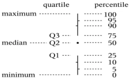
Figure 1: Quantiles key
the reserved address block formerly known as the Class E addresses, 240.0.0.0/4, which includes the lan broadcast ad-dress, 255.255.255.255.
We evaluate the redundancy at two levels. One is the individual level of a single monitor, considered in isolation from the rest of the system. This intra-monitor redundancy is measured by the number of times the same monitor visits an interface. The other, global, level considers the system as an ensemble of monitors. This inter-monitor redundancy is measured by the number of monitors that visit a given in-terface, counting only once each monitor that has non-zero intra-monitor redundancy for that interface. By separat-ing the two levels, we separate the problem of redundancy into two problems that can be treated somewhat separately. Each monitor can act on its own to reduce its intra-monitor redundancy, but cooperation between monitors is required to reduce inter-monitor redundancy.
2.2 Description of the Plots
In this section, we plot interface redundancy distributions. Since these distributions are generally skewed, quantile plots give us a better sense of the data than would plots of the mean and variance. There are several possible ways to cal-culate quantiles. We calcal-culate them in the manner described by Jain [18, p. 194], which is: rounding to the nearest inte-ger value to obtain the index of the element in question, and using the lower integer if the quantile falls exactly halfway between two integers.
Fig. 1 provides a key to reading the quantile plots found in Figs. 2 and 3 and figures found later in the paper. A dot marks the median (the 2ndquartile, or 50thpercentile).
The vertical line below the dot delineates the range from the minimum to the 1stquartile, and leaves a space from the 1st
to the 2nd quartile. The space above the dot runs from the
2ndto the 3rdquartile, and the line above that extends from the 3rd quartile to the maximum. Small tick bars to either
side of the lines mark some additional percentiles: bars to the left for the 10th and 90th, and bars to the right for the 5th and 95th.
In the case of highly skewed distributions, or distributions drawn from small amounts of data, the vertical lines or the spaces between them might not appear. For instance, if there are tick marks but no vertical line above the dot, this means that the 3rd quartile is identical to the maximum
value.
In the figures, each quantile plot sits directly above an accompanying bar chart that indicates the quantity of data upon which the quantiles were based. For each hop count, the bar chart displays the number of interfaces at that dis-tance. For these bar charts, a log scale is used on the vertical
axis. This allows us to identify quantiles that are based upon very few interfaces (fewer than twenty, for instance), and so for which the values risk being somewhat arbitrary.
In addition, each plot has a separate bar to the right, la-beled “all”, that shows the quantiles for all interfaces taken together (upper part of the plot) and the amount of discov-ered interfaces (lower part of the plot).
2.3 Intra-monitor Redundancy
Intra-monitor redundancy occurs in the context of the tree-like graph that is generated when all traceroutes origi-nate at a single point. Since there are fewer interfaces closer to the monitor, those interfaces will tend to be visited more frequently. In the extreme case, if there is a single gateway router between the monitor and the rest of the internet, the single IP address of the outgoing interface belonging to that router should show up in every one of the traceroutes.
We measure intra-monitor redundancy by considering all traceroutes from the monitor to the shared destinations, whether there be problems with a traceroute such as ille-gal addresses, as described in Sec. 2.1, or not.
Having calculated the intra-monitor redundancy for each interface, we organize the results by the distance of the in-terfaces from the monitor. We measure distance by hop count. Since the same interface can appear at a number of different hop counts from a monitor, for instance if routes change between traceroutes, we arbitrarily attribute to each interface the hop count at which it was first visited. This process yields, for each hop count, a set of interfaces that we sort by number of visits. We then plot, hop by hop, the redundancy distribution for interfaces at each hop count.
2.3.1 Results
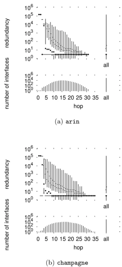
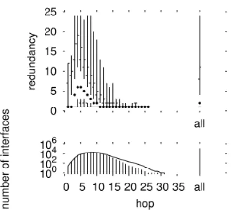
Fig. 2 shows intra-monitor redundancy quantile distribu-tions for two representative skitter monitors: arin and cham-pagne.
Looking first at the histograms for interface counts (lower half of each plot), we see that these data are consistent with distributions typically seen in such cases. If we look at a plot on a linear scale (not shown here) these distributions dis-play the familiar bell-shaped curve typical of internet inter-face distance distributions. The distribution for champagne (shown in Fig. 2(b)) is fairly typical of all monitors1. It rep-resents the 92,354 unique IP addresses discovered by that monitor. This value is shown as a separate bar to the right of the histogram, labeled “all”. The interface distances are distributed with a mean at 17 hops corresponding to a peak of 9,135 interfaces that are visited at that distance.
The quantile plots show the nature of the intra-monitor redundancy problem. Looking first to the bar at the right hand of each chart, we can see that the distributions are highly skewed. The lower quantile and the median interface have a redundancy of one, as evidenced by the lack of a gap between the dot and the line representing the bottom quarter of values. However, for a very small portion of the interfaces there is a very high redundancy. The maximum redundancy in each case is 150,000 — equal to the number of destinations multiplied by the three probes sent at each hop.
Looking at how the redundancy varies by distance, we see that the problem is worse the closer one is to the
moni-1A full version of this paper, including more plots, is
avail-able online [10] 106 104 102 100 all 35 30 25 20 15 10 5 0
number of interfaces hop
106 105 104 103 102 101 100 all redundancy (a) arin 106 104 102 100 all 35 30 25 20 15 10 5 0
number of interfaces hop
106 105 104 103 102 101 100 all redundancy (b) champagne
Figure 2: Skitter intra-monitor redundancy
tor. This is what we expect given the tree-like structure of routing from a monitor, but here we see how serious the phe-nomenon is from a quantitative standpoint. For the first two hops from each monitor, the median redundancy is 150,000. A look at the histograms shows that there are very few inter-faces at these distances. Just one interface for arin, and two (2ndhop) or three (3rdhop) for champagne. These interfaces
are only visited three times, as represented by the presence of the 5th and 10th percentile marks (since there are only
two data points, the lower values point is represented by the entire lower quarter of values on the plot).
Beyond three hops, the median redundancy drops rapidly. By the eleventh hop, in both cases, the median is below ten. However, the distributions remain highly skewed. Even fifteen hops out, some interfaces experience a redundancy on the order of several hundred visits. With small variations, these patterns are repeated for each of the monitors.
From the point of view of planning a measurement sys-tem, the extreme values are the most worrisome. It is clear that there is significant duplicated effort, but it is especially concentrated in selected areas. The problem is most severe on the first few interfaces, but even interfaces many hops out receive hundreds or thousands of repeat visits. Beyond
Destinations Responding 59.7% Not responding 40.3% Probes Interface discovery 10.9% Invalid addresses 1.5% No response 0.7% Redundant 86.6%
Table 1: Additional statistics for champagne
the danger of triggering alarms, there is a simple question of measurement efficiency. Resources devoted to reprobing the same interfaces would be better saved, or reallocated to more fruitful probing tasks.
Table 1 presents additional statistics for champagne. The first part of the table indicates the portion of destinations that respond and the portion that do not respond. Fully 40.3% of the traceroutes do not terminate with a destination response. The second part of the table describes redundancy in terms of probes sent, rather than from an interface’s per-spective. Only 10.9% of probes serve to discover a new in-terface. (Note: in the intra-monitor context, an interface is considered to be new if that particular monitor has not pre-viously visited it.) An additional 2.2% of probes hit invalid addresses, as defined in Sec. 2.1, or do not result in a re-sponse. This leaves 86.6% of the probes that are redundant in the sense that they visit interfaces that the monitor has already discovered. The statistics in this table are typical of the statistics for every one of the 24 monitors.
2.4 Inter-monitor Redundancy
Inter-monitor redundancy occurs when multiple monitors visit the same interface. The degree of such redundancy is of keen interest to us when increasing the number of monitors by several orders of magnitude is envisaged.
We calculate the monitor redundancy for each inter-face by counting the number of monitors that have visited it. A monitor can be counted at most once towards an inter-face’s inter-monitor redundancy, even if it has visited that interface multiple times. For a given interface, the redun-dancy is calculated just once with respect to the entirety of the monitors: it does not vary from monitor to monitor as does intra-monitor redundancy. However, what does vary depending upon the monitor is whether the particular in-terface is seen, and at what distance. In order to attribute a single distance to an interface, a distance that does not depend upon the perspective of a single monitor but that nonetheless has meaning when examining the effects of dis-tance on redundancy, we attribute the minimum disdis-tance at which an interface has been seen among all the monitors.
106 104 102 100 all 35 30 25 20 15 10 5 0
number of interfaces hop 0 5 10 15 20 25 all redundancy
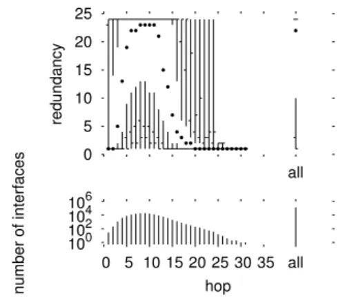
Figure 3: Skitter inter-monitor redundancy
2.4.1 Results
Fig. 3 shows inter-monitor redundancy for the skitter data. The distribution of interfaces by hop count differs from the intra-monitor case due to the difference in how we account for distances. The mean is closer to the traceroute source (9 hops), corresponding to the peak of 19,742 interfaces that are visited at that distance.
The redundancy distribution also has a very different as-pect. Considering, first, the redundancy over all of the in-terfaces (at the far right of the plot), we see that the me-dian interface is visited by nearly all 24 monitors, which is a subject of great concern. The distribution is also skewed, though the effect is less dramatic since the vertical axis is a linear scale, with only 24 possible values.
We also see a very different distribution by distance. Inter-faces that are very close in to a monitor, at one or two hops, have a median inter-monitor redundancy of one. The same is true of interfaces that are far from all monitors, at dis-tances over 20, though there are very few of these. What is especially notable is that interfaces at intermediate distances (5 to 13) tend to be visited by almost all of the monitors. Though their distances are in the middle of the distribution, this does not mean that the interfaces themselves are in the middle of the network. Many of these interfaces are in fact destinations. Recall that every destination is targeted by every host.
3. ALGORITHM
In this section, we present the Doubletree algorithm, our method for probing the network in a friendly manner while discovering nearly all the interfaces and links that a classical tracerouting approach would discover.
Sec. 3.1 describes how Doubletree works. Sec. 3.2 dis-cusses the results of varying the single parameter of this algorithm. Sec. 3.3 shows the extent of intra- and inter-monitor redundancy reduction when using the algorithm. Finally, Sec. 3.4 describes some features about how Double-tree could be implemented in reality.
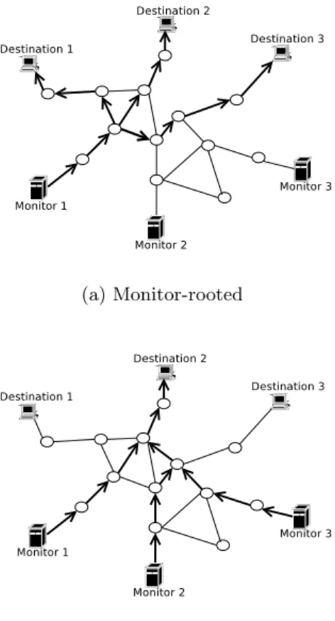
(a) Monitor-rooted
(b) Destination-rooted
Figure 4: Tree-like routing structures
3.1 Description
Doubletree takes advantage of the tree-like structure of routes in the internet. Routes lead out from a monitor to-wards multiple destinations in a tree-like way, as shown in Fig. 4(a), and the manner in which routes converge towards a destination from multiple monitors is similarly tree-like, as shown in Fig. 4(b). The tree is an idealisation of the struc-ture encountered in practice. In reality, paths can separate and reconverge. Loops can arise. But a tree may be a good enough first approximation on which to base a redundancy reduction technique.
A probing algorithm can reduce its redundancy by track-ing its progress through a tree, as it probes from the direc-tion of the leaves towards the root. So long as it is probing in a previously unknown part of the tree, it continues to probe. But once it encounters a node that is already known to belong to the tree, it stops. The idea being that the re-mainder of the path to the root must already be known. In reality, there is only a likelihood and not a certainty that the remainder of the path is known. The redundancy saved by not reprobing the same paths to the root may nonetheless be worth the loss in coverage that results from not prob-ing the occasional different path. This is especially true if lower redundancy allows more frequent probing, increas-ing the number of network snapshots that can be captured per unit time. A series of snapshots might capture route changes, mitigating the effect of missing nodes or links due
to routing changes in the midst of any individual snapshot. The gains from more frequent snapshots are a subject for future work.
Doubletree uses both the monitor-rooted and the destination-rooted trees. When probing backwards from the destina-tions towards the monitor, it applies a stopping rule based upon the monitor-rooted tree. The goal in this case is to reduce intra-monitor redundancy. When probing forwards, the stopping rule is based upon the destination-rooted tree, with the goal being to reduce inter-monitor redundancy. There is an inherent tension between the two goals.
Suppose the algorithm were to start probing only far from each monitor. Probing would necessarily be backwards. In this case, the destination-based trees cannot be used to re-duce redundancy. A monitor might discover, with desti-nation d at hop h, an interface that another monitor also discovered when probing with destination d. However this does not inform the monitor as to whether the interface at hop h− 1 is likely to have been discovered as well. So it is not clear how to reduce inter-monitor redundancy when conducting backwards probing. Further, exclusive use of backwards probing would mean that destinations will be hit each time, increasing the risk of probing appearing to be a DDoS attack.
Similarly, when conducting forwards probing (of the clas-sic traceroute sort), it is not clear how intra-monitor redun-dancy can be avoided. Paths close to the monitor will tend to be probed and reprobed, for lack of knowledge of where the path to a given destination might diverge from the paths already seen.
In order to reduce both inter- and intra-monitor redun-dancy, Doubletree starts probing at what is hoped to be an intermediate point. For each monitor, there is an initial hop count h. Probing proceeds forwards from h, to h + 1, h + 2, and so forth, applying the stopping rule based on the destination-rooted tree. Then it probes backwards from h− 1 to h − 2, h − 3, etc., using the monitor-based tree stopping rule. In the special case where there is no response at distance h, the distance is halved, and halved again until there is a reply, and probing continues forwards and back-wards from that point.
Rather than maintaining detailed information on tree struc-tures, it is sufficient for the stopping rules to make use of sets of (interface, root) pairs, the root being the root of the tree in question, either monitor-rooted or destination-rooted. We call these sets stop sets. A Doubletree monitor takes into account one of two different stop sets, depending on the direction in which it is probing. When probing back-wards, it uses a stop set B , called the backwards tracing stop set, or more concisely, the local stop set. As backwards probing concerns the monitor-rooted tree, the item root of the pairs is implicit (i.e. it is the monitor itself) and it is thus not necessary to record it in the local stop set. There-fore, the local stop set can be more efficiently stored as a set of interfaces. When probing backwards from a destina-tion d, encountering an interface in B causes the monitor to stop and move on to the next destination. Each monitor also receives another stop set, F , called the forwards tracing stop set, or more concisely, the global stop set, that con-tains (interface, destination) pairs. When probing forwards towards destination d and encountering an interface i, for-wards probing stops if (i, d)∈ F . Communication between monitors is needed in order to share this second stop set.
Algorithm 1 Doubletree
Require: F , the global stop set received by this monitor. Ensure: F updated with all (interface,destination) pairs
discovered by this monitor. 1: procedure Doubletree(h, D)
2: B← ∅ . Local stop set
3: for all d∈ D do . Destinations
4: h← AdaptHValue(h) . Initial hop
5: TraceForwards(h, d)
6: TraceBackwards(h− 1, d)
7: end for
8: end procedure
9: procedure AdaptHValue(h)
10: while¬response(vh)∧ h 6= 1 do . vh the interface
discovered at h hops 11: h←h 2 . h an integer 12: end while 13: return h 14: end procedure 15: procedure TraceForwards(i, d) 16: while vi6= d ∧ (vi, d) /∈ F ∧ ¬halt() do 17: F← FS(vi, d) 18: i + + 19: end while 20: end procedure 21: procedure TraceBackwards(i, d) 22: while i> 1 ∧ vi∈ B ∧ ¬halt() do/ 23: B← BSvi 24: F← FS(vi, d) 25: i− − 26: end while 27: end procedure
Only one aspect of Doubletree has been suggested in prior literature. Govindan and Tangmunarunkit [15] employ back-wards probing with a stopping rule in the Mercator system, in order to reduce intra-monitor redundancy. However, no results have been published regarding the efficacy of this ap-proach. Nor have the effects on inter-monitor redundancy been considered, or the tension between reducing the two types of redundancy (for instance, Mercator tries to start probing at the destination, or as close to it as possible, which, as we have seen, is highly deleterious to inter-monitor redundancy). Nor has any prior work suggested a manner in which to exploit the tree-like structure of routes that con-verge on a destination. Finally, no prior work has suggested cooperation among monitors.
Algorithm 1 is a formal definition of the Doubletree algo-rithm. It assumes that the following two functions are de-fined. The response() procedure returns true if an interface replies to at least one of the probes that were sent. halt() is a primitive that checks if the probing must be stopped for different reasons: a loop is detected or a gap (five successive non-responding nodes) is discovered.
This algorithm has only one tunable value: the initial hop count h. In the remainder of this section, we explain how to set this value in terms of a parameter that we call p.
We wish for each monitor to be able to determine a
0.00 0.10 0.20 0.30 0.40 0.50 0.60 0.70 0.80 0.90 1.00 0 5 10 15 20 25 30 35 40 cumulative mass path length
Figure 5: Lengths of paths from monitor apan-jp
sonable value for h: one that is far enough from the monitor to avoid excess intra-monitor redundancy, yet not so far as to generate too much inter-monitor redundancy. Since each monitor will be positioned differently with respect to the internet, what is a reasonable hop count for one monitor might not be reasonable for another. We thus base our rule for choosing h on the distribution of path lengths as seen in-dividually from the perspective of each monitor. The general idea is to start probing at a distance that is rich in inter-faces, but that is not so far as to exacerbate inter-monitor redundancy.
Based upon our intra-monitor redundancy studies, dis-cussed above, we would expect an initial hop distance of five or more from the typical monitor to be fairly rich in interfaces. However, we also know that this is a distance at which inter-monitor redundancy can become a problem. We are especially concerned about inter-monitor redundancy at destinations, because this is what is most likely to look like a DDoS attack.
One parameter that a monitor can estimate without much effort is its probability of hitting a responding destination at any particular hop count h. For instance, Fig. 5 shows the cumulative mass plot of path lengths from monitor apan-jp. If apan-jp considers that a 0.1 probability of hitting a re-sponding destination on the first probe is reasonable, it must chose h = 10. The shape of this curve is very similar for each of the 24 skitter monitors, but the horizontal position of the curve can vary by a number of hops from monitor to monitor. So if we are to fix the probability, p, of hit-ting a responding destination on the first probe, there will be different values h for each monitor, but that value will correspond to a similar level of incursion into the network across the board.
We have chosen p to be the single independent parameter that must be tuned to guide Doubletree. In the following section, we study the effect of varying p on the tension be-tween inter- and intra-monitor redundancy, and the overall interface and link coverage that probing with Doubletree obtains.
3.2 Tuning the Parameter p
This section discusses the effect of varying p. Sec. 3.2.1 de-scribes our experimental methodology, and Sec. 3.2.2 presents the results.
3.2.1 Methodology
In order to test the effects of the parameter p on both redundancy and coverage, we implement Doubletree in a simulator. We examine the following values for p: between 0 (i.e., forwards probing only) and 0.2, we increment p in steps of 0.01. From 0.2 to 1 (i.e., backwards probing in all cases when the destination replies to the first probe), we increment p in steps of 0.1. As will be shown, the concentration of values close to 0 allows us to trace the greater variation of behavior in this area.
To validate our results, we run the simulator using the skitter data from early August 2004. We assume that Dou-bletree is running on the skitter monitors, during the same period of time that the skitter data represents, and imple-menting the same baseline probing technique described in Sec. 2.1, of probing up to three times at a given hop dis-tance. The difference in the application of Doubletree lies in the order in which Doubletree probes the hops, and the application of Doubletree’s stopping rules.
A single experiment uses traceroutes from all 24 monitors to a common set of 50,000 destinations chosen at random. Each data point represents the mean value over fifteen runs of the experiment, each run using a different set of 50,000 destinations randomly generated. No destination is used more than once over the fifteen runs. We determine 95% confidence intervals for the mean based, since the sample size is relatively small, on the Student t distribution. These intervals are typically, though not in all cases, too tight to appear on the plots.
Doubletree requires communication of the global stop set from one monitor to another. We therefore choose a random order for the monitors and simulate the running of Double-tree on each one in turn. Each monitor adds to the global set (interface, destination) pairs that it encounters, and passes it to the subsequent monitor. This is a simplified scenario compared to the way in which a fully operational coopera-tive topology discovery protocol might function, which is to say with all of the monitors probing and communicating in parallel (see Sec. 3.4). However, we feel that the scenario allows greater realism in the study of intra-monitor redun-dancy. The typical monitor in a large, highly distributed infrastructure will begin its probing in a situation in which much of the topology has already been discovered by other monitors. The closest we can get to simulating the experi-ence of such a monitor is by studying what happens to the last in our random sequence of monitors. All Doubletree intra-monitor redundancy results are for the last monitor in the sequence. (Inter-monitor redundancy, on the other hand, is monitor independent.)
3.2.2 Results
Since the value p has a direct effect on the redundancy of destination interfaces, we initially look at the effect of p separately on destination redundancy and on router inter-face redundancy. We are most concerned about destination redundancy because of its tendency to appear like a DDoS attack, and we are concerned in particular with the inter-monitor redundancy on these destinations, because a vari-ety of sources is a prime indicator of such an attack. The right-side vertical axis of Fig. 6 displays destination redun-dancy. With regards router interface redundancy, which is displayed on the left-side vertical axis, we are concerned with overall load, and so we consider a combined intra- and
300 350 400 450 500 550 600 0 0.2 0.4 0.6 0.8 1 0 5 10 15 20 25
router gross redundancy destination redundancy
p
interface destination
Figure 6: Doubletree redundancy, 95th percentile.
Inter-monitor redundancy on destinations, gross re-dundancy on router interfaces.
0 0.2 0.4 0.6 0.8 1 0 0.2 0.4 0.6 0.8 1
coverage in comparison to skitter
p
nodes links
Figure 7: Link and nodes coverage in comparison to classic probing
monitor redundancy measure that we call gross redundancy, that counts the total number of visits to an interface. For both destinations and router interfaces, we are concerned with the extreme values, so we consider the 95th percentile. As expected the 95thpercentile inter-monitor redundancy
on destinations increases with p. Values increase until p = 0.5, at which point they plateau at 24. The point p = 0.5 is, by definition, the point at which the probe sent to a dis-tance h hits a destination in 50% of the cases. Doubletree allows a reduction in 95th percentile inter-monitor redun-dancy when compared to classical probing for lower values of p. The maximum reduction is 84% when p = 0, implying pure forward probing.
As opposed to destination redundancy, the 95thpercentile gross router interface redundancy decreases with p. The 95th
percentile for the internal interface gross redundancy using the classical approach is 1340. Doubletree thus allows a reduction between 59.6% (p = 0) and 72.6% (p = 1).
This preliminary analysis suggests that Doubletree should employ a low value for p, certainly below 0.5, in order to re-duce inter-monitor redundancy on destinations. This is a very different approach than that taken by Mercator, which attempts to hit a destination every time. On the other hand, too low a value will have a negative impact on router inter-faces. We now examine other evidence that will bear on our choice of p.
105 106 107 108
0 0.2 0.4 0.6 0.8 1
number of probes sent
p
min probes for interface discovery min probes for link discovery nb probes for skitter
Figure 8: Number of probes sent
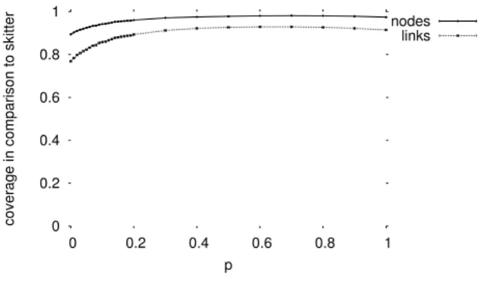
Fig. 7 illustrates the effects of p on the node and link cov-erage percentage in comparison to classic probing. As we can see, the coverage increases with p but a small decrease is noticed for values of p greater than 0.7. The maximum coverage is reached approximatively when p = 0.7: Dou-bletree discovers 92.9% of links and 98.1% of nodes. The minimum of coverage appears when p = 0: 76.8% of links and 89.3% of nodes. However, link coverage grows rapidly for p values between 0 and 0.4. After that point, a kind of plateau is reached, before a small decrease.
Fig. 7 shows that the information (i.e. links and nodes) discovery of our algorithm is relatively high, especially for non zero values of p.
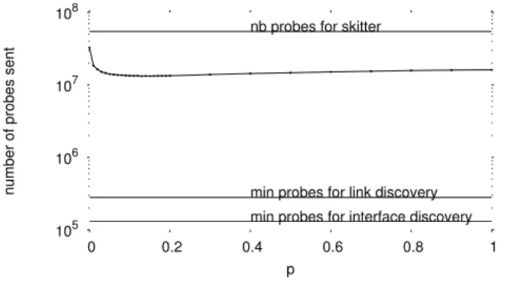
Fig. 8 shows the effects of p on the number of probes sent. The horizontal axis indicates the value for p. The vertical axis represents the number of probes sent. If we consider an ideal system in which each probe sent visits a new interface (i.e., there is no redundancy), the number of probes sent to discover all the interfaces will be 131,476 (i.e., the mean number of different interfaces in the data set). This bound is shown by the lowest horizontal line. If, on the other hand, the ideal system is also able to discover links without any link redundancy, but incurring the necessary interface re-dundancy, then it should send, on average, 279,799 probes. This is the second horizontal line shown in the plot. At the other extreme, if our system works like skitter, it sends 54,634,841 probes. This is represented by the highest hori-zontal line. With Doubletree, the number of probes needed varies between 32,652,958 (i.e., a reduction of 40.3% in com-parison to the classical approach) and 13,230,106 (i.e., a re-duction of 75.8% in comparison to the classical approach). This minimum is reached when p = 0.15.
The results presented in this section are important in the case of a highly distributed measurement tool. They demon-strate that it is possible to probe in a network friendly man-ner while maintaining a very high level of topological infor-mation gathered by monitors.
The results in this section permit us to identify a range of values for which a good compromise between redundancy reduction and high level of coverage is possible. For the remainder of this paper, we consider p values in the range from 0.05 to 0.2. 106 104 102 100 all 35 30 25 20 15 10 5 0
number of interfaces hop
106 105 104 103 102 101 100 all redundancy
Figure 9: Intra-monitor redundancy for the
champagne monitor with p = 0.05.
3.3 Redundancy Reduction
In this section, we study the effects of Doubletree on the intra- and inter-monitor redundancy compared to re-dundancy in skitter, as presented in Sec. 2. Sec. 3.3.1 de-scribes our methodology. Sec. 3.3.2 presents the intra- and Sec. 3.3.3 the inter-monitor redundancy reduction.
3.3.1 Methodology
We use the simulator to study the effects of Doubletree on intra- and inter-monitor redundancy. Again, for comparison reasons, we use the same data set as in Sec. 2.
The plots are presented in the same way as in Sec. 2. However, the lower part of the graphs, the histograms, con-tain additional information. The bars are now enveloped by a curve. This curve indicates, for each hop, the quantity of nodes discovered while using the classical method. The bars themselves describe the number of nodes discovered us-ing Doubletree. Therefore, the space between the bars and the curve represents the quantity of nodes exploration with Doubletree misses.
In Sec. 3.2, we identify a range of p values for which re-dundancy is relatively low and coverage is relatively high. We run simulations for p = 0.05, p = 0.1, p = 0.15 and p = 0.2 and study the effects on inter- and intra-monitor redundancy reduction. Having found the the differences be-tween the results for these values of p to be small, we present only the results for p = 0.05 in this section.
3.3.2 Intra-monitor
Fig. 9 shows intra-monitor redundancy when using Dou-bletree with p = 0.05 for a representative monitor: champagne.
First of all, we note that, using Doubletree, champagne is able to elicit 97% of the interfaces in comparison to the classical method.
Looking to the right part of the plot first, we note that the median redundancy is 3. It is somewhat higher than for the classical method. As in the classical approach, for a very small number of interfaces there is a high redundancy. With Doubletree the maximum is only 750. Compared to the 150,000 in the classical approach, there is a reduction of 99.5%.
Looking now at how the redundancy varies by distance, we note a strong reduction for Doubletree with respect to
106 104 102 100 all 35 30 25 20 15 10 5 0
number of interfaces hop 0 5 10 15 20 25 all redundancy
Figure 10: Inter-monitor redundancy with p = 0.05.
classical approaches for the median values close to the mon-itor. (see, for comparison, Fig. 2(b)). Somewhat further out, the reduction is somewhat less pronounced Finally, we note that high quantiles for hops far from the source have somewhat higher values than for the classical method. The strong drop in redundancy close to the monitor thus comes at the expense of some increased redundancy further out. The overall effect is one of smoothing the load.
3.3.3 Inter-monitor
Fig. 10 shows inter-monitor redundancy when using Dou-bletree with p = 0.05.
We first analyse the lower part of the graph. The distri-bution of hop counts for interfaces shows that most of the undiscovered interfaces are far from the source. As most of these nodes are only visited by a single monitor (see Fig. 3), due to the nature of the global stop set and the stop rule, the risk of missing them is very high. Probably, with a higher value for p, probing with Doubletree would have elicited them. However, this solution would raise the redundancy for destinations, as explained in Sec. 3.2.2. Those undiscov-ered nodes are, in a certain sense, the price to pay to reduce the redundancy. This demonstrates the inherent tension in the topology discovery problem.
If we compare Fig. 10 with Fig. 3, we can see that the redundancy is strongly reduced. The highest value for the median is only 6. For the classical method, it is equal to 23. Furthermore, the highest quantiles between hop 4 and 13 are more dissipated.
Finally, the right part of the graph, called all, indicates that the median value is 2. If we compare with Fig. 3, where the median equals 22, we note that Doubletree allows a very strong reduction in inter-monitor redundancy.
3.4 Deploying Doubletree
Until now, we have considered a simplified application of Doubletree, where each monitor probes the destination list in turn and, at the end of the process, sends its global stop set to the next monitor. This round robin process is not nec-essarily what one might wish in reality because it is too re-strictive and too slow. Further, for our simulations, we had, a priori, full knowledge of path lengths, making possible an accurate choice for each monitor of the h value correspond-ing to the chosen p. In practice, such knowledge would need to be learned. In this section, we aim to explain the way
Doubletree can be implemented in reality. We also indicate how to improve the communication between monitors.
The round robin process of exploring path is not suitable. It is preferable that all monitors perform their exploration in parallel. However, how would one manage the global stop set if it were being updated by all the monitors at the same time, with the attendant risk of re-exploring paths?
An easy way to tackle this problem is to divide the des-tinations list into subsets. Each subset is investigated by a different monitor. When a monitor finishes probing its destination subset, it sends its global stop set back to a cen-tralized server. The cencen-tralized server merges all the global stop sets and distributes it to all monitors. Next, the mon-itors exchange their destinations subsets. This process is performed until each monitor has probed each destination subset.
An operational system implementing Doubletree cannot choose the value h as a function of p a priori, as we did in our experiments. It can be, however, easily compute h in the beginning by using an iterative process before probing the destinations. It simply needs to ping a certain number (high enough) of destinations to get path lengths, compute the cumulative mass distribution based on this sample and then, decide the h value according to a value of p belonging to the range [0.05, 0.2]. This method implies a small additional load on destinations. A trade-off must be made between the accuracy of the parameter h and the load on destinations.
One possible obstacle to successful deployment of Double-tree concerns the communication overhead from sharing the global stop set among monitors. Tracing from 24 monitors to just 50,000 destinations with p = 0.05 produces a set of 2.7 million (interface, destination) pairs. As pairs of IPv4 addresses are 64 bits long, an uncompressed stop set based on these parameters requires 20.6MB.
A way to reduce this communication overhead is to use Bloom filters [5] to implement the global stop set. A Bloom filter summarizes information concerning a set in a bit vec-tor that can then be tested for set membership. An empty Bloom filter is a vector of all zeroes. A key is registered in the filter by hashing it to a position in the vector and setting the bit at that position to one. Multiple hash functions may be used, setting several bits set to one. Membership of a key in the filter is tested by checking if all hash positions are set to one. A Bloom filter will never falsely return a negative result for set membership. It might, however, return a false positive. For a given number of keys, the larger the Bloom filter, the less likely is a false positive. The number of hash functions also plays a role.
In an extension [9] of the work described here, we show that, when p = 0.05, using a bit vector of size 107 and five hash functions allow nearly the same coverage level as a list implementation of the global stop set while reducing only slightly the redundancy on both destinations and internal interfaces and yielding a compression factor of 17.3.
4. CONCLUSION
In this paper, we quantify the amount of redundancy in classical internet topology discovery approaches by taking into account the perspective from the single monitor (intra-monitor) and that of the entire system (inter-(intra-monitor). In the intra-monitor case, we find that interfaces close to the monitor suffer from a high number of repeat visits. We also show that only 10.9% of probes serve to discover a new
interface. Concerning inter-monitor redundancy, we see that a large portion of interfaces are visited by all monitors.
In order to scale up classical approaches such as skit-ter, we have proposed Doubletree, an algorithm that sig-nificantly reduces the duplication of effort while discovering nearly the same set of nodes and links. Doubletree simulta-neously meets the conflicting demands of reducing intra- and inter-monitor redundancy. We describe how to tune a single parameter for Doubletree in order to obtain an acceptable trade-off between redundancy and coverage.
For a range of p values, Doubletree is able to reduce mea-surement load by approximately 76% while maintaining in-terface and link coverage above 90%.
Doubletree introduces communication between monitors. We pointed out that the communication cost required may be a brake to the wide deployment of Doubletree. To address the problem of bandwidth consumption, we introduce an extension [9] to this work in which we propose to encode this communication through the use of Bloom filters.
Our extension to this work also considers the fact that a probing technique that starts probing at a hop h far from the monitor has a non zero probability p of hitting a destination with its first probe. This has serious consequences when scaling up the number of monitors. Indeed, the average impact on destinations will grow linearly as a function of m, the number of monitors. As m increases, the risk that probing will appear to be a DDoS attack will grow. We started to investigate techniques for dividing up the monitor set and the destination set into subsets that we call clusters [9]. For future work, we aim to investigate a process where this affectation will be based on topological criteria.
This implies, however, to have a topology with a larger number of monitors. To achieve that, we are starting to implement Doubletree in order to test it on a middle-size infrastructure (on the order of a few hundred monitors).
Finally, we plan to improve Doubletree in order to allow topology discovery at the IP interface level guided by BGP. We believe that a Doubletree monitor can profitably make use of higher level information, such as the AS topology.
Acknowledgments
Without the skitter data provided by kc claffy and her team at CAIDA, this research would not have been possible. They also furnished much useful feedback. Marc Giusti and his team at the Centre de Calcul MEDICIS, Laboratoire STIX, Ecole Polytechnique, offered us access to their computing cluster, allowing faster and easier simulations. Finally, we are indebted to our colleagues in the Networks and Perfor-mance Analysis group at LiP6, headed by Serge Fdida, and to our partners in the traceroute@home project, Jos´e Ig-nacio Alvarez-Hamelin, Alain Barrat, Matthieu Latapy and Alessandro Vespignani, for their support and advice.
5. REFERENCES
[1] A. Schmitt et al. La m´et´eo du net, ongoing service. See: http://www.grenouille.com/.
[2] S. Agarwal, L. Subramanian, J. Rexford, and R. Katz. Characterizing the internet hierarchy from multiple vantage points. In Proc. IEEE INFOCOM, June 2002. [3] D. P. Anderson, J. Cobb, E. Korpela, M. Lebofsky,
and D. Werthimer. SETI@home: An experiment in public-resource computing. Communications of the
ACM, 45(11):56–61, Nov. 2002. See also the SETI@home project:
http://setiathome.ssl.berkeley.edu/.
[4] Y. Bejerano and R. Rastogi. Robust monitoring of link delays and faults in IP networks. In Proc. IEEE Infocom, Mar. 2003.
[5] B. H. Bloom. Space/time trade-offs in hash coding with allowable errors. Communications of the ACM, 13(7):422–426, 1970.
[6] A. Broido and k. claffy. Internet topology: Connectivity of IP graphs. In Proc. SPIE
International Symposium on Convergence of IT and Communication, 2001.
[7] B. Cheswick, H. Burch, and S. Branigan. Mapping and visualizing the internet. In Proc. USENIX Annual Technical Conference, 2000.
[8] A. Clauset and C. Moore. Traceroute sampling makes random graphs appear to have power law degree distributions. arXiv:cond-mat/0312674 v3 8 Feb. 2004. [9] B. Donnet, T. Friedman, and M. Crovella. Improved
algorithms for network topology discovery. In Proc. of Passive and Active Measurement Workshop (PAM), Mar. 2005.
[10] B. Donnet, P. Raoult, T. Friedman, and M. Crovella. Efficient algorithms for large-scale topology discovery. 2004. arXiv:cs.NI/0411013. See also the
traceroute@home project:
http://www.tracerouteathome.net/.
[11] P. Erd¨os and A. R´enyi. On the evolution of random graphs. Publ. Math. Inst. Hung. Acad. Sci., 5:17–61, 1960.
[12] M. Faloutsos, P. Faloutsos, and C. Faloutsos. On power-law relationships of the internet topology. In Proc. ACM SIGCOMM, 1999.
[13] L. Gao. On inferring autonomous system relationships in the internet. In Proc. IEEE Global Internet Symposium, Nov. 2000.
[14] F. Georgatos, F. Gruber, D. Karrenberg, M. Santcroos, A. Susanj, H. Uijterwaal, and R. Wilhelm. Providing active measurements as a regular service for ISPs. In Proc. PAM, 2001. See also the RIPE NCC TTM service:
http://www.ripe.net/test-traffic/.
[15] R. Govindan and H. Tangmunarunkit. Heuristics for internet map discovery. In Proc. IEEE Infocom, 2000. [16] B. Huffaker, D. Plummer, D. Moore, and k. claffy.
Topology discovery by active probing. In Symposium on Applications and the Internet, Jan. 2002.
[17] IANA. Special-use IPv4 addresses. RFC 3330, Internet Engineering Task Force, Sep. 2002.
[18] R. K. Jain. The Art of Computer Systems Performance Analysis. John Wiley, 1991.
[19] K. Keys. iffinder. A tool for mapping interfaces to routers. See http:
//www.caida.org/tools/measurement/iffinder/. [20] A. Lakhina, J. Byers, M. Crovella, and P. Xie.
Sampling biases in IP topology measurements. In Proc. IEEE Infocom, 2003.
[21] D. Magoni and J. J. Pansiot. Analysis of the autonomous system network topology. ACM SIGCOMM Computer Communication Review, 31(3):26 – 37, Jul. 2001.
[22] A. McGregor, H.-W. Braun, and J. Brown. The NLANR network analysis infrastructure. IEEE Communications Magazine, 38(5):122–128, May 2000. See also the NLANR AMP project:
http://watt.nlanr.net/.
[23] J. J. Pansiot and D. Grad. On routes and multicast trees in the internet. ACM SIGCOMM Computer Communication Review, 28(1):41–50, Jan. 1998. [24] Y. Shavitt. DIMES. Distributed Internet
Measurements & Simulations. See: http://www.netdimes.org/.
[25] R. Siamwalla, R. Sharma, and S. Keshav. Discovering internet topology. Technical report, Cornell University, July 1998.
[26] C. R. Simpson, Jr. and G. F. Riley. NETI@home: A distributed approach to collecting end-to-end network performance measurements. In Proc. PAM, 2004. See also the NETI@home project:
http://www.neti.gatech.edu/.
[27] N. Spring, R. Mahajan, and D. Wetherall. Measuring ISP topologies with Rocketfuel. In Proc. ACM SIGCOMM, 2002.
[28] H. Tangmunarunkit, J. Doyle, R. Govindan, S. Jamin, and S. Shenker. Does AS size determine degree in AS topology? In ACM SIGCOMM Computer
Communication Review, volume 31, Oct. 2001. [29] R. Teixeira, K. Marzullo, S. Savage, and G. Voelker.
In search of path diversity in ISP networks. In Proc. Internet Measurement Conference (IMC), 2003. [30] V. Jacobsen et al. traceroute. man page, UNIX, 1989.
See source code:
ftp://ftp.ee.lbl.gov/traceroute.tar.gz, and NANOG traceroute source code: