Y. Muraki1,67, C. Han2,68,∗, D.P. Bennett3,67,70,∗, D. Suzuki4,67, L.A.G. Monard5,68, R. Street6,69, U.G. Jorgensen7,71, P. Kundurthy8, J. Skowron9,68, A.C. Becker8, M.D. Albrow10,70, P. Fouqu´e11,70, D. Heyrovsk´y12, R.K. Barry13, J.-P. Beaulieu14,70,
D.D. Wellnitz15, I.A. Bond16,67, T. Sumi4,17,67, S. Dong18,68, B.S. Gaudi9,68, D.M. Bramich19,69, M. Dominik20,21,69,71,
and
F. Abe4, C.S. Botzler22, M. Freeman22, A. Fukui4, K. Furusawa4, F. Hayashi4, J.B. Hearnshaw10, S. Hosaka4, Y. Itow4, K. Kamiya4, A.V. Korpela23, P.M. Kilmartin24, W. Lin16, C.H. Ling16, S. Makita4, K. Masuda4, Y. Matsubara4, N. Miyake4, K. Nishimoto4,
K. Ohnishi25, Y.C. Perrott22, N.J. Rattenbury26, To. Saito27, L. Skuljan16, D.J. Sullivan23, W.L. Sweatman16, P.J. Tristram24, K. Wada1, P.C.M. Yock22,
(The MOA Collaboration)
G.W. Christie28, D.L. DePoy29, E. Gorbikov30, A. Gould9, S. Kaspi30, C.-U. Lee31, F. Mallia32, D. Maoz30, J. McCormick33, D. Moorhouse34, T. Natusch28, B.-G. Park31,
R.W. Pogge9, D. Polishook35, A. Shporer30, G. Thornley34, J.C. Yee9, (The µFUN Collaboration)
A. Allan36, P. Browne20,71, K. Horne20, N. Kains19, C. Snodgrass37,38,71, I. Steele39, Y. Tsapras6,40,
(The RoboNet Collaboration)
V. Batista14, C.S. Bennett41, S. Brillant37, J.A.R. Caldwell42, A. Cassan14, A. Cole43, R. Corrales14, Ch. Coutures14, S. Dieters43, D. Dominis Prester44, J. Donatowicz45,
J. Greenhill43, D. Kubas14,37, J.-B. Marquette14, R. Martin46, J Menzies47, K.C. Sahu48, I. Waldman49, A. Williams46 M. Zub50,
(The PLANET Collaboration)
H. Bourhrous51, Y. Matsuoka52, T. Nagayama52, N. Oi53, Z. Randriamanakoto47, (IRSF Observers)
V. Bozza54,55, M.J. Burgdorf56,57, S. Calchi Novati54, S. Dreizler58, F. Finet59, M. Glitrup6, K. Harpsøe7, T.C. Hinse7,31, M. Hundertmark58, C. Liebig20, G. Maier50,
L. Mancini54,61, M. Mathiasen7, S. Rahvar62, D. Ricci59, G. Scarpetta54,55, J. Skottfelt7, J. Surdej59, J. Southworth63, J. Wambsganss50, F. Zimmer50,
(The MiNDSTEp Consortium)
A. Udalski64, R. Poleski64, L. Wyrzykowski64,65, K. Ulaczyk64, M.K. Szyma´nski64, M. Kubiak64, G. Pietrzy´nski64,66, I. Soszy´nski64
(The OGLE Collaboration)
1
Department of Physics, Konan University, Nishiokamoto 8-9-1, Kobe 658-8501, Japan
∗
To whom correspondence should be addressed; E-mail: bennett@nd.edu, cheongho@chungbuk.ac.kr
2
Department of Physics, Chungbuk National University, 410 Seongbong-Rho, Hungduk-Gu, Chongju 371-763, Korea
3Department of Physics, 225 Nieuwland Science Hall, University of Notre Dame, Notre Dame, IN 46556, USA
4
Solar-Terrestrial Environment Laboratory, Nagoya University, Nagoya, 464-8601, Japan
5Bronberg Observatory, Centre for Backyard Astrophysics, Pretoria, South Africa
6
Las Cumbres Observatory Global Telescope Network, 6740 Cortona Dr., Suite 102, Goleta, CA 93117, USA
7
Niels Bohr Institute and Centre for Stars and Planet Formation, Juliane Mariesvej 30, 2100 Copenhagen, Denmark
8Astronomy Department, University of Washington, Seattle, WA 98195
9
Department of Astronomy, Ohio State University, 140 West 18th Avenue, Columbus, OH 43210, USA
10University of Canterbury, Department of Physics and Astronomy, Private Bag 4800, Christchurch 8020, New
Zealand
11
IRAP, CNRS, Universit´e de Toulouse, 14 avenue Edouard Belin, 31400 Toulouse, France
12Institute of Theoretical Physics, Charles University, V Holeˇsoviˇck´ach 2, 18000 Prague, Czech Republic
13
Goddard Space Flight Center, Greenbelt, MD 20771, USA
14
Institut d’Astrophysique de Paris, F-75014, Paris, France
15University of Maryland, College Park, MD 20742, USA
16
Institute for Information and Mathematical Sciences, Massey University, Private Bag 102-904, Auckland 1330, New Zealand
17Department of Earth and Space Science, Osaka University, 1-1 Machikaneyama-cho, Toyonaka, Osaka 560-0043,
Japan
18
Sagan Fellow; Institute for Advanced Study, Einstein Drive, Princeton, NJ 08540, USA
19
European Southern Observatory, Karl-Schwarzschild-Straße 2, 85748 Garching bei M¨unchen, Germany
20
SUPA, University of St Andrews, School of Physics & Astronomy,North Haugh, St Andrews, KY16 9SS, UK
21
Royal Society University Research Fellow
22Department of Physics, University of Auckland, Private Bag 92-019, Auckland 1001, New Zealand
23
School of Chemical and Physical Sciences, Victoria University, Wellington, New Zealand
24Mt. John University Observatory, P.O. Box 56, Lake Tekapo 8770, New Zealand
25
Nagano National College of Technology, Nagano 381-8550, Japan
26Jodrell Bank Observatory, The University of Manchester, Macclesfield, Cheshire SK11 9DL, UK
27
Tokyo Metropolitan College of Aeronautics, Tokyo 116-8523, Japan
28
Auckland Observatory, P.O. Box 24-180, Auckland, New Zealand
30
School of Physics and Astronomy, Raymond and Beverley Sackler Faculty of Exact Sciences, Tel-Aviv University, Tel Aviv 69978, Israel
31Korea Astronomy and Space Science Institute, 776 Daedukdae-ro, Yuseong-gu 305-348 Daejeon, Korea
32
Campo Catino Austral Observatory, San Pedro de Atacama, Chile
33
Farm Cove Observatory, 2/24 Rapallo Place, Pakuranga, Auckland 1706, New Zealand
34
Kumeu Observatory, Kumeu, New Zealand
35
Benoziyo Center for Astrophysics, Weizmann Institute of Science
36School of Physics, University of Exeter, Stocker Road, Exeter, EX4 4QL, UK
37
European Southern Observatory, Casilla 19001, Vitacura 19, Santiago, Chile
38Max-Planck-Institut fr Sonnensystemforschung, Katlenburg-Lindau, Germany
39
Astrophysics Research Institute, Liverpool John Moores University, Twelve Quays House, Egerton Wharf, Birken-head CH41 1LD, UK
40
Astronomy Unit, School of Mathematical Sciences, Queen Mary, University of London, London E1 4NS
41
Department of Physics, Massachusetts Institute of Technology, 77 Mass. Ave., Cambridge, MA 02139
42
McDonald Observatory, 16120 St Hwy Spur 78 #2, Fort Davis, TX 79734
43University of Tasmania, School of Mathematics and Physics, Private Bag 37, Hobart, TAS 7001, Australia
44
Department of Physics, University of Rijeka, Omladinska 14, 51000 Rijeka, Croatia
45Technische Universitaet Wien, Wieder Hauptst. 8-10, A-1040 Wienna, Austria
46
Perth Observatory, Walnut Road, Bickley, Perth 6076, WA, Australia
47South African Astronomical Observatory, P.O. Box 9 Observatory 7925, South Africa
48
Space Telescope Science Institute, 3700 San Martin Drive, Baltimore, MD 21218, USA
49
University College London, Dept. of Physics and Astronomy, Gower Street, London WC1E 6BT, UK
50Astronomisches Rechen-Institut, Zentrum f¨ur Astronomie der Universit¨at Heidelberg, M¨onchhofstrasse 12-14,
69120 Heidelberg, Germany
51
Department of Mathematics and Applied Mathematics, University of Cape Town, Rondebosch 7701, Cape Town, South Africa
52Graduate School of Science, Nagoya University, Furo- cho, Chikusa-ku, Nagoya 464-8602, Japan
53
Department of Astronomical Science, The Graduate University for Advanced Studies (Sokendai), Mitaka, Tokyo 181-8588, Japan
54
Department of Physics, University of Salerno, Via Ponte Don Melillo, 84084 Fisciano (SA), Italy
55Istituto Nazionale di Fisica Nucleare, Sezione di Napoli, Italy
56
SOFIA Science Center, NASA Ames Research Center, Mail Stop N211-3, Moffett Field CA 94035, USA
57Deutsches SOFIA Institut, Universitaet Stuttgart, Pfaffenwaldring 31, 70569 Stuttgart, Germany
58
Institut fur Astrophysik, Georg-August-Universitat, Friedrich-Hund-Platz 1, 37077 Gottingen, Germany
ABSTRACT
We present the discovery and mass measurement of the cold, low-mass planet MOA-2009-BLG-266Lb, made with the gravitational microlensing method. This planet has a mass of mp = 10.4 ± 1.7M⊕ and orbits a star of mass M? = 0.56 ± 0.09M at a semi-major axis of a = 3.2+1.9−0.5AU and an orbital period of P = 7.6+7.7−1.5yrs. The planet and host star mass measurements are enabled by the measurement of the microlensing parallax effect, which is seen primarily in the light curve distortion due to the orbital motion of the Earth. But, the analysis also demonstrates the capability to measure microlensing parallax with the Deep Impact (or EPOXI) spacecraft in a Heliocentric orbit. The planet mass and orbital distance are similar to predictions for the critical core mass needed to accrete a substantial gaseous envelope, and thus may indicate that this planet is a “failed” gas giant. This and future microlensing detections will test planet formation theory predictions regarding the prevalence and masses of such planets. Subject headings: gravitational lensing: micro, planetary systems
1. Introduction
In the leading core accretion planet formation model (Lissauer 1993), a key role is played by the “snow line”, where the proto-planetary disk becomes cold enough for ices to condense. The timescale for agglomeration of small bodies into protoplanets is shortest just beyond the snow line, because this is where the surface density of solid material is highest. The largest protoplanets in
60
Department of Physics & Astronomy, Aarhus University, Ny Munkegade 120, 8000 Arhus C, Denmark
61
Max Planck Institute for Astronomy, K¨onigstuhl 17, 69117 Heidelberg, Germany
62 Department of Physics, Sharif University of Technology, and School of Astronomy, IPM, 19395-5531, Tehran,
Iran
63
Astrophysics Group, Keele University, Staffordshire, ST5 5BG, United Kingdom
64Warsaw University Observatory, Al. Ujazdowskie 4, 00-478 Warszawa, Poland
65
Institute of Astronomy, Univ. of Cambridge, Madingley Road, Cambridge CB3 0HA, UK
66
Universidad de Concepci´on, Departamento de Astronomia, Casilla 160–C, Concepci´on, Chile
67
Microlensing Observations in Astrophysics (MOA) Collaboration
68
Microlensing Follow Up Network (µFUN) Collaboration
69RoboNet Collaboration
70
Probing Lensing Anomalies Network (PLANET) Collaboration
these regions are expected to quickly reach a mass of ∼ 10M⊕ by accumulating the majority of the solid material in their vicinity. They then slowly accrete a gaseous envelope of hydrogen and helium. The envelope can no longer maintain hydrostatic equilibrium when it reaches the mass of the core, so it collapses, starting a rapid gas accretion phase that leads to a massive giant planet. The hydrostatic accretion phase is predicted to have a much longer duration than the other two phases of solid accretion and rapid gas accretion (Pollack et al. 1996). This has several possible implications, including a higher frequency of low-mass, rocky/icy planets than gas giants, a feature in the final mass function of planets near the critical core mass of ∼ 10 M⊕, a relative paucity of planets with masses of 10 − 100 M⊕ (Ida & Lin 2004), and the formation of very few gas giants orbiting low-mass hosts (Laughlin et al. 2004), where the gas disks are expected to dissipate before the critical core mass is reached.
These predictions follow from general physical considerations, but they also rely upon a number of simplifying assumptions that make the calculations tractable. So, they could be incorrect. For example, recent work suggests that uncertainties in the initial surface density of solids in the protoplanetary disk, grain opacities in protoplanetary atmospheres, and the size distribution of accreting planetesimals can radically alter the timescales of these various phases and thus the resulting distribution of final planet masses (Rafikov 2011; Hubickyj et al. 2005; Movshovitz & Podolak 2008). Therefore, the measurement of the mass function of planets down to below the predicted critical core mass will provide important constraints on the physics of planet formation. Attempts to test core accretion theory predictions with the mass distribution of the ∼ 500 detected exoplanets and the ∼ 1200 candidate exoplanets found by the Kepler mission (Borucki et al. 2011) have met with varied success. Radial velocity detections confirm the prediction that massive gas giants should be rare around low-mass stars (Johnson et al. 2010), but the prediction that 10 − 100 M⊕ planets should be rare in short period orbits is contradicted by the data (Howard et al. 2010). Kepler finds a large population of planets at ∼ 2.5 R⊕ in short period orbits, which is consistent with a result from the radial velocity planet detection method (Howard et al. 2010). This might be considered a confirmation of the core accretion theory prediction that ∼ 10 M⊕ “failed gas giant core” planets should be common, but in fact all of the low-mass planets found by radial velocity and transit methods have been well interior to the snow line, where these “failed core” planets are thought to form. It is possible that the exoplanet mass (or radius) function is quite different outside the snow line due to such processes as sorting by mass through migration (Ward 1997) and photo-evaporation of gaseous envelopes (Baraffe et al. 2005). Thus, a study of the exoplanet mass function beyond the snow line should provide a sharper test of the core accretion theory.
The gravitational microlensing method (Mao & Paczy´nski 1991; Bennett 2008; Gaudi 2010) has demonstrated sensitivity extending down to planets of mass < 10M⊕ in orbits beyond the snow line (Bennett & Rhie 1996; Beaulieu et al. 2006; Bennett et al. 2008). Thus it can provide a complementary probe of the physics of planet formation for planets that have migrated little from their putative birth sites. A statistical analysis of some of the first microlensing discoveries (Gould
et al. 2010) indicates that cold, Saturn-mass planets beyond the snow line are more common than gas giants found in closer orbits with the Doppler radial velocity method (Cumming et al. 2008). Another microlensing study (Sumi et al. 2010) of the mass function slope showed that planets of ∼ 10M⊕ are even more common than these cold Saturns, in general agreement with the core accretion theory prediction for “failed gas giant cores” (Kennedy & Kenyon 2008; Thommes et al. 2008).
A well sampled planetary microlensing light curve provides a direct determination of the planet:star mass ratio, but not the individual masses of planet and host star. Furthermore, planets found by microlensing typically have distant, low-mass host stars, so their faintness makes them difficult to characterize. While finite source effects in the light curve do constrain a combination of the mass and distance, it has often been necessary to estimate the planet and host masses and distance with a Bayesian analysis (Beaulieu et al. 2006) based on a Galactic model and prior as-sumptions about the exoplanet distribution. When the masses of planetary microlenses and their host stars can be measured, they will provide tighter constraints on planet formation theory.
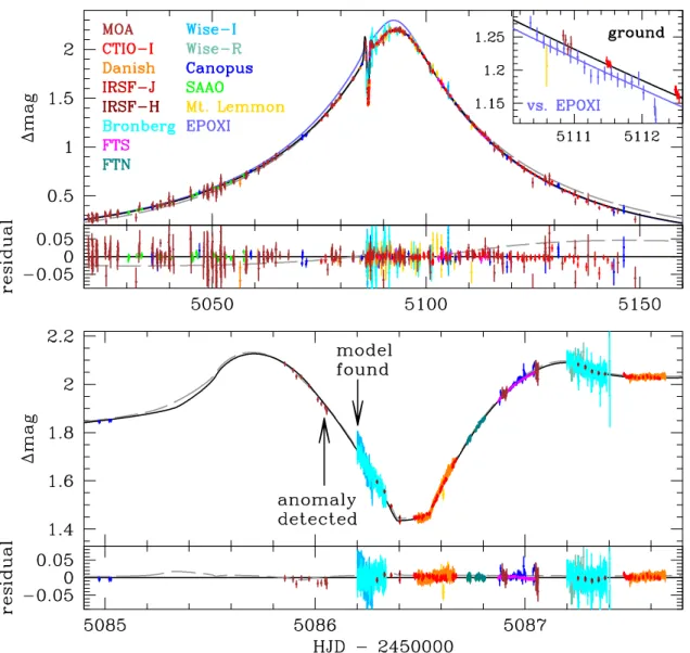
Here, we present the first example of a mass measurement for a cold, low-mass planet discovered by microlensing, which has a mass very similar to the expected critical mass for gas accretion. The light curve of microlensing event MOA-2009-BLG-266 exhibits a planetary signal due to a companion with a mass ratio of ∼ 6×10⁻⁵(see Figure 1). The light curve also reveals a microlensing parallax signal due to the orbital motion of the Earth (Gould 1992; Alcock et al. 1995). When combined with the information from the finite size of the source during the planetary perturbation, this allows one to work out the complete geometry of the microlensing event (Gould 1992), yielding a measurement of the host and planet masses. This has been done previously at this level of precision only for the giant planets in the system OGLE-2006-BLG-109L (Gaudi et al. 2008; Bennett et al. 2010). In addition, observations from the EPOXI spacecraft in a heliocentric orbit corroborate the mass measurement for MOA-2009-BLG-266Lb, and demonstrate the potential of obtaining masses for planetary events that are too brief for a parallax measurement due to the Earth’s orbit.
Our observations are described in Section 2, and Section 3 details our data reduction proce-dures. Section 4 presents a detailed discussion of the source star properties, and we discuss the determination of the properties of the planetary system in Section 5. Finally, we discuss some of the implications of this discovery in Section 6.
2. Observations
The microlensing event MOA-2009-BLG-266 [(RA, DEC) = (17h 48m 05.95s, −35◦ 000 19.4800) and (l, b) = (−4.9◦, −3.6◦)] was discovered on 1 June 2009 by the Microlensing Observations in Astrophysics (MOA) collaboration MOA-II 1.8m survey telescope at Mt. John University Ob-servatory in New Zealand. The Probing Lensing Anomalies NETwork (PLANET), Microlensing Follow-Up Network (µFUN) and Microlensing Network for the Detection of Small Terrestrial
Ex-oplanets (MiNDSTEp) teams followed some of the early part of the light curve. The wide field of view (2.2 deg2) of the MOA-II survey telescope allows MOA to monitor the Galactic bulge with a high enough cadence to discover planetary signals in any of the 500-600 microlensing events they discover every year, and this has resulted in the discovery of several exoplanets (Sumi et al. 2010; Bennett et al. 2008). On 11 September 2009, the MOA survey detected such an anomaly in the MOA-2009-BLG-266 light curve and announced it as a probable planetary anomaly. In re-sponse to the alert, the event was intensively observed using the combined telescopes of the µFUN, PLANET, RoboNet, and MINDSTEp teams, resulting in nearly complete light curve coverage for the last ∼ 75% of the anomaly. Within four hours, modeling by MOA confirmed that this was almost certainly a planetary event, which led to observations by the IRSF infrared telescope at the South African Astronomical Observatory (SAAO). This and further modeling by MOA and µFUN, as well as rapid reduction of µFUN data prevented observing resources from being diverted to other interesting events that were found the same day.
Our data set consists of observations from 13 different telescopes, with several telescopes contributing data in different passbands. We treat each telescope-passband combination as an independent data set with independent flux parameters in the microlensing light curve fits, and this combined data set includes 18 telescope-passband combinations. The planetary signal was first seen in data from the MOA-II 1.8m survey telescope (Sako et al. 2008) at Mt. John University Observatory in New Zealand. This analysis includes 1996 MOA-II observations taken from 2007-2009.
In response to the MOA-II microlensing event alert on 1 June 2009 and the microlensing anomaly alert on 11 September 2009, data were obtained from a number of follow-up groups. The PLANET collaboration (Beaulieu et al. 2006) added this event to its target list for the 1.0m telescope at Mt. Canopus Observatory near Hobart, Australia, and the 1.0m telescope at the South African Astronomical Observatory (SAAO) on 16 July 2009 as a regular planet search target following the alert plus follow-up planet detection strategy (Gould & Loeb 1992). Unfortunately, the PLANET observing time allocation at SAAO ended on 18 August 2009, which was nearly a month prior to the planetary signal. Additional observations prior to the detection of the planetary anomaly were also obtained from µFUN-CTIO, MiNDSTEp-Danish, and Robonet-Faulkes South. These observations help to constrain the microlensing parallax signal, but the parallax signal is primarily detected in the MOA data.
Canopus had 35 observations spanning 49 days prior to the planetary signal, including four observations on the night prior to the beginning of the planetary signal. MOA had no observations on the two days prior to the beginning of the planetary anomaly, so the Canopus data were the only observations taken on the night before the planetary anomaly began. These observations indicated no deviation from a single lens light curve, and this indicated that the anomaly had a very short duration, as is typical for light curve deviations due to low-mass planets. Thus, the Canopus data contributed to the identification of the planetary nature of the anomaly identified in the MOA data. This was important because another anomalous event and a high magnification event were
also identified by MOA on the same day. The final data set contains 205 I band observations from Canopus and 33 I band observations from SAAO.
The first data in response to MOA’s 11 September 2009 alert on the planetary anomaly came from the Microlensing Follow-up Network (µFUN) with observations from the 0.4 m telescope Bronberg Observatory in Pretoria, South Africa and the 1.0 m telescope of Wise Observatory in Israel, which were able to begin observations ∼ 4 hours after the anomaly alert (which coincided with the last MOA observation on the night of the alert). About two hours later (after the MOA planetary light curve model had been circulated), a series of observations were begun with the 1.4m InfraRed Survey Telescope (IRSF), which is located at SAAO and features simultaneous imaging in the J , H,and K bands. The final data set includes 597 unfiltered observations from Bronberg, 36 and 30 observations in I and R (respectively) from Wise, and 19, 20, and 18 observations in the J , H, and K bands from IRSF. The raw Bronberg data consist primarily of very densely sampled observations during the two nights of the planetary deviation, and the 1705 observations from Bronberg were binned to a 7.2 minute cadence to yield the 597 measurements that were used for all the light curve modeling. The IRSF observations are much sparser, but they do include coverage of the first caustic crossing endpoint, as well as observations from March 2010, when the microlensing magnification was < 1.01.
The µFUN group also obtained a large number of observations in the H, I, and V bands from the ANDICAM instrument on the 1.3 m SMARTS telescope at CTIO in Chile. This instrument observes simultaneously in the optical and infrared, so the final data set includes 861 H band observations, which mostly overlap in time with the 317 I band and 56 V band observations that are included in the final data set. The CTIO data also include regular sampling of the stellar microlensing light curve after the planetary anomaly and a few images from 2010, so they contribute significantly to the microlensing parallax constraints. The Microlensing Network for the Detection of Small Terrestrial Exoplanets (MiNDSTEp) also obtained dense light curve coverage of the planetary deviation using the 1.54 m Danish Telescope at the European Southern Observatory in La Silla, Chile, and their data set consists of 611 I band observations. Another µFUN telescope in the Americas was the 1.0 m telescope at Mt. Lemmon Observatory in Arizona which contributed 73 I band observations to the final data set.
The rise of the light curve from the planetary magnification “trough” was covered largely by the 2.0m Faulkes telescopes operated by the Las Cumbres Global Telescope Network (LCOGTN). The Faulkes North telescope (FTN) located in Haleakala, Hawaii contributed 148 SDSS-I band observations to the final data set, while the Faulkes South Telescope (FTS) located in Siding Springs, Australia, contributed 128 SDSS-I band observations to the final data set. The Canopus and MOA telescopes also covered the last part of the rise from the light curve “trough.”
The Robonet group also obtained a substantial amount of FTS data in the SDSS-g, r and Pan Starrs-z and y with 52, 51, 49, and 115 images in each passband. This multi-color data was obtained because it was thought that it might be helpful to help calibrate the unfiltered EPOXI
data.
Our complete light curve data set also includes 929 OGLE-III I-band observations that ended on 3 May 2009 with the termination of the OGLE-III survey, when the magnification was A ≈ 1.06. (OGLE-III was terminated to enable an upgrade to a more sensitive camera with a larger field of view for the OGLE-IV survey.)
Finally, we obtained high angular resolution AO images from the NACO instrument on the European Southern Observatory’s Very Large Telescope (VLT) facility in 2010 after the event was over.
3. Data Reduction
Most of the photometry was done using the Difference Image Analysis (DIA) method (Tomaney & Crotts 1996). The MOA images were reduced with the MOA DIA pipeline (Bond et al. 2001), while the PLANET, RoboNet-II, MINDSTEp and most of the µFUN data were reduced with a DIA routine following the same basic strategy as ISIS (Alard & Lupton 1998), but using a numerical kernel (Bramich 2008). The implementation of this numerical kernel DIA routine that was used for most of the data was pySIS (v3.0) (Albrow et al. 2009) but the Robonet pipeline was used for the FTS data (Bramich 2008). The OGLE data were reduced with the OGLE pipeline (Udalski 2003). The Mt. Lemmon data were reduced with DoPHOT (Schechter, Mateo, & Saha 1993), and the IRSF data were reduced with SoDoPHOT, which was derived from DoPHOT (Bennett et al. 1993). SoDoPHOT was also used to reduce the CTIO I and V band data, but this SoDoPHOT reduction was only used to help calibrate the EPOXI photometry. The multicolor FTS data and the CTIO data were also reduced with ALLFRAME (Stetson 1994) to aid the EPOXI photometry calibration, but only the SoDoPHOT reductions of the CTIO I and V band data were used in the final EPOXI calibrations. The pySIS reductions of the CTIO data were used for light curve modeling.
One difficulty that is sometimes encountered with DIA photometry is that excess photometric scatter can result for images where the target star is much brighter or much fainter than it is in the reference frame. This effect was noticed in the pySIS reductions of the Canopus data. So, the final Canopus photometry was a combination of two reductions based on reference frames in which the brightness of the target was very different. The relative normalization of these two reductions was determined by a linear fit with the 3-σ outliers removed from each data set. Then, the final Canopus photometry was determined by a weighted sum of these two data sets with the weighting determined by the difference between the target brightness in the image being reduced and the two reference frames.
An additional correction is necessary for the unfiltered Bronberg data. The color dependence of atmospheric extinction can give rise to systematic photometry errors because the color of the source star is typically slightly different from the color of the stars used to normalize the photometry. This
gives rise to a photometry error that scales as the airmass for monochromatic light and a static atmosphere. For a very wide passband, like that of Bronberg, the effective passband depends on the amount of atmospheric extinction, so the photometric error does not follow the scaling with airmass very precisely (Stubbs et al. 2007). Furthermore, the amount of dust in the atmosphere can change with time. So, we correct the Bronberg photometry by normalizing the photometry of the target star to a set of stars with a similar color (Bennett et al. 2010).
The VLT/NACO data were reduced following the procedures used for the analysis of MOA-2007-BLG-192 (Kubas et al. 2011).
3.1. Reduction of EPOXI Data
For a period of just under three days on 10-12 October 2009, we were able to obtain observations using the High Resolution Instrument (HRI) visible imager on the EPOXI (Christiansen et al. 2011) spacecraft when it was located ∼ 0.1 AU from Earth. Observations with the EPOXI HRI were requested in an attempt to constrain the microlensing parallax effect and obtain precise mass measurements of the MOA-2009-BLG-266Lb planet and its host star. We could obtain these observations because our target field was able to provide a better test of newly installed pointing control software than a less dense stellar field.
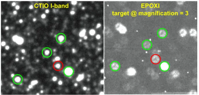
The EPOXI data consist of 4127 50 sec exposures with the “clear-6” filter. To minimize data transfer requirements, the data were taken as 128 × 128 and 256 × 256 pixel sub-frames. The first 3375 exposures used 128 × 128 sub-frames, and the last 752 images were 256 × 256 sub-frames. However, the pointing stability was such that the target occasionally drifted out of the 128 × 128 sub-frames, and it was only possible to do photometry on 2900 of these 3375 128 × 128 pixel images. An example of one of these 128 × 128 pixel images is shown on the right side of Figure 2.
The instrumental point-spread function (PSF) of the High Resolution Instrument (HRI) on the Deep Impact probe is strongly dependent on the color of the target star. In addition, the instrument is permanently defocussed, yielding a toroidal–shaped PSF. This is clearly not optimal for crowded field photometry, which typically requires a spatially varying empirical PSF model for deblending. Since we performed photometry using the Daophot/Allstar/Allframe software suite (Stetson 1994), we first required a model of the instrumental PSF that is usable by Daophot.
Instrumental PSFs have been generated by Barry (2010) for the HRI using the Drizzle algo-rithm (Fruchter & Hook 2002). In this process several hundred images of a standard star were added together to create a ten–times oversampled PSF model appropriate for that object. To ap-proximate the PSF of MOA-2009-BLG-266, with V − I = 1.82, we coadded the instrumental PSFs of GJ436 with V − I = 2.44; and XO-2 with V − I = 0.75 with weightings of 0.795 and 0.205, respectively. This composite PSF was added to an otherwise empty image in a 3 by 3 grid, with each realization downsampled to standard resolution using a center pixel shifted by ± 5 pixels in x and/or y. Daophot was then run on this image, using all 9 images to build its own internal,
double–resolution PSF model using an empirical function plus “lookup table”.
Approximately 1% of pixels in our 50s observations contain signatures of cosmic rays. We filtered these pixels using an algorithm that identifies features sharper than expected from the PSF, through pairwise comparison of neighboring pixels. These pixels were masked and objects underneath these pixels ignored when generating lightcurves. We used Daophot to detect stars in each image, and then Allstar to perform joint PSF photometry on all stars in a given image. We generated a master starlist by matching the results of the Allstar analysis using Daomatch and Daomaster. This starlist was then sent to Allframe, which simultaneously photometered all images in a self–consistent manner with regards to centroiding and deblending.
To assemble the final light curves, we first aggregated the Allframe measurements of a given star across all images. Due to the difficulty of obtaining precise flat field images in space, we cannot calibrate these images using the same methods as would be used for ground-based images. As a result, the light curves of all the stars observed by EPOXI/HRI show variations at the ∼ 1 % level on a time scale of a few hours, which is the time that it takes for the pointing to drift a distance of order the PSF FWHM. Because this is the dominant term in the EPOXI/HRI photometry errors, we bin the data at an interval of 2.4 hours, which seems to remove most, but not all, of the correlations. This gives the light curve shown in the inset in the upper right hand corner of Figure 1.
We had also hoped to get EPOXI/HRI observations after the MOA-2009-BLG-266 microlensing event had returned to its baseline brightness in March or April, 2010. Unfortunately, the EPOXI operations team was busy with preparations for the November, 2010 encounter with comet Hartley 2, so no baseline observations were possible. Therefore, we have determined the baseline brightness in the EPOXI by comparing the EPOXI images to V and I band CTIO images taken in June 2010, when the microlensing event had returned to baseline. The I band CTIO image is compared to one of the EPOXI frames in Figure 2. Because of the relatively large EPOXI/HRI PSF, we consider only stars in the EPOXI images that have only one counterpart star within a radius of 300 of the position of the EPOXI star. We also limit our consideration to stars within 0.9 mag of the V − I color of the microlensed target star. There are 4 stars that satisfy this condition and appear in more than half of the images in which the target star appears. These are the 4 stars indicated by the green circles in Figure 2. We fit the mean “clear”-filter EPOXI magnitude, CEP OXI to the instrumental CTIO magnitudes from the SoDoPHOT reductions, and this yields the following linear relationship between the average EPOXI magnitudes and CTIO magnitudes,
CEP OXI = 0.520ICT IO+ 0.480VCT IO . (1)
The fit to the magnitude of these 4 comparison stars gives χ2= 0.22 for 2 degrees of freedom if the uncertainty in the EPOXI magnitudes is assumed to be 0.004 mag. We use this formula to determine the baseline CEP OXI magnitude, and we add this to the light curve as a final measurement with an assumed uncertainty of 0.01 mag.
considered to be a procedure to calibrate the source star flux instead of the baseline brightness, which includes the brightness of any unresolved stars blended with the source. But we chose to treat the unmagnified flux estimate as an estimate of the baseline brightness as this is more conservative.
4. Source Star Properties and Einstein Radius
Planetary microlensing events typically have caustic crossing or cusp approach features that resolve the finite angular size of the source star, and MOA-2009-BLG-266 is no exception as it has clear caustic crossing features. The modeling of such features constrains the source radius crossing time, t?, and this can be quite useful because t? can be used to determine the angular Einstein radius, θE = θ?tE/t?, as long as the source star angular radius, θ? can be determined. In events such as MOA-2009-BLG-266, with a strong microlensing parallax signal, θE can be combined with the parallax measurement to yield the lens system mass. Therefore, it is important to make an accurate determination of the angular radius of the source star, θ?.
4.1. Source Star Colors and Extinction
The angular radius of the source star can be determined from its brightness and color, once the effect of interstellar extinction has been removed. We start from the CTIO V and I band magnitudes and the IRSF H band magnitude that have been determined from the best fit model. The V and I band magnitudes have been calibrated to the OGLE-III system (Udalski et al. 2008) and IRSF H band has been calibrated to 2MASS (Carpenter 2001)1. The comparison between the 2MASS and the IRSF H-band data is subject to complications due to variability and blending, because the 2MASS images, with their 2” pixels, have significantly worse angular resolution than IRSF. This means that many of the apparent 2MASS “stars” cannot be used for the calibrations because they are actually blended images of two or more stars that are resolved in the IRSF images. This makes calibration of the CTIO H band images difficult, because of the relatively small 5.5 arc min2 CTIO H field of view (FOV). Fortunately, the IRSF FOV is ∼ 60 arc min2, and it is possible to use over 400 unblended 2MASS stars for the H band calibration. These calibrations combined with the best fit light curve models yield source magnitudes of
Hs= 13.780 ± 0.030 (2)
Is= 15.856 ± 0.030 (3)
Vs= 17.677 ± 0.030 , (4)
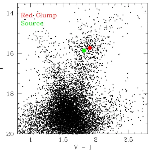
where the uncertainties are almost entirely due to the calibrations (including the uncertainty in the OGLE-III calibration. These magnitudes are indicated by the green dots in the color magnitude
1Improved calibrations are available at
diagrams shown in Figures 3 and 4. The fit uncertainties are ≤ 0.005 mag in all three passbands, and the u0 > 0 model predicts a source that is 0.005 mag brighter than the best fit u0< 0 model.
4.2. Source Star Radius
We can use the magnitudes from equations 2-4 to determine the source star angular radius, but first we must estimate the foreground extinction. We determine the source radius using the method of Bennett et al. (Bennett et al. 2010), which is a generalization to three colors of an earlier two-color method (Albrow et al. 2000). Following this procedure, we find the V IH magnitudes of the center of the red clump giant distribution to be
Hrc= 13.59 ± 0.10 (5)
Irc= 15.73 ± 0.10 (6)
Vrc= 17.64 ± 0.10 , (7)
for stars within 20 of the source star. These are indicated by the red spots in Figures 3 and 4. Assuming a distance to the source of 8.8 kpc (Rattenbury 2007), we can use these red clump magnitudes to estimate the extinction, which we find to be AH = 0.36, AI= 1.22, and AV = 2.14, following a RV = 2.77 Cardelli et al. (Cardelli et al. 1989) extinction law. These then yield de-reddened magnitudes of Hs0= 13.42, Is0 = 14.64, and Vs0= 15.54. Unlike the case for dwarf stars, the accuracy of the V − I, V − H, and I − H surface brightness-color relations (Kervella et al. 2004) is similar, but the I − H relation yields an angular radius estimate that is almost completely independent of the reddening law, if it follows the Cardelli et al. extinction law (Cardelli et al. 1989), but this may be due to the fact that the AI/AH ratio doesn’t vary much with this extinction law. In any case, all three of these relations imply that the angular radius of the source star is
θ? = 5.2 ± 0.2 µas. (8)
This and the source radius crossing time of t?= 0.326±0.007 days imply that the relative lens-source proper motion and Einstein radius are
µrel = θ?/t? = 5.86 ± 0.26 mas yr−1, (9)
and
θE= µreltE= 0.98 ± 0.04 mas, (10)
respectively.
4.3. Limb Darkening
During caustic crossings the lens effectively scans the source star with high angular resolution. As a result, the shape of the light curve reflects the underlying limb darkening of the star (Witt
1995; Bennett & Rhie 1996). Hence, in order to analyze caustic-crossing events such as MOA-2009-BLG-266, one needs to account for the limb darkening appropriately. For the previous planetary microlensing events (Bond et al. 2004; Udalski et al. 2005; Beaulieu et al. 2006; Gould et al. 2006; Gaudi et al. 2008; Bennett et al. 2008; Dong et al. 2009b; Sumi et al. 2010; Janczak et al. 2010; Miyake et al. 2011; Batista et al. 2011), limb darkening has generally been treated within the linear limb-darkening approximation. In some cases, the two-parameter square-root limb-darkening law was used (Dong et al. 2009b; Janczak et al. 2010), even though there has been no indication that the details of the limb-darkening treatment had any noticeable effect on the other model parameters for a planetary microlensing event.
In the case of MOA-2009-BLG-266, there was reason to suspect that the treatment of limb darkening could be important. This is because, as we discuss below in Section 5.1, there are two approximately degenerate microlensing parallax models that have slightly different binary lens parameters. The source crosses the caustics at a slightly different angle for the two models. This suggests that the detailed treatment of limb darkening might have some influence on the difference in χ2 between these two degenerate models. As shown by Heyrovsky (2007), using linear limb darkening may introduce photometric errors at the level of 0.01 due to the approximation itself and the choice of method used for computing the linear model coefficients. In order to avoid introducing any such inaccuracies in the analysis of the event, we directly use the limb-darkening profile from a theoretical model atmosphere of the source star, instead of its analytical approximations.
Based on the location of the source star on the color magnitude diagram, we assume a tem-perature of Teff ≈ 4750 K, surface gravity of log g = 2.5, and solar metallicity. We use a model atmosphere from Kurucz’s ATLAS9 grid (Kurucz 1996, 1993a,b)2 corresponding to these param-eters. The raw model data provide values of the specific intensity as a function of wavelength for 17 different positions on the stellar disk. In order to obtain the light-curve-specific limb-darkening profile, we integrate the specific intensity over the relevant filter passband, weighted by the filter transmission, the quantum efficiency of the CCD, and interstellar extinction (see Section 4.1). In order to compute the limb darkening at an arbitrary position on the stellar disk, we interpolate the obtained points using cubic splines with natural boundary conditions (Heyrovsky 2003, 2007). The light curve modeling code uses pre-computed tabulated intensity values for a sufficiently dense spacing of radial positions on the stellar disk.
This approach avoids a potential source of low-level systematic error without any degrees of freedom to the model. In Table 1 we compare the results of our analysis with those obtained by the usual approach, using linear limb-darkening coefficients from Claret (Claret 2000). For the parameters of the source star Claret (Claret 2000) provides coefficient values uλ = 0.7844, 0.7035, 0.6087, 0.4868, 0.4181, and 0.358 for the V , R, I, J , H, and Ks passbands, respectively. Ttabulated intensity values give a χ2 improvement over the linear approximation of ∆χ2 = 7.27 for the best-fit static models without orbital motion. So, the tabulated limb darkening tables fit
2
the data somewhat better, at least for the static lens case, but the implied planetary parameters do not change significantly.
5. Planet Characterization and Modeling 5.1. Modeling
The basic parameters for planetary events like MOA-2009-BLG-266 are straightforward to determine, as a reasonable estimate can be made from the single lens parameters (found from a fit with the planetary deviation excluded) and inspection of the light curve (Gould & Loeb 1992). The main feature of the deviation is the half-magnitude decrease in magnification centered at HJD0 = 5086.5. This indicates that a planet is perturbing the minor (saddle) image created by the stellar lens and that the star-planet separation is less than the Einstein radius. Such a light curve cannot be mimicked by non-planetary perturbations (Gaudi & Gould 1997). The basic planetary parameters can then be estimated following the arguments given in Sumi et al. (2010). In practice, this is not how the parameters were determined, however.
We model the data using standard methods (Bennett 2010; Dong et al. 2006) to extract the precise parameters and uncertainties of the light curve fit. It is convenient to describe microlensing events in terms of the Einstein ring radius, RE = p(4GML/c2)DSx(1 − x), which is the radius of ring image seen when the source and (single) lens are in perfect alignment. Here ML is the lens system mass, x = DL/DS, and DL and DS are the lens and source distances. Microlensing by a single lens, such as an isolated star, is described by three parameters: the Einstein radius crossing time, tE, and the time, t0, and distance (with respect to RE), u0, of closest alignment between the source and lens center of mass. Planetary microlensing events require three additional parameters: the planet:star mass ratio, q, the star-planet separation, s, in units of RE, and angle of the source trajectory with respect to the star-planet axis, θ. The source radius crossing time, t?, is also required because, like most planetary events, MOA-2009-BLG-266 has sharp light curve features that resolve the angular size of the source star.
The MOA and Canopus data for the event were modeled immediately upon the detection of the planetary perturbation using the method of Bennett (2010), supplemented with the addition of the hexadecapole approximation (Pejcha & Heyrovsky 2009; Gould 2008). This found the basic solution that we present here, plus a disfavored alternative s > 1 solution, which was excluded within hours when the planetary deviation data from South Africa, Israel, and Chile became available. The s < 1 solution was refined as more data came in, and the two degenerate solutions that we present here emerged when microlensing parallax was added to the modeling.
We also conducted a blind search of parameter space using the approach of Dong et al. (2006), where the binary parameters s, q, and θ are fixed at a grid of values, while the remaining parameters are allowed to vary so that the model light curve results in minimum χ2 at each grid point. A
Markov Chain Monte Carlo method was used for χ2 minimization. Then, the best-fit model is obtained by comparing the χ2 minima of the individual grid points.
5.2. Best-fit Model
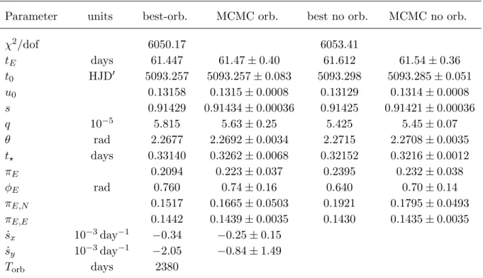
The modeling indicates that the perturbation of MOA-2009-BLG-266 is produced by the cross-ing of a clump giant source star over the planetary caustic produced by a low-mass planet. As we discuss below in Section 5.3, the orbital motion of the planet is not needed to describe the light curve. Assuming a static lens sytem, the best fit values of the planet/star mass ratio and nor-malized star-planet separation are q = 5.425 × 10⁻⁵ and s = 0.91422, respectively. The values of other lensing parameters are listed in Table 2. This table also lists the best fit parameters for fits including orbital motion. The inclusion of orbital motion improves χ2 by ∆χ2 = 3.24 for 2 fewer degrees of freedom, but it also changes the planet/star mass ratio and normalized star-planet separation to q = 5.815 × 10⁻⁵ and s = 0.91429. As discussed below in Section 5.4, the inclusion of microlensing parallax adds a parameter degeneracy that takes u0 → −u0 and θ → −θ, which corresponds to a reflection of the lens plane with respect to the geometry of the Earth’s orbit. We find that the model with u0 > 0 is favored by ∆χ2 = 13.39 for static models and ∆χ2 = 6.31 for models with orbital motion. The χ2 contribution of the individual data sets for the best models with and without orbital motion is shown in Table 1. We note that this mass ratio is the lowest of planets yet to be discovered by the microlensing method.
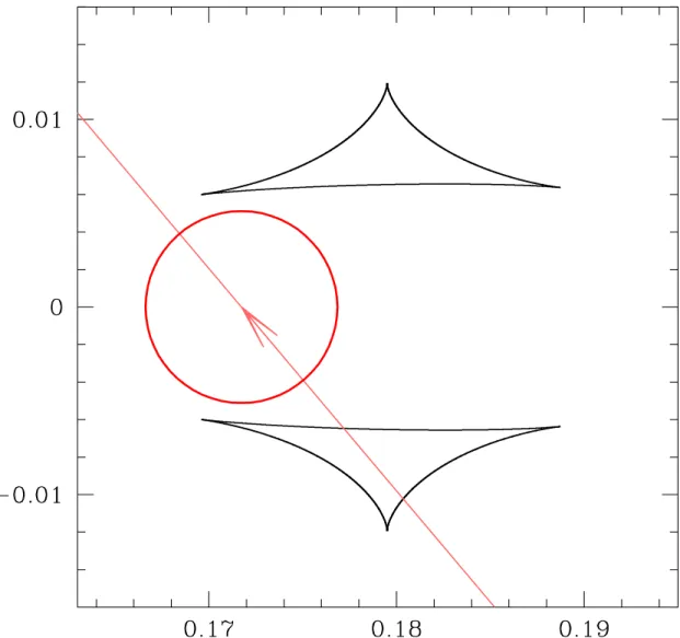
Figure 1 shows the best-fit model curve compared to the light curve data. Figure 5 compares the planetary caustic geometry to the source size and trajectory. The two triangular shaped caustics indicate a minor image caustic perturbation, which is seen when the star-planet separation is less than the Einstein radius (s < 1). The strongest feature in such a minor image caustic crossing event is the large decrease in magnification at HJD ∼ 2455086.5 when the source is between the caustics and the minor image is essentially destroyed. This feature is surrounded by two positive light curve bumps caused by the source passing over a caustic or passing in front of the cusps. There are no known non-planetary light curve perturbations that can produce such a feature in the light curve (Gaudi & Gould 1997). For MOA-2009-BLG-266, the local light curve minimum between the caustic crossings has a short duration of ∼ 3.7 hours, which is much smaller than the caustic crossing durations of > 20 hours. This is due to the fact that separation between the two triangular minor image caustics is only slightly larger than the diameter of the source star.
5.3. Orbital Motion
Like most low-mass planetary microlensing events, MOA-2009-BLG-266 can be well modeled without including any orbital motion of the planet about the host star. But, while we haven’t measured the light curve precisely enough to measure orbital motion parameters, the planetary
orbital motion does influence the precision to which the parameters can be measured from the light curve. In particular, orbital motion allows the planetary caustic to move with respect to the center of mass of the system. Thus, the planetary caustic can be either larger or smaller than the value determined from static lens models, so the mass ratio is not measured as precisely as the static models would imply. In addition, the source radius crossing time is also determined by the time it takes the source to cross the sharp light curve features of the planetary caustic, so this also depends on the orbital motion of the planet and is less precisely determined than the static models would imply.
We include orbital motion using the parameterization used for the analysis of the two-planet event OGLE-2006-BLG-109Lb,c (Bennett et al. 2010), with the x-axis defined by the vector sep-arating the star and planet at HJD = 2455086. The main orbital motion parameters are ˙sx and ˙sy, which describe the instantaneous planet velocity at the time HJD = 2455086. This parameter-ization also includes the orbital period, Torb, but this parameter has a very small effect on the χ2 value if it is in the range of physically reasonable values. So, for many of our calculations, we have left Torb fixed at a physically reasonable value. Independent calculations with a slightly different orbital motion parameterization (Skowron 2011) reached identical conclusions.
The effect of the orbital motion on the other light curve parameters can be seen in Table 2, which shows the parameters and error bars for models with and without orbital motion. The inclusion of orbital motion shifts the values of q and t? significantly, by 2.6 and 3.8 times the error bars of the static solution, respectively. Orbital motion also increases the error bar on q by a factor of 3.6 and the error bar on t? by a factor of 5.7, but the error bars on the other parameters don’t change significantly, except for the error bar on t0, which grows by a factor of 1.6. The error bars on the implied physical parameters, shown in Table 3, also don’t change very much when orbital motion is included. However, the central values of the physical parameters do change by as much as 0.4σ.
While the light curve has not been measured precisely enough to significantly constrain the orbital motion, the orbital motion can be constrained with the requirement that the planet be bound to its host star. Such a constraint requires that the mass and distance of the host star be known, but the light curve does provide this information as shown below in eqs. 13 and 14. The light curve parameters include the transverse host star-planet separation, s, and the transverse components of the planet velocity, ˙sx and ˙sy. One option is to enforce a model constraint that the orbital motion parameters are consistent with a physical circular orbit. This is equivalent to imposing a constraint on the distance to the source (Bennett et al. 2010), which we take to be DS = 8.8 ± 1.2 kpc based on the Galactic longitude of this event (Rattenbury 2007). This constraint has been employed for the best fit model shown in Table 2. But, such a constraint is inconvenient to use in our Markov Chain Monte Carlo (MCMC) calculations to determine the distribution of allowed light curve and physical parameters, as it makes it more difficult to obtain well sampled Markov Chains.
velocity not be too large to allow the planet to be gravitationally bound to the star, since the probability of lensing by a planet not bound to the lens star is ∼ 10< −8. The transverse velocity components allow us to compute lower limits on the planetary kinetic energy and gravitational binding energy (or an upper limit on the absolute value of the binding evergy). The requirement that the total energy < 0 yields an upper limit on the transverse planet velocity (Dong et al. 2009b):
˙s2x+ ˙s2y ≤ 2GML d⊥R2E
= 2GML
s(θEDL)3
, (11)
where d⊥ is the transverse star-planet separation. The R3E = (θEDL)3 factor in the denominator is needed because the planet-star separation, s, and transverse velocity components use the Einstein radius as their unit of length.
The constraint, eq. 11, has been used in all of our MCMC calculations to determine the allowed parameter distributions, and we have also added a ∆χ2= 4 penalty to potential MCMC links with a ˙s2x + ˙s2y of more than half the upper limit in eq. 11. Such parameter sets are unlikely because they require a kinetic energy higher than the average value and small values for the separation and velocity along the line of sight. Attempts to find best solutions with the eq. 11 in place of the circular orbit, source distance constraint did not yield better solutions than the one shown in Table 2.
5.4. The Parallax Effect
The microlens parallax is defined by the ratio of the Earth’s orbit to the physical Einstein radius projected on the observer plane, ˜rE, i.e.,
πE= AU
˜ rE
. (12)
Lens parallaxes are usually measured from the deviation of the light curve from those of standard (single or binary) lensing events due to the deviation of the source trajectory from a straight line caused by the orbital motion of the Earth around the Sun (Gould 1992; Alcock et al. 1995). But it is also possible to detect microlensing parallax using observations from a spacecraft in a heliocentric orbit (Refsdal 1966; Dong et al. 2007), and such satellite observations have the potential to significantly increase the number of events for which the microlensing parallax effect may be detected.
For the event MOA-2009-BLG-266, the parallax effect is firmly detected. We find that the χ2 difference between the (static) best-fit models with and without the parallax effect is ∆χ2 = 2789.3, which implies that microlensing parallax is detected at the ∼ 53σ level. The difference between the parallax and non-parallax models can be seen in Figure 1, where the best fit model is plotted as a solid black curve and the best fit non-parallax model is the grey dashed curve. Most of the parallax signal comes from the data outside of the planetary deviation. The light curve without parallax
lies below the observed data prior to the planetary perturbation and above the data after the light curve peak. Most of the signal comes from the MOA data, but good coverage of the global light curve shape from CTIO and Canopus has enabled these light curves to contribute to the parallax signal.
There are a number of degeneracies that often affect the parallax parameters of an event. For events with parallax effect, a pair of source trajectories with the impact parameter and source trajectory angle of (u0, θ) and (−u0, −θ) can yield degenerate solutions (Smith et al. 2003). Without parallax, this transformation is a trivial redefinition of parameters, but with parallax, we have the reference frame of the Earth’s orbit, which allows us to distinguish between two solutions that differ by a reflection of the lens plane. For single lens events with tE as small as ∼ 60 days, there is usually an additional degeneracy known as the jerk-parallax degeneracy (Gould 2004), but the additional light curve structure due to the planet removes some of the parameter degeneracy. As a result, the (u0, θ) ↔ (−u0, −θ) degeneracy and the jerk-parallax degeneracy are replaced by a single parameter degeneracy that makes the (u0, θ) ↔ (−u0, −θ) and changes the parallax parameter, πE. This degeneracy yields the two solutions with similar parameters, but when orbital motion of the planet is ignored, there are significant differences in the other model parameters besides u0 and θ. With no orbital motion, the u0 > 0 solution is favored by ∆χ2 = 13.39. Formally, this is quite significant as the u0< 0 solution would be disfavored by a formal probability of e−∆χ
2/2
≈ 0.0012, but we must also consider possible systematic errors that may influence the ∆χ2 value between the u0 > 0 and u0 < 0 solutions, as well as the orbital motion of the planet.
This concern about possible systematic errors was the reason for the careful limb darkening treatment described in Section 4.3. In addition, we also considered a number of different photo-metric reductions of the data sets that contribute the most to the detection of the parallax signal. These were the MOA, Canopus, and CTIO I and H band data sets. With these different photomet-ric reductions, we found that the u0 > 0 solution was always favored by a similar ∆χ2 difference, although the SoDoPHOT reduction of the CTIO I band data set and the DoPHOT reduction of the CTIO H band data set favored the u0 < 0 solution by a somewhat larger ∆χ2 difference. Table 1 indicates that the χ2 difference between the u
0 > 0 and u0 < 0 solutions is spread over a number of different data sets.
The inclusion of the orbital motion parameters discussed in Section 4.3 has a significant effect on the (u0, θ) ↔ (−u0, −θ) degeneracy. When the orbital motion parameters are included, the best fit (u0 > 0) model improves its χ2 value by ∆χ2 = 3.24, but the χ2 improvement for the u0 < 0 models is even greater, ∆χ2 = 10.34, so that the χ2 difference between the u0 < 0 and u0 > 0 solutions drops to ∆χ2 = 6.29 when the planetary orbital motion parameters are included in the models. But, an even more significant difference is that the differences between the other parameters for these degenerate models largely disappear when orbital motion is included. The added degrees of freedom provided by the orbital motion parameters appear to be larger than the light curve difference enforced by the (u0, θ) ↔ (−u0, −θ) transformation. As a result, once orbital motion is included, the (u0, θ) ↔ (−u0, −θ) degeneracy has no obvious effect on the determination
of the physical parameters of the event.
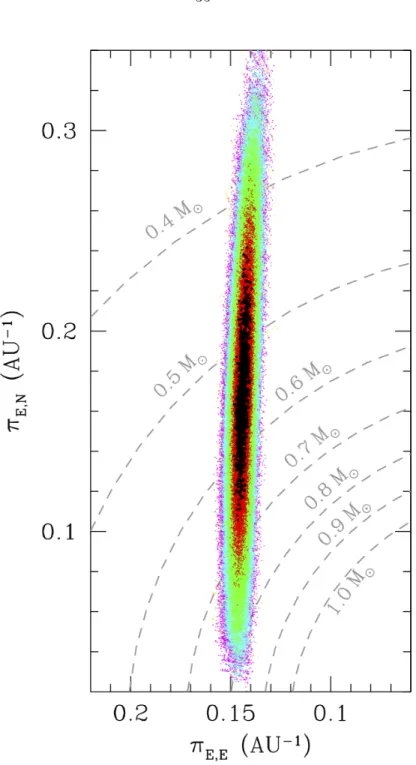
Figure 6 shows the distribution of parallax parameters, (πE,N, πE,E) or equivalently, (πE, φE) found by our MCMC simulations. This plot includes 11 separate MCMC chains with a total of 593,000 links as discussed in Section 5.5. The distributions for both solutions are highly elongated along the πE,N axis. This is due to the fact that the Earth’s acceleration is almost entirely in the east-west direction, when projected on the plane perpendicular to the line of sight to the Galactic bulge. Figure 6 also shows contours of constant πE, which are labeled by the (approximate) corresponding lens mass. The lens mass depends on the angular Einstein radius, which our MCMC calculations determine to be θE = 0.98 ± 0.04 mas. However, these mass contours in Figure 6 are only approximate because they do not include any correlations between the πE and θE values. These correlations are properly incorporated into our MCMC calculations, which yield the host star and planet masses, M? = 0.56 ± 0.09M and mp = 10.4 ± 1.7M⊕, located at a distance of DL= 3.04 ± 0.33 kpc. Assuming a random orientation of the orbit, we estimate a semi-major axis of a = 3.2+1.9−0.5AU. If we assume a standard position for the snow line, ∼ 2.7(M/M ) AU (Kennedy & Kenyon 2008), then the planet orbits at about twice the distance of the snow line, similar to the position of Jupiter in our own solar system. Thus, the planet might be considered to be a ”failed Jupiter” core as predicted by the core accretion theory (Thommes et al. 2008; Ida & Lin 2005), in which the rock-ice core only reaches ∼ 10M⊕ after the hydrogen and helium gas in the proto-planetary disk has dissipated.
In principle, any orbital parallax signal can be mimicked by so-called xallarap, i.e., orbital motion of the source about a companion (Griest & Hu 1992; Han & Gould 1997). However, this would require very special orbital parameters, basically mimicking those of the Earth (Smith et al. 2002). We search for such xallarap solutions over circular orbits, i.e., with 3 additional free parameters (orbital phase, inclination, and period). We find a χ2 improvement of 3.9 relative to the parallax solution for 3 degrees of freedom, or 3.4 with the period fixed at P = 1 year (2 degrees of freedom). These improvements have no statistical significance and are to be compared with the improvement of ∆χ2 = 2789.3 for the parallax solution relative to the no-parallax solution. Therefore, we conclude that the light curve distortions are due to parallax rather than xallarap (Poindexter et al. 2005).
Our final fit parameters are listed in Table 2. The parameters πE,N and πE,E are the North and East components of the microlensing parallax vector, πE. The uncertainty in πE,N is an order of magnitude larger than the uncertainty in πE,E because the projected acceleration of the Earth is largely in the East-West direction during this event.
5.5. Parameter Uncertainties
Uncertainties in the parameters have been determined by a set of 11 Markov Chain Monte Carlo (MCMC) runs with a total of approximately 593,000 links. Eight of these MCMC runs have
been in the vicinity of the u0 > 0 solution and the other three have been in the vicinity of the u0 < 0 local χ2minimum. Due to the χ2 difference, ∆χ2 = 6.29 between these local χ2minima, we include a weight factor to our sums over the Markov chains so that the disfavored u0 < 0 solutions are disfavored by an amount appropriate for their χ difference, e−∆χ2 = 0.043. The mean parameter values for these solutions and their uncertainties are shown in Table 2. For most parameters, these are given by the weighted averages over the 11 Markov chains, but for u0 and θ, we have included only the 8 Markov chains with u0> 0 and θ > 0. Due to the large difference in these parameters in the vicinity of the two solutions, the mean values would be values that are inconsistent with both solutions if we had used both solutions for these sums. For the remaining parameters, except ˙sx and
˙sy, the parameter distributions for the vicinities of the two local χ2 minima are nearly identical.
5.6. Physical Parameters
The source radius crossing time, t?, is an important parameter because it helps to determine the angular Einstein radius, θE = θ?tE/t?, as discussed in Section 4.2. When this is combined with the measurement of the microlensing parallax signal, we are able to determine the mass of the lens system (Gould 1992), ML= θEc2AU 4GπE = θE (8.1439 mas)πE M ≈ 0.57M . (13)
if we assume that the favored parameters of the best fit (u0 > 0) solution are correct. The lens system distance can also be determined
DL=
AU πEθE+ πS
≈ 3.2 kpc, (14)
assuming that the distance to the source, DS = 1/πS, is known. Note that these values from best fit solution are not identical to the central values from our full MCMC analysis, although they are very close.
In order to determine the physical parameters of this planetary lens system, it is important to include the effects of correlations of the parameters and the uncertainties in external measurements, such as the determination of θ?. Such a calculation is easily done with MCMC simulations. As discussed in Sections 5.4 and 5.5, we have run 11 MCMCs in the vicinity of both the degenerate u0 > 0 and u0 < 0. The distribution of the parallax parameters for these solutions is shown in Figure 6. The gray, dashed circles in this figure show the contours of constant πE, which correspond to contours of constant mass by equation 13. However, this correspondence is only approximate because θE is slightly correlated with πE.
These MCMC simulations can also be used to determine the physical parameters of the host star and its planet, which are summarized in Table 3. This is essentially a Bayesian analysis, but the only non-trivial prior that we impose is the assumption that the orbital orientation is
random, which is used to estimate the semimajor axis, a, based on the measured two-dimensional separation in the plane of the sky. If planets are much more common at very small or very large separations, then the planetary detection would imply a bias that violates this assumption. But, the available evidence indicates that planet frequency does not have a sharp dependence on the semimajor axis, so this assumption seems reasonable. Our MCMC calculations assumed a fixed distance of 8.8 kpc to the source star, due to its position on the more distant end of the Galactic bar. We have adjusted the uncertainties in Table 3 to include the 5% spread in the distance to bulge clump stars measured in this direction (Rattenbury 2007) (although the effect is quite small.) The probability distributions for the host star and planet masses and distance (M?, mp and DL) are nearly Gaussian, so they are well described simply by their mean values and dispersions. This is not the case for our estimate of the semi-major axis, a, which has a 2σ (95% confidence level) range of 2.3-12.9 AU.
We therefore conclude that the MOA-2009-BLG-266Lb the planet is a ∼ 10M⊕ planet at a separation of ∼ 3 AU. In the core accretion model of planet formation, the snow line is an important location where the density of solid material jumps by about a factor of five due to the condensation of ices (mostly water ice) (Ida & Lin 2005; Lecar 2006; Kennedy et al. 2006; Kennedy & Kenyon 2008; Thommes et al. 2008). Assuming a standard position for the snow line, ∼ 2.7(M/M ) AU, we find that the planet is located at about twice the distance of the snow line, similar to the position of Jupiter in our own solar system. It is therefore a prime candidate to be a “failed Jupiter core,” which grew by the accumulation of solid material to ∼ 10M⊕, but was unable to grow into a gas giant by the accretion of Hydrogen and Helium because the proto-planetary disk had lost its gas before the planetary core was massive enough to accrete it efficiently.
The mass measurements of the planet and host star given in Table 3 have uncertainties of about 16%, which is dominated by the uncertainty in πE,N. This uncertainty can be reduced 5-10 year hence when the source and planetary host stars have separated enough to allow their relative proper motion to be measured (Bennett et al. 2007). Since πE is parallel to the lens-source proper motion, this will reduce the uncertainty in πE to a value much closer to the 2.4% uncertainty in πE,E, which should reduce the uncertainties in the star and planet masses to < 5%. Our existing VLT/NACO observations indicate that the combined H-band flux of the source and host star is H = 13.77 ± 0.05, which is consistent with our prediction that the host star should be ∼ 75 times fainter than the source and indicate no neighbor stars that might interfere with the detection of the source-host star relative motion. So, we expect that it will be feasible to improve these mass measurements in the future.
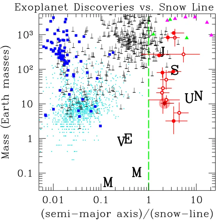
We find a host star of mass M?= 0.56±0.09M orbited by a planet of mass mp = 10.4±1.7M⊕, located at a distance of DL = 3.04 ± 0.33 kpc. Assuming a random orientation of the orbit, we estimate a semi-major axis of a = 3.2+1.9−0.5AU and an orbital period of P = 7.6+7.7−1.4yr. If we assume a standard position for the snow line, ∼ 2.7(M/M ) AU (Kennedy & Kenyon 2008), as indicated in Figure 7, then the planet orbits at about twice the distance of the snow line, similar to the position of Jupiter in our own solar system. However, the planet’s mass of ∼ 10M⊕ is close to the critical
mass predicted by core accretion theory (Thommes et al. 2008) where it has exhausted the nearby supply of solid material and begins the slow, quasistatic gas accretion phase. So, MOA-2009-BLG-266Lb fits the theoretical predictions for a large population of “failed gas giant” core (Laughlin et al. 2004) planets, which would have had their growth terminated by the loss of gas from the proto-planetary disk prior to the rapid gas accretion phase. Indeed, the distribution of planets found by microlensing, shown in Figure 7, seems to confirm this prediction, as the detection efficiency corrected planetary mass function rises steeply, as ∼ q−0.7±0.2 toward lower mass ratios (Sumi et al. 2010). However, a much sharper comparison to theory can be made with mass measurements of these planets and their host stars. Some theoretical treatments suggest a relatively sharp feature in the mass function at ∼ 10M⊕, and the low-mass end of the exoplanet mass function is likely to depend on the host star mass. MOA-2007-BLG-192Lb (Kubas et al. 2011) is the only other cold, low-mass planet with a host star mass measurement, but the planet mass is weakly constrained, due to a poorly sampled light curve.
6. Conclusions and Implications for Future Discoveries
Figure 7 shows the distribution of known exoplanets as a function of mass and separation, with the separation given in units of the snow line, which is estimated to be located at ∼ 2.7M/M AU (Ida & Lin 2004; Kennedy, private communication). (We correct the Ida & Lin formula to use scale with the stellar luminosity at the time of planet formation, ∼ 106yrs, instead of the main sequence luminosity.) The small cyan-colored dots in this plot indicate the location of the ∼ 1200 planet candidates recently announced by the Kepler mission (Borucki et al. 2011). However, these planet candidates have only radius estimates and no mass estimates, so we estimate their masses using the mass-radius formula of Traub (2011).
While there are a number of exoplanets found by microlensing with similar mass and sep-aration, MOA-2009-BLG-266Lb is the only low-mass planet from microlensing with a precisely measured mass. MOA-2007-BLG-192Lb is likely to be the lowest mass planet, at ∼ 3M⊕, found by microlensing (Bennett et al. 2008; Kubas et al. 2011), and the mass of the host star has been reasonably well determined, 0.084+0.015−0.012M due to a microlensing parallax signal and detection of the host star in high resolution AO images. However, the event was not alerted until the planetary signal was over, and as a result, the planetary light curve is poorly sampled. This results in an uncertain planetary mass ratio, so that the mass is not precisely measured.
Current and future developments in the microlensing field suggest that such mass measure-ments may become much more common in the near future. The rate of microlensing planet dis-coveries is expected to increase significantly in the near future, with the high cadence, wide-field approach of MOA-II being adopted by a number of other observing programs, such as the OGLE-IV and Wise Observatory surveys, which should begin full operations in 2011 and 2012, respectively. The most ambitious ground-based program, the Korean Microlensing Telescope Network (KMT-Net) is expected to follow a few years later (Kim et al. 2010). The observations from the EPOXI
spacecraft have made only a modest contribution to this discovery, due to the limited observing time and relatively small distance (∼ 0.1 AU) from Earth. But future observations from EPOXI or other solar system exploration spacecraft at a more typical separation of >
∼ 1 AU would be much more effective, and will be able to determine masses for most of the events that they observe. Fi-nally, follow-up images with the Hubble Space Telescope will enable mass determinations of many of the planets discovered by microlensing, after a few years of lens-source relative proper motion (Bennett et al. 2007). The results presented here illustrate that it will often be possible to precisely determine the host star and planet masses, and so measure the mass function of cold planets in the Earth-Jupiter mass range as a function of their host mass, which together with the Doppler and transit methods will provide crucial constraints on the physics of planet formation across the wide range of planet/star separations.
This discovery tends to confirm the earlier claims (Sumi et al. 2010; Gould et al. 2010) that microlensing has revealed a previously undetected population of cold, relatively low-mass planets, and the measurement of the planet and host star masses suggests that this population of planets may be related to the “failed Jupiter-cores” predicted by the core accretion theory, although there are alternative mechanisms that could form such planets (Boss 2006). Microlensing observations could provide much sharper tests of these theories if there were more discoveries with precisely measured masses.
One potentially promising avenue for such measurements is further observations with small telescopes on solar system exploration spacecraft, such as we have obtained with EPOXI. While the EPOXI observations of MOA-2009-BLG-266 have made only a modest contribution to the microlensing parallax measurement, this is a consequence of the poor light curve coverage of the EPOXI observations and the close proximity of EPOXI to Earth (∼ 0.1 AU) at the time of observa-tions. Observations from EPOXI or a similar spacecraft at a more typical (∼ 1 AU) distance, with> better light curve coverage (as might be obtained during an extended mission) would be very ef-fective at measuring lens masses. Furthermore, such a spacecraft could measure masses for planets and their host stars residing in the Galactic bulge, which is probably the case for OGLE-2005-BLG-390Lb (Beaulieu et al. 2006) and MOA-2008-BLG-310Lb (Janczak et al. 2010). These events have such short timescales that the orbital motion of the Earth is very unlikely to allow the measurement of the microlensing parallax, but in most cases, a telescope in a heliocentric orbit at ∼ 1 AU will> be able to measure the microlensing parallax effect and determine the planet and host star masses. Of course, the study of low-mass planets beyond the snow line would benefit greatly from an increased discovery rate over the current rate of ∼ 4 per year. The original strategy for finding planets by microlensing (Mao & Paczy´nski 1991; Gould & Loeb 1992) was to have one wide field-of-view telescope identify microlensing events that are then observed by a global network of narrow field-of-view follow-up telescopes. This strategy was developed in 1992 and was expected to find Jupiter-mass planets in Jupiter-like orbits. It has proved not to be very efficient for lower mass planets, although some important discoveries have been made (Beaulieu et al. 2006).