ABSTRACT: The point-like quasi-steady aerodynamic loading in a turbulent flow is formally expressed as a function of the squared relative velocity between the fluid and the investigated structure. The three major terms governing the low-order statistics of the response are known to be related to the average loading, the linear turbulent loading and the aerodynamic damping. The three other terms in the loading, namely the quadratic turbulence term, the parametric velocity feedback term and the squared velocity term, may significantly affect the higher order statistical cumulants of the response. These latter two sources of fluid-structure interaction are usually disregarded, by lack of efficient simulation tools, except a Monte Carlo simulation of the nonlinear equation. In this paper, we provide a formal analysis of the complete nonlinear model, including thus all six terms, but mainly focusing on the importance of the two nonlinear coupling terms of the loading. Closed form solutions of the response are derived for a second-order Volterra model of this problem, under the assumption of different timescales in the loading and in the structural behavior. Two major outcomes of the analysis are, on the one hand, that the squared structural velocity term has no influence on the cumulants of the response up to order 4 and, on the other hand, that the parametric velocity feedback acts as a reduction of the non Gaussianity of the response.
KEY WORDS: Volterra model; Multiple Timescale Spectral Analysis; squared velocity feedback; parametric; turbulence.
1 INTRODUCTION
The response of civil engineering structures to the wind turbulence is a multiple timescale process. Indeed, in a linear context, the structural response to very low frequency turbulence excitation may be approached by a sum of two components, a background component associated with the slow dynamics of the excitation and a fast resonant component associated with the structural timescale [1].
The stochastic structural analysis of a linear structure subject to a stationary excitation, such as the wind turbulence, is usually performed with a spectral approach. While offering a clear understanding of the structural behavior and the dispatching of energy in the different timescales, this approach also sidesteps the heavy generation of the wind velocity or pressure time histories. The stochastic approach is a useful tool to determine the Gaussian, but also non-Gaussian, response of a linear system. One drawback perhaps is that the evaluation of high-order statistics requires a multi-dimensional integration of spectral densities in spaces whose dimension increases with the order of the cumulants of the response under investigation. The application of the method in the context of non-Gaussian responses thus turns out to be challenging, from a computational viewpoint. This drawback is partly circumvented by considering the existence of the different timescales in the response. Doing so, the multiplicity of the integrals to be computed is decreased by one, which substantially speeds up the computation [2].
In this paper, the concept described above is extended to the study of a linear oscillator whose excitation is defined as a quadratic function of the wind-structure relative velocity. The analysis still relies on a spectral approach and the structural system is modeled as a Volterra system [e.g. 3].
Developments are limited to the second-order Volterra operator which is shown to be accurate enough for the statistics up to order 4. The efficiency of the method is discussed with the determination of the first four cumulants of the response. The quality of the result is assessed in terms of accuracy with respect to a reference solution obtained through Monte Carlo simulation.
2 GOVERNING EQUATIONS
Under the quasi-steady assumption, the response of a point-like single degree-of-freedom structure subject to a 1-dimensional wind turbulence is governed by the nonlinear second order differential equation
21 2 d
mx cx kx C A U u x (1) where x(t) is the structural displacement, m, c and k are mass, viscosity and stiffness, respectively, U is the mean wind velocity and u(t) a Gaussian zero-mean random process representing the wind velocity fluctuation; , A and Cd are,
respectively, the air density, the area of the structure exposed to the wind and the aerodynamic drag coefficient. The overhead dot denotes differentiation with respect to time t. The nonlinearity of this equation results from the squared structural velocity x t and the parametric excitation 2( )
2 ( ) ( )x t u t
terms obtained in the right-hand side after expansion.
The zero-mean Gaussian turbulence process u(t) is fully described by its power spectral density Su(). Following
Kolmogorov’s energy cascade, typical models for the turbulence decrease as -5/3 in the high-frequency range. This non Markovian behavior makes any stochastic method based
Efficient estimation of the high-order response statistics of a wind-excited oscillator
with nonlinear velocity feedback
Vincent Denoël1, Luigi Carassale2
1
Structural Engineering Division, University of Liège, Chemin des Chevreuils, B52/3, 4000 Liège, Belgium
2Dept. of Civil Chemical and Environmental Engineering, University of Genova, Via Montallegro, 1, 16145 Genova, Italy
on the FPK equation and moment equation rather intricate since a proper approximation with a Markovian process has to be formulated. This argument drove the solution procedure of the considered problem toward spectral methods. It is thus possible to handle realistic power spectral densities of the wind turbulence such as
2 5/3 0.546 ; 1 1.64 u u L L U S U L U (2)
in which L represents the integral length scale and u the
standard deviation of the turbulence velocity.
This problem might be formulated in a dimensionless manner leading to the governing equation
1 1 2 2 2 2 2 2 2 2 s a u u a u a u x x x u I u I ux I x I (3)where the following dimensionless quantities are used
0 2 0 0 , , , , , 2 2 u d u d s a o k u k x x u t t t m AC I U AC U c U m m L (4)
and where a prime denotes differentiation with respect to the nondimensional time t . The power spectral density Su( ; ) of the dimensionless turbulence velocity u is a function of the dimensionless frequency and of the small parameter , which is the ratio of the characteristic turbulence frequency
U/L and the structural natural frequency 0. The two
coefficients s and a represent the structural and aerodynamic
damping coefficients.
This formulation indicates that the solution of the problem at hand may evolve in different regimes, depending on the relative smallness of s, a and . These three numbers are
typically in the range [10-3; 10-1]. A fourth small parameter of the problem is the turbulence intensity Iu, usually in the range
[10%; 30%], which scales the quadratic turbulence term and the nonlinear feedback terms on the right hand side of Eq. (3). The dimensionless version of the governing equation readily shows that the quadratic velocity term x² is one order of magnitude smaller than its left neighbor ux, the parametric excitation term, which presumably indicates that the former one would yield negligible contribution to the response. This is to be proved with a more formal derivation. Although the dimensionless version of the governing equation is definitely more convenient to identify the leading physics and its limiting cases, the paper is mainly developed with physical quantities, so as to provide a simpler understanding.
3 SECOND ORDER VOLTERRA MODEL
3.1 The Volterra Frequency Response Functions
Inspired by former works [4], it is chosen to model the response of this nonlinear problem with a second order Volterra model. This choice is validated in Section 5, with the typical orders of magnitude of the parameters encountered in wind engineering applications.
In this framework, the response x(t) is expressed as
1 2
( ) o
x t x x t x t (5) where x1(t), respectively x2(t), is defined as the first (resp.
second) order convolution of the zero-mean Gaussian input
u(t) with the Volterra kernel h1(t), respectively h2(t). In a
stationary setting, this definition is advantageously translated into the frequency domain with the symmetrical Volterra frequency response functions H1() and H2().
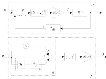
These functions need to be established for the specific nonlinearity of the problem under consideration. This may be achieved with the harmonic probing technique [5] or with the systematic procedure presented in [4]. The same procedure as that developed in the later one is being followed next. In the block diagrams of Figure 1, the differential operator [x]=
m
x
c
x
kx
actually corresponds to the forcing term (including the feedback) such that f= [x], and the operator represents the assembled I/O relationship, such that x= [u]. It results f= [ [u]] or again, by definition of the operatorf= [u].
Applying the construction rules in [4], the frequency response functions of [.]= [ [.]] are thus expressed in terms of those of and as
0 0 1 1 2 1 2 2 1 2 1 2 0 , , , , F H D F H D F H D (6) where
2 D m j c k.This sort of feedback is particularly well suited to the unwrapping of the system, in which case the forcing term f may also be expressed as in the second block diagram, as the amplification of the square of the output of operator , in which case
2 0 0 1 0 1 2 1 2 1 1 1 2 0 2 1 2 , , 2 , , . 2 d d d d C A F B F C AB B C A F B B C AB B (7)Operator is nothing but the addition of three terms, so that
0 1 1 1 2 1 2 2 1 2 1 2 2 1 2 , 1 1 , , , , , B U B A j H B A j H (8)on account that A0=0 as a result of the differential nature of
operator . Plugging these expressions backwards until Equation (6), and solving for H0, H1 and H2 yields
2 0 1 1 1 1 2 1 2 2 1 2 1 2 1 2 , , 2 1 1 , 2 d d d d d C A C AU H U H k D j C AU j H j H C A H D j C AU (9)Figure 1. Block diagram of the considered problem. These frequency response functions are sketched in Figures 2 and 3. The first one corresponds to the classical frequency response function of a linear oscillator, with additional aerodynamic damping. The second represents the interaction between the different harmonics in the response, especially the filtering of pairs of harmonics (1, 2) that fall out of the
band 1 2 o.
Figure 2. First-order frequency response function.
3.2 Cumulants of the Stationary Response
In a second-order Volterra model, the total response is expressed as the sum in Eq. (5) involving the 0th-order constant term x0, together with the fluctuating terms x1(t) and
x2(t). When the input u(t) is a stationary random process, the
statistical properties of the total response x(t) may be expressed in terms of its cumulants, which in turn can be written as functions of the cumulants of x1(t) and x2(t). Using
some classical developments in the theory of probability [6] under the hypothesis that u(t) is Gaussian distributed, we obtain
2 2 1 2 2 3 3 1 1 2 3 2 4 4 1 1 2 2 4 2 3 , , 6 , , , x x x x x x x x x x x x x x (10)where k[ ] represents (when used with a single argument) the kth-order cumulant of the argument and k[ ,..., ] represents the kth-order cross-cumulant associated with the product of the arguments.
An analysis of the orders of magnitude of the two terms that compose each cumulant of the response reveals that the second terms in the expressions given in (10) are negligible in front of the first terms, at least for the small realistic values of the aerodynamic damping a encountered in typical wind
engineering applications. The formal demonstration of this statement goes beyond the scope of this paper but is available in [7] together with a deeper investigation of this problem.
Intuitively however, the second order response x2(t) is one
or several orders of magnitude smaller than the first order response x1(t). The ratio of these two actually scales with the
aerodynamic damping a. As a consequence, in (10), the
cross-cumulant, involving more factors in x1(t) than the
unilateral cumulants of x2(t) are expected to be leading.
3.3 The Associated Linear Equations
Alternatively to the frequency domain approach, it is interesting to regard a Volterra model with its associated linear equations, which are linear ordinary differential equations describing the dynamics of each term in the expansion (5). For some sorts of nonlinearities, such as the polynomial nonlinearity of the problem at hand, the nth-order response xn(t) might be expressed, with the associated linear
equations, as a function of the forcing term and of lower order responses [8]. For the considered problem, these equations read:
0 1 1 1 2 2 2 2 2 2 1 1 1 2 2 1 2 2 2 2 u s a s a u u a u a x I x x x u x x x I u I ux I x (11)These equations confirm that x2(t) is well one or two orders
of magnitude smaller than x1(t). These equations will be used
later in a Monte Carlo simulation, in order to validate the truncation of the Volterra series to the second order.
3.4 Power Spectral Density and Higher Order Spectra of the Response
The power spectral density of the total response x(t) of a second-order Volterra model reads
2 1 2 2 1 1 1 1 1 2 , d x u u u S H S H S S
(12)where Su() is the power spectral density of the turbulence,
while H1 and H2 represent the Volterra frequency response
functions, as given in (9).
The integration of the power spectral density Sx() provides
the second cumulant of the total response
2 x Sx d
(13)Substitution of (12) into (13) indicates that the cumulant of the response is composed of two terms, as hinted by (10) anyway. The first one, involving |H1()|, is responsible for the
linear counterpart of the response 2[x1], while the second
term, involving the second-order frequency response function |H2(1,2)| provides the second contribution 2[x2] to the total
cumulant, after integration along the real axis. Following the former observation that the second terms in (10) are negligible, the second term in the power spectral density of the total response is dropped.
It finally turns out that the second order response is that of a linear system whose total damping is represented by the sum of the structural and aerodynamic dampings. In this context, there exists a classical way to bypass the numerical integration of Sx() in (13). It is based on the background/resonant
decomposition of the response, a two-timescale approximation of the response usually attributed to the pioneering works of A. Davenport [1]. In this method, the variance of the response is simply expressed as the sum of a background and a resonant component as
2 x 2 x1 1 r 2,B (14) where
2 2, ; 2 2 u o d u o B s a u S C AU r k (15)are readily interpreted as the background response and the resonant-to-background ratio.
One major advantage of this two-timescale method is that it sidesteps any integration and offers an approximate solution of the problem at no computational costs. Extension of this method to higher-order statistics was the key motivation for the consideration of this problem as a Volterra model.
Similarly to the power spectral density, the bispectrum of the total response x(t) is composed of two terms, among which only the first one is retained in the analysis, as it is responsible for the contribution 33[x1, x1, x2] to the third cumulant. The
bispectrum of the response is thus approximated as
1 2 1 1 2 1 1 2 1 2 1 1 2 1 1 1 2 1 2 2 1 2 2 1 2 2 1 1 1 1 2 1 2 1 2 , 2 , 2 , 2 , x u u u u u u B H H H S S H H H S S H H H S S (16)and the third cumulant of the response is approximated by
3 x 3 3 x x x1, ,1 2 Bx 1, 2 d 1 2
(17)Similarly again, the trispectrum of the total response x(t) is composed of two terms, among which only the first one is considered. In this simplified version, it reads
3 1 2 3 1 , , 1,2,3 1 2 2 1 2 2 , , 4 , , , , x u u u u u T H S H H H S S H H H S S
(18)where the summation is performed on all six possible permutations of the indexes , , = 1, 2, 3. The fourth cumulant of the response is thus approximated by
4 4 1 1 2 2 1 2 3 1 2 3 6 , , , , , d d d x x x x x x T
(19)The purpose of the rest of the paper is to provide simple expressions for the integrals in (17) and (19).
4 MULTIPLE SCALE SPECTRAL ANALYSIS & ANALYSIS OF THE MODEL
4.1 Cumulants of the response
The multiple timescale spectral analysis is a recent technique that allows decreasing by one (at least) the order of integration in the determination of the cumulants of the response. It hinges on the timescales separation between the loading and the structure and is able to deal with linear/nonlinear structures, stationary/evolutionary problems, SDOF/MDOF problems, and is fundamentally not limited regarding the statistical order [2]. The method is elaborated in the frequency domain and is not contingent upon the markovianity of the loading process; it thus deals with any complex analytical expression of the power spectral density of the loading –such as those that characterize the wind turbulence– without any artifact. The technique actually generalizes the background/resonant decomposition of the variance [1] and the background/biresonant decomposition of the third cumulant [9] of the response of a single degree-of-freedom linear system subject to slow stochastic loading.
Application of the general method requires the identification, in the response spectra, of the different components to the response. Among them the background component is easily identified. Its trivial subtraction from the initial response spectra leaves us with resonant and mixed background/resonant terms. Examples of applications in [2] give some hints on how to determine and approximate these components.
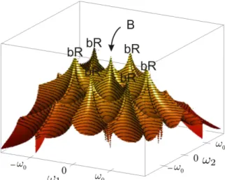
Figure 4. Sketch of the bispectrum of the response, (16). At third order, the bispectrum of the response is expressed by (16) at leading order. This function is represented in Figure
4 which illustrates the background component as a central peak of the frequency space as well as six peaks, coined as
biresonance peaks as they correspond to resonance in two
factors out of three in the each term of Bx(1,2). These peaks
are located at (1,2)= (±o), (0,±o) and (±oo).
The background contribution to the integral in (17) is obtained by replacing the frequency response functions H1
and H2 by their local behavior in (16), i.e. H1()=CdAU/k
and H2(1,2)=CdA/2k, which yields
3 3, 3 d u B u C AU I k (20)
Applying the procedure recommended in the multiple timescale spectral analysis, the additional contribution of the biresonance peaks is obtained after introduction of stretched coordinates whose purpose is to formally focus on one of these peaks, namely
1 o 1 s a 1 ; 2 o s a 2,
(20) then to approximate locally the integrand, especially the power spectral density of the wind turbulence velocity to finally obtain 3, 3, 1 2 s a R B s a r (21)
with r the second-order resonant-to-background ratio introduced in (15) and
2 2 1 2 2 2 2 4 ; ; d 4 u o u o u o S S
(22)and where the shorter notation = s + a is used. The total
cumulant of the response is finally written as the sum of the background and biresonant components, 3,B + 3,R.
The appreciable outcome of the method is that the order of integration to determine the third cumulant of the response has dropped from 2, in (17), to 1 in (22), as a result of the timescales separation.
A graphical representation of the trispectrum of the response (18) is a bit more involved as it concerns a function of three parameters. However the generic procedure developed at the third order may be replicated. It reveals the existence of four types of peaks, namely (i) a background peak located at the origin, as usual, (ii) four A-type mixed
background-resonant peaks located in
(1,2,3)=±() and (1,2,3)=(,±), (iii) two
B-type mixed background-resonant peaks located at
(1,2,3)=±(0,and (iv) four (purely) resonant
peaks located at (1,2,3)=±(and
(1,2,3)=±(.
The natures of these peaks are different because they each maximize different factors in the expression of the trispectrum. To keep it simple, the background peak corresponds to the only possible value of (1, 2, 3) that
maximizes the factors in Su, while the four resonant peaks
correspond to the four possible combinations of (1, 2, 3)
A- and B-type peaks maximize one (or two) factors in H1 or H2 and two (resp. one) factors in Su.
Resorting again to the basic principles of the multiple timescale spectral analysis [2], one may identify a background contribution 4 2 4, 12 d u B u C AU I k (23)
with the same local approximation for H1 and H2 and the
various (eventually mixed) resonant contributions. Each of these latter ones are obtained with an adequate rescaling of the problem, that aims at sequentially focusing on each kind of peak (and sort of bring to problem to the right timescale), providing a local approximation of the response at that timescale and finally return to the physical frequency space with a much simpler expression. After some involved but noteworthy calculus, the resulting expressions for those contributions read 4, 4, 1 4, 4, 2 3 2 4, 4, 1 2 2 I II s a BR B s a a BR B s a a s R B s a r r r (24)
with 2(Su( ); o; ) and 3(Su( ); o; ) are defined as
2 2 1 2 2 2 2 2 2 2 1 2 1 2 4 d d 4 u u o u u o S S
(25)
1 2 3 2 2 2 2 4 4 2 2 1 2 1 2 1 2 2 2 2 2 2 2 2 2 2 1 2 1 2 2 32 8 d d 4 4 4 u u u u o o o o o S S
(26)Similarly to the third order, we observe that the fourth cumulant of the response is simply expressed as the sum of four components, 4,B + 4,BRI + 4,BRII + 4,R, instead of the more complex triple-fold integral in (19).
In our formulation, integrals are hidden in the coefficients 1, 2 and 3, but the dimensionality of the integrals is
limited to 2, or even to 1 when mixed background-resonant components are dropped (which unfortunately degrades the quality of the result, see [10]).
4.2 Skewness and Excess Coefficients
The skewness and excess coefficients of the response are readily obtained from the corresponding cumulant. With the multiple timescale approximation, they read
1 3 3/ 2 2 1 3 1 s a s a u r I r (27)
2 1 2 3 1 2 2 2 2 1 12 1 a s s a a s a s a s a e u r r I r (28)What this model offers is a simple and attractive procedure for the computation of the skewness and excess coefficients of the nonlinear response of the considered problem. These coefficients are simply expressed as a function of the resonant-to-background ratio denoted by r, the damping coefficients, structural and aerodynamic, as well as the coefficients 1, 2 and 3 which holds the remaining
computational issues.
Interestingly enough, these latter coefficients have closed-form asymptotic expressions, for large and small values of the total damping coefficient. The relative smallness has to be assessed by comparison with the ratio of the characteristic frequency of the wind velocity turbulence and that natural frequency of the structure, introduced in (2). For instance, one may observe that all three factors tend to 1 when ≫. This makes the estimation of the skewness and excess coefficients of the response promptly accessible.
The amplitude of the nonlinearity scales with the magnitude of the aerodynamic damping, see (2). For small values of that parameter, the response is still non-Gaussian as a result of the square transformation of the wind velocity turbulence u². In the limit case, the structural behavior is linear and the current formulation degenerates into existing approximation based on the multiple timescale spectral analysis too [9]. What mainly matters here is that the non-Gaussianity of the response (measured by the magnitude of the skewness and excess coefficients) decreases as some nonlinear feedback is injected into the structure. This is readily observed by substituting a
by 0 in (27) and (28); the coefficients of 1, 2 and 3 are
systematically decreased. This validates the following statement. The differentiation in the feedback loop acts as a highpass filter of the structural response. It is well known that the non-Gaussianity of the response mainly results from the low-frequency content while the resonant component of the response is simply Gaussian. Consequently the correction to the open-loop system is more or less Gaussian and this tends to diminish the non-Gaussianity of the loading. The model described in this paper is a simple tool to quantify this return to the Gaussian distribution.
The few details that were communicated in this paper are not really sufficient to understand that the local approximations of the kernel, that allowed the derivation of the low-dimensional integral solutions, are actually not affected by the presence of the square velocity feedback. In other words, the squared structural velocity
x
2(
t
)
term is definitely negligible in front of the parametric excitation2 ( ) ( )x t u t
term, no matter the values and relative smallness of the parameters of this problem. The only limitation on this observation is that the timescales remain well separated.
At last but not least, another interesting case is that of a small dynamic amplification, in the second-order sense, i.e.
r≪. In that case, both the mixed and resonant contributions vanish and the skewness and excess coefficients of the response match those of the quadratic transformation of the Gaussian wind velocity turbulence, i.e. 3=3Iu and e=12Iu².
5 NUMERICAL APPLICATION
A Monte Carlo simulation of the three associated linear equations (11), solved sequentially, provides realizations of the total response x(t) as a sum of the deterministic 0th-order response x0 and of the realizations of the stochastic processes
x1(t) and x2(t). With the help of an online averaging method,
the raw moments of x(t), x1(t), x2(t) are readily obtained. They
are finally translated into cumulants, as they offer a more convenient understanding. They are represented in Figure 4, which shows in dashed lines the standard deviation, the skewness and excess coefficients of the total response x(t).
In a similar manner, the cumulants of the original system are obtained with a statistical processing of the Monte Carlo response of the full nonlinear equation (3), in its dimensionless version. They are reported in Figure 4 with solid lines.
They virtually correspond for the standard deviation and the skewness coefficient, while the agreement is respectable for the excess coefficient. Actually, concerning this latter one, a third-order Volterra model globally would have offered an accuracy similar to that we have for the second and third cumulants with the second-order model, but this option was not retained in this study. Notice secondarily that the inaccuracy of the second-order model grows, as expected, with the aerodynamic damping a, i.e. with the magnitude of
the nonlinearity.
The results obtained with the analytical model are represented by dots and labeled “Analytical model”. Despite the obvious simplification in the computation of the third- and fourth-order cumulants, there is a remarkable agreement between the exact result of the complete problem, including all sorts of nonlinearity, and this much simpler model.
The discrepancy on the skewness coefficient 3 features the
same order of magnitude as that on the standard deviation, which is represented in the upper plot. As the traditional background/resonant decomposition is now part of every wind engineer’s toolbox, we should agree that the slight discrepancy on the estimation of the skewness coefficient is thus also acceptable.
The discrepancy on the excess coefficient is a bit larger, especially for small structural damping coefficient. The discrepancy is similar, in magnitude, to the error in the results of the Volterra model, as compared to the full nonlinear problem. Thus, should one consider the second order Volterra model as reliable, the result of the analytical model, which is obtained at a fraction of the cost of the results of alternative options, should also be accepted.
As far as the computational efficiency is concerned, it should be emphasized that the analytical solution is extremely convenient when the two timescales involved in the problem are very different from each other, i.e. is small. In this case, indeed, the Monte Carlo simulation requires the integration of very long time series using a small time step. The computation of the results shown in Figure 4 (80 points of the parameters space, 4 values of s and 20 for a) required about one minute
for the analytical solution and about 500 hours CPU time for the Monte Carlo simulation (mostly used for the solution of the full nonlinear system).
Figure 4. The cumulants of the response of the nonlinear system (1), solid lines, agree rather well with the cumulants of
the response of the second-order Volterra model, dashed lines (obtained from the solution of the associated linear equations).
Dots represent the approximation of the cumulants obtained with the analytical solution developed in Section 4. The standard deviation is scaled by a characteristic response.
6 CONCLUSIONS
There are two main contributions in this paper. The first one concerns the derivation of the very general solution, expressed as accurate approximations though, of the stochastic response of a second-order Volterra model. Equations presented in this paper are rather general and might be applied in other fields or problems, as long as the timescales separation hypothesis holds.
The second contribution concerns the application the a classical problem of wind engineering, namely the influence of the nonlinear quadratic velocity and parametric loading terms arising in a quasi-steady aerodynamic loading. Although not given with full details, the derivation demonstrates that the parametric loading term is mainly responsible for the non-Gaussianity of the response, while the squared structural velocity term has very few influence. As an interesting outcome too, it is demonstrated that the nonlinear quadratic velocity feedback systematically reduces the skewness and excess coefficients of the loading.
REFERENCES
[1] Davenport , A. G. (1961). "The application of statistical concepts to the wind loading of structures." Proceedings of the Institute of Civil Engineers 19: 449-472.
[2] Denoël, V. (2014), “Multiple Timescale Spectral Analysis”. Submitted to Probabilistic Engineering Mechanics.
[3] Schetzen, M., The Volterra and Weiner theories of nonlinear systems, John Wiley & Sons, Inc., New York, 1980.
[4] Carassale, L. and A. Kareem (2010). "Modeling nonlinear systems by Volterra Series." Journal of Engineering Mechanics ASCE 136: 801-818.
[5] Bedrosian, E. and S. O. Rice (1971). "Output properties of Volterra systems (nonlinear systems with memory) driven by harmonic and Gaussian inputs." Proceedings of the IEEE 59(12): 1688-1707. [6] Papoulis, A. (1965). Probability, Random Variables, and Stochastic
Processes. New York, McGraw Hill.
[7] Denoël, V. and Carassale L. (2014). “Response of an oscillator to a random quadratic velocity-feedback loading”. Under preparation. [8] Feijoo, J. A. V., et al. (2005). "Associated linear equations for volterra
operators." Mechanical Systems And Signal Processing 19(1): 57-69. [9] Denoël, V. (2011). "On the background and biresonant components of
the random response of single degree-of-freedom systems under non-Gaussian random loading." Engineering Structures 33(8): 2271-2283. [10] Denoël, V. (2012). Extension of the Background/biResonant
decomposition to the estimation of the kurtosis coefficient of the response. Uncertainty in Structural Dynamics 2012. Leuven, Belgium: 11 p.