HAL Id: tel-01820663
https://tel.archives-ouvertes.fr/tel-01820663
Submitted on 22 Jun 2018HAL is a multi-disciplinary open access
archive for the deposit and dissemination of sci-entific research documents, whether they are pub-lished or not. The documents may come from teaching and research institutions in France or abroad, or from public or private research centers.
L’archive ouverte pluridisciplinaire HAL, est destinée au dépôt et à la diffusion de documents scientifiques de niveau recherche, publiés ou non, émanant des établissements d’enseignement et de recherche français ou étrangers, des laboratoires publics ou privés.
networks
Francesca Mastrogiuseppe
To cite this version:
Francesca Mastrogiuseppe. From dynamics to computations in recurrent neural networks. Physics [physics]. Université Paris sciences et lettres, 2017. English. �NNT : 2017PSLEE048�. �tel-01820663�
THÈSE DE DOCTORAT
de l’Université de recherche Paris Sciences et Lettres
PSL Research University
Préparée à l’École Normale Supérieure
From dynamics to computations in recurrent neural networks
COMPOSITION DU JURY :
M. LATHAM Peter
Gatsby Computational Neuroscience Unit - UCL London, Rapporteur
Mme. TCHUMATCHENKO Tatjana
Max Planck Institute for Brain Research Frankfurt, Rapporteur
M. HENNEQUIN Guillaume
University of Cambridge, Membre du jury M. PAKDAMAN Khashayar
Université Paris Diderot, Directeur du jury
M. NADAL Jean-Pierre
École Normale Supérieure, Invité
Soutenue par
F
RANCESCAMASTROGIUSEPPE
le 04 décembre 2017
Ecole doctorale n°
564
ÉCOLE DOCTORALE PHYSIQUE EN ÎLE-DE-FRANCE
Spécialité: Physique
Dirigée par Vincent HAKIM
et Srdjan OSTOJIC
Preface
This thesis collects the work that I have been carrying out in the last three years as Ph.D. student at ENS. During my time here, I collected some results, some failures, and good and bad feedbacks. I have been learning and growing up, and this has been possible thanks to the help of several people that I do need to acknowledge.
To begin with, I would like to deeply thank my two directeurs de thèse, who gave me the chance to start this journey. Here I had all the best opportunities to learn: that made me feel an extremely fortunate student. More than anything, I would like to thank Srdjan for having been a generous advisor, a caring supervisor, and – above all – such a nice person to work with. I am extremely thankful to all the members of the jury, who agreed dedicating their time in reading and listening about this research. I would like to thank all the teachers that I met during the summer schools in Woods Hole and Lisbon as well.
I cannot conclude without mentioning all the sweet people that worked and work at the GNT, who contribute to make our office such a friendly and cosy place where to study (and watch movies, and do yoga…). Here I felt at home like a piece of butter on a tradi. I would like to thank all the zie, and in particular Agnese, for having proofread all my motivational letters and having patiently supported me and my Ph.D. on a daily basis. To conclude, huge thanks to my family and to Riccardo, who remind me that I’m troppo forte every time I seem to forget.
Contents
1 Introduction 1
1.1 Irregular firing in cortical networks . . . 1
1.1.1 Irregular inputs, irregular outputs . . . 3
1.1.2 Point-process and firing rate variability . . . 5
1.2 Chaotic regimes in networks of firing rate units . . . 6
1.3 Outline of the work . . . 9
I Intrinsically-generated fluctuations in random networks of excitatory-inhibitory units 13 2 Dynamical Mean Field description of excitatory-inhibitory networks 17 2.1 Transition to chaos in recurrent random networks . . . 18
2.1.1 Linear stability analysis . . . 18
2.1.2 The Dynamical Mean Field theory . . . 20
2.2 Fast dynamics: discrete time evolution . . . 23
2.3 Transition to chaos in excitatory-inhibitory neural networks . . . 25
2.3.1 The model . . . 26
2.3.2 Linear stability analysis . . . 26
2.3.3 Deriving DMF equations . . . 28
3 Two regimes of fluctuating activity 33 3.1 Dynamical Mean Field solutions . . . 33
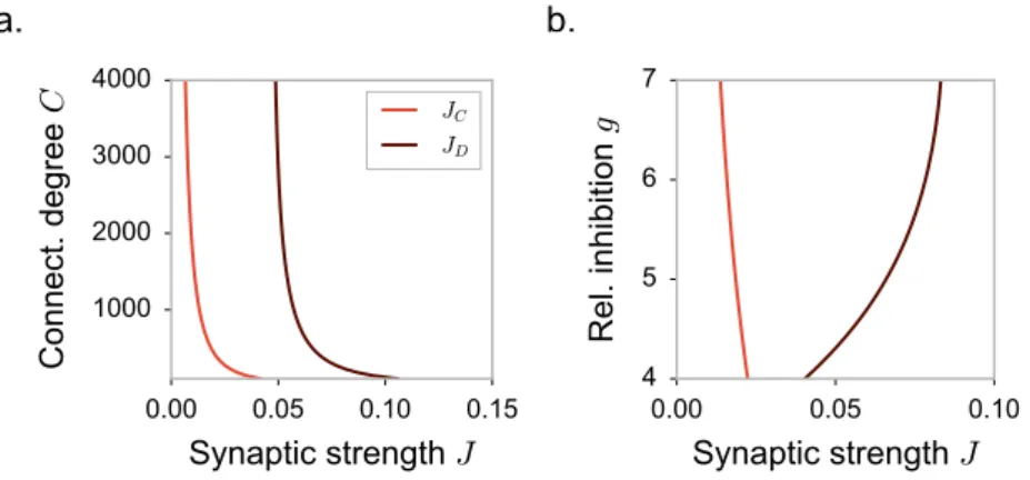
3.2 Intermediate and strong coupling chaotic regimes . . . 35
3.2.1 Computing JD . . . 36
3.2.2 Purely inhibitory networks . . . 38
3.3 Extensions to more general classes of networks . . . 39
3.3.1 The effect of noise . . . 40
3.3.2 Connectivity with stochastic in-degree . . . 42
3.3.3 General excitatory-inhibitory networks . . . 44
3.4 Relation to previous works . . . 45
4 Rate fluctuations in spiking networks 49 4.1 Rate networks with a LIF transfer function . . . 50
4.2 Spiking networks of leaky integrate-and-fire neurons: numerical results . . . . 52
4.3.1 Mean field theories and rate-based descriptions of integrate-and-fire
networks . . . 55
II Random networks as reservoirs 59 5 Computing with recurrent networks: an overview 61 5.1 Designing structured recurrent networks . . . 61
5.2 Training structured recurrent networks . . . 63
5.2.1 Reservoir computing . . . 63
5.2.2 Closing the loop . . . 65
5.2.3 Understanding trained networks . . . 66
6 Analysis of a linear trained network 71 6.1 From feedback architectures to auto-encoders and viceversa . . . 71
6.1.1 Exact solution . . . 72
6.1.2 The effective dynamics . . . 74
6.1.3 Multiple frequencies . . . 77
6.2 A mean field analysis . . . 77
6.2.1 Results . . . 80
6.3 A comparison with trained networks . . . 80
6.3.1 Training auto-encoders . . . 82
6.3.2 Training feedback architectures . . . 82
6.3.3 Discussion . . . 84
6.4 Towards non-linear networks . . . 85
6.4.1 Response in non-linear random reservoirs . . . 85
6.4.2 Training non-linear networks . . . 86
III Linking connectivity, dynamics and computations 91 7 Dynamics of networks with unit rank structure 95 7.1 One dimensional spontaneous activity in networks with unit rank structure . . 96
7.2 Two dimensional activity in response to an input . . . 100
7.3 The mean field framework . . . 104
7.3.1 The network model . . . 104
7.3.2 Computing the network statistics . . . 105
7.3.3 Dynamical Mean Field equations for stationary solutions . . . 107
7.3.4 Transient dynamics and stability of stationary solutions . . . 110
7.3.5 Dynamical Mean Field equations for chaotic solutions . . . 118
7.3.6 Structures overlapping on the unitary direction . . . 120
7.3.7 Structures overlapping on an arbitrary direction . . . 124
7.3.8 Response to external inputs . . . 125
8 Implementing computations 135 8.1 Computing with unit rank structures: the Go-Nogo task . . . 135
8.1.1 Mean field equations . . . 139
Contents
8.3 Implementing the 2AFC task . . . 142
8.3.1 Mean field equations . . . 142
8.4 Building a ring attractor . . . 145
8.4.1 Mean field equations . . . 147
8.5 Implementing a context-dependent discrimination task . . . 150
8.5.1 Mean field equations . . . 154
8.6 Oscillations and temporal outputs . . . 156
8.6.1 Mean field equations . . . 158
8.7 Discussion . . . 161
9 A supervised training perspective 167 9.1 Input-output patterns associations . . . 167
9.1.1 Inverting the mean field equations . . . 169
9.1.2 Stable and unstable associations . . . 171
9.2 Input-output associations in echo-state architectures . . . 173
9.2.1 A comparison with trained networks . . . 175
9.2.2 Different activation functions . . . 177
Appendix A Finite size effects and limits of the DMF assumptions 181 Finite size effects . . . 181
Correlations for high ϕmax . . . 181
Limits of the Gaussian approximation . . . 183
Appendix B DMF equations in generalized E-I settings 187 Mean field theory in presence of noise . . . 187
Mean field theory with stochastic in-degree . . . 188
Mean field theory in general E-I networks . . . 191
Appendix C Unit rank structures in networks with positive activation functions 195 Dynamical Mean Field solutions . . . 195
Appendix D
Two time scales of fluctuations in networks with unit rank structure 201 Appendix E
Non-Gaussian unit rank structures 205
Appendix F
Stability analysis in networks with rank two structures 209
Introduction
1
The neural activity from in-vivo cortical recordings displays a large degree of temporal and trial-to-trial irregularity. Multiple layers of variability emerge at multiple time scales and gen-erate complex patterns of cross-correlations among pairs of neurons in the recorded population. Dissecting and characterizing the possible sources of neural variability has been a central re-search topic in theoretical and computational neuroscience. Ultimately, reconstructing where and how the noise is generated could valuably contribute to our more general understanding of how the brain encodes and process information.
One remarkable feature of the brain, that has been suggested to play a major role in gener-ating and shaping variability, is its intricate connectivity structure. Cortical networks, which constitute the fundamental computational units in the mammalian brain, consist of thousands of densely packed neurons that are highly inter-connected through recurrent synapses. Several lines of theoretical research have put forward the hypothesis that irregular activity could emerge in large cortical circuits as a collective dynamical effect. Purely stochastic spiking can indeed be generated within simple and deterministic mathematical models where a large number of elements interact through strong and random recurrent connections. As the latest technolog-ical advances allow to appreciate increasingly fine patterns in the complex structure of neural variability, constant theoretical efforts are required to refine and reinvent appropriate network models which can provide a good explanation of the data.
In this chapter, we briefly review the experimental findings that motivate the theoretical studies we propose in this thesis. We examine the most successful modelling results that have been leading our understanding of neural variability across the last two decades. In the last section, we build on those findings to delineate the outline of this dissertation.
1.1
Irregular firing in cortical networks
The mammalian brain is a complex and powerful computing machine. Cortical assemblies of excitatory and inhibitory neurons constitute the hardware which processes the inputs and produces the executable outputs that are demanded in the everyday life tasks. The content of sensory cues, internal judgements and decision variables is encoded in the brain in the form of discrete electrical signals, called action potentials [106,64]. Action potentials, or simply
spikes, consist of fast depolarizations of the cell membranes.
In order to support highly sophisticated behaviours, the mammalian brain must be capable of extremely reliable and precise computations. The brain language, based on spikes, should thus allow stable and accurate encoding, processing and decoding of information.
The first attempts of systematic in-vivo recordings from cortical cells unveiled a high degree of complexity in the neural code: in most of the experimental setups, the temporal structure of the spike trains seems not to reflect any explicit task-related variable. More surprisingly, the neural code appears to be also strongly variable [93,115,43]: the number and the time position of the spikes change dramatically from one trial to the other of the same recording session.
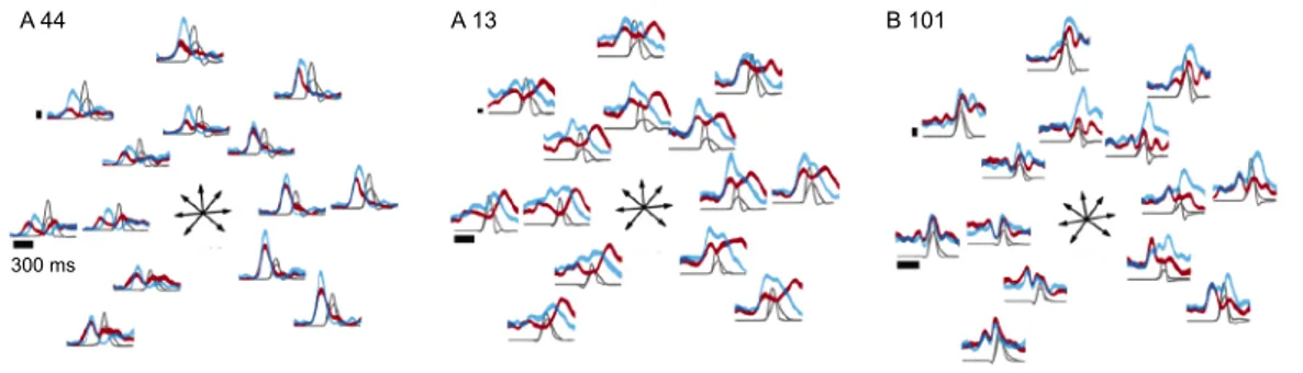
A classical example of in-vivo cortical recording is illustrated in Fig. 1.1. The data refer to the firing activity of a pyramidal cell from the visual area MT of a monkey [120], recorded while the animal is performing a random-dot motion task [21]. Neurons in area MT are known to encode the direction of motion of objects in the visual scene. As a consequence, the cell activity is presumably contributing to the monkey’s behavioural response.
The rastergram in Fig. 1.1ashows the firing activity of the cell across several identical rep-etitions of the task. Across the different trials, the spike trains display stereotyped modulations in the firing rate, which are elicited by a change in the stimulus coherence and luminance. A closer analysis within a smaller time window with almost flat firing rate, instead, reveals a finer temporal scale where the spike occurrence seems to be dominated by randomness (Fig. 1.1b).
Traditionally, the spike train variability has been quantified by looking at the fluctuations in the number of fired action potentials and in the time lag between two consecutive spikes. The inter-spike interval (ISI) histogram measured from in-vivo cortical recordings is typically broad (Fig. 1.1c), and its tail is compatible with an exponential decay [12]. The broadness of the ISI histogram can be measured in terms of the coefficient of variation, given by the ratio of the standard deviation to the mean of the distribution. The value of the coefficient of variation estimated from in-vivo recordings is high, and fluctuates between 0.5 and 1 [126].
The variability in the spike count is quantified instead by comparing the mean number of spikes computed within a fixed time window with the trial-to-trial variance. The values of the mean and the variance are typically found to be comparable (Fig. 1.1d). The curve can be fitted with a slightly super-linear relationship in all the brain areas that have been considered in the literature [43,144,22].
Both measures of variability point to a completely stochastic model of spike generation. A simple Poisson model, which assumes that spikes are fired at random from an underlying stationary firing rate, predicts both an exponential ISI histogram with unitary coefficient of variation and a linear increase of the variance with the mean of the spike count.
High levels of variability have been robustly observed across different animal preparations and across several brain areas [75,56], suggesting that what we perceive as noise could be an integrative and fundamental feature of the neural code. Experimental evidence thus quickly turned into fundamental theoretical questions, such as: is there any significance in the occur-rence and in the time position of a single spike, or is the information content redundantly stored in the form of average firing rates? Is variability a coding feature, or a constraint that the brain has to deal with?
1.1. Irregular firing in cortical networks
a. b.
c.
d.
Figure 1.1: Variability in a single neuron spiking activity: recordings from area MT of an alert monkey attending the random-dot motion task [21]. a. Rastergram and peri-stimulus time histogram. The same identical visual stimulus is presented across 210 different trials. Firing rate modulations are elicited by slow variations in the stimulus coherence and luminance. b.
Magnified view of the shaded region ina(from 360 to 460 ms), where the average firing rate is almost stationary. c. Inter-spike interval histogram. The solid line corresponds to the best exponential fit to the data. d.Variance in the spike count against the mean spike count. Every dot of the plot is measured in a different time window and from a restricted subset of trials. The best fit polynomial curve is displayed as solid line (y = x1.3), while the prediction from a stationary Poisson process is shown as dashed. Adapted from [120].
1.1.1 Irregular inputs, irregular outputs
Although a comprehensive understanding of the cortical code is far from being achieved, major progresses have been made in characterizing the possible mechanicistic sources which underlie the observed variability.
To begin with, neurons are complex and fragile biological devices. As a consequence, a fraction of variability is likely to be generated intrinsically during the input-output process which leads to the spike initiation. Possible sources of stochasticity arise from the finite number of open ion channels in the neuron membrane, from the thermal noise which acts on the charge carriers, or again from the low effectiveness of synaptic transmission [84,116,63].
Although such intrinsic sources of noise are likely to contribute, additional experimental evidences from in-vitro setups suggest that their role might be of minor relevance. When they are isolated from their afferent cells, indeed, neurons fairly reliably respond to slowly and fast modulated input currents [82,27].
a. b.
Figure 1.2: Poisson-like firing activity can emerge in model neurons which receive balanced excitatory and inhibitory input currents. a. Sample time traces of the membrane potential variable for a leaky integrate-and-fire model [53] of a cortical neuron. The neuron has mem-brane time constant τ = 10 (all units are arbitrary). The reset is at baseline, and the thresh-old membrane potential is at Vth = 10. The neuron receives a stationary excitatory input
current together with a stochastic contribution originating from 1000 excitatory and 1000 in-hibitory pre-synaptic Poisson spike trains. Top: the mean input value exceeds the threshold potential Vth. The membrane potential quickly climbs to the threshold value and thus quite
regularly generates spikes. Bottom: the mean input lays slightly below the threshold. In its sub-threshold dynamics, the membrane potential accumulates the Poisson noise, and spikes are emitted as a result of random fluctuations.b. Random network models where the strength of excitatory and inhibitory connections is correctly balanced admit a stable state where neu-rons asynchronously and irregularly emit action potentials. Rasterplot of the simulated spik-ing activity of 60 units from a larger network of N = 20000 leaky integrate-and-fire neurons. Model architecture as in [24].
are integrated in the cortical circuits is largely unknown. It is thus legitimate to hypothesise that neurons do not actively produce, but simply inherit, the noise which is already present at the level of their inputs. Cortical cells, indeed, integrate the action potentials which are gener-ated by several thousands of neighbouring cells. If one assumes that neighbouring neurons fire Poisson spikes, the total input current received by a single cortical neuron is purely stochastic, its mean and variance being determined by the firing rate of its pre-synaptic afferents.
Crucially, a model neuron which integrates an incoming noisy current can operate in a regime where the variability in the input is reflected in its output [142,53]. In order to obtain irregular outputs, it is critical to assume that the input contributions originating from excitatory and inhibitory pre-synaptic cells loosely balance each other [119,120].
In those conditions, the mean input is small and elicits solely sub-threshold responses in the post-synaptic membrane potential. Since the variance of the input does not vanish, however, the sub-threshold dynamics is dominated by noise, and spikes can be generated by random fluctuations of the membrane potential (Fig. 1.2a.). In this dynamical regime, the output of the neuron is far from saturation, a desirable feature which allows a wide range of firing rate responses [120].
The output variability can almost completely match the irregularity of the Poisson pro-cesses that the neuron receives as input [142]. The output firing rate ϕout depends on the
1.1. Irregular firing in cortical networks
statistics of the input current, or equivalently, on the average pre-synaptic firing rate ϕin. One
can write [125]:
ϕout= F (ϕin), (1.1)
where the function F incorporates both the details of the input connectivity structure and both the single-cell biophysical principles of the spike initiation.
If excitatory and inhibitory currents are correctly balanced, one can finally derive a more global picture where every neuron of the network receives and sends out noise. In a cortical assembly, indeed, every neuron acts both as input and as output. In the hypothesis that dif-ferent cells can be considered as statistically equivalent objects, a self-consistent network state requires [9,143,105]:
ϕ = F (ϕ). (1.2)
For a fixed function F , Eq. 1.2 can be used to determine the self-consistent firing rate ϕ at which every network unit is spiking.
Almost twenty years ago, rigorous mathematical analyses have been used to show that this self-consistent solution correspond to a stable collective state for the dynamics of random architectures of excitatory and inhibitory units [24, 145,11]. In this regime, the input cur-rent received by every neuron is dynamically maintained close to the threshold value thanks to the disordered structure of synaptic connections. As a consequence, spikes are driven by fluctuations and different neurons fire asynchronously (Fig. 1.2b). Extremely irregular spike trains emerge, even in absence of external sources of noise, because of the chaotic nature of the high-dimensional attractor underlying the dynamics.
To conclude, seminal studies have revealed that large, Poisson-like variability can sponta-neously emerge from the collective dynamics of completely deterministic model neurons that have been arranged in random architectures. As the mammalian cortex consists of large and intricate assemblies of neurons, it appears reasonable to hypothesize that collective network effects might significantly contribute to the total neural variability that has been measured from data.
1.1.2 Point-process and firing rate variability
If neurons in balanced cortical networks behave as Poisson spike generators, one could ratio-nally hypotesize that cortical cells mostly encode information through the firing rate variables which control their irregular spiking. While the network receives and processes its inputs, firing rates could be stationary or varying in time. As in Fig. 1.1 a, it is tempting to try to estimate the time course of a single cell firing rate by averaging the neural activity across many repetitions of the same measurement. Such approach, that has been widely adopted in the literature, in fact only returns a measure of the trial-averaged firing rate.
More recently, the necessity of considering inter-trial rate fluctuations as well has been pointed out [140,35,31]. Isolating the variability which derives from variations in the firing rates, in fact, can help build a more precise mapping between neural activity and behaviour, especially in tasks where the behavioural output is variable itself [34,33, 49,102]. In some cases, furthermore, the cortical response to behavioural stimuli might be not evident at the level of the average firing rate, while it might appear at the level of the amplitude of single-trial fluctuations [35]. Finally, it has been suggested that a principled analysis of rate variability could help distinguishing between alternative computational models for cortical dynamics [35,
When the neural activity is averaged across trials, the variability in the firing rates, or
gain variability, is washed out together with the variability associated with the Poisson spike
generation, also referred to as point-process variability. Both sources of irregularity, on the other hand, are integrated together when standard variability measures are applied, like the Fano factor for the spike count and the coefficient of variation for the inter-spike intervals.
The two contributions can be disentangled by considering doubly stochastic models of spike initiation [35, 31, 56]. In those frameworks, spikes are emitted at random from an underlying time-varying firing rate. Crucially, the rate consists of a deterministic, stimulus-driven component ν, which is frozen across different trials, and of a trial-dependent gain G which enters multiplicatively [56]:
ϕ = Gν. (1.3)
Introducing the gain variable G allows to largely improve the precision of the fit to the neural data recorded from several distinct cortical regions [56]. As shown in Fig. 1.3a, fur-thermore, assuming a multiplicative dependence of the rate on the gain predicts an excess of variance which resembles the super-Poisson variability which has been long observed in the literature [126,120,140]. The time traces of the gain that are directly inferred from the neural data display indeed large trial-to-trial variability, which can be measured in terms of its coeffi-cient of variation (Fig. 1.3b). Larger firing rate variability is typically observed in areas which are higher in the cortical hierarchy.
The gain auto-correlogram in Fig. 1.3c reveals that rate fluctuations are typically slow, with relaxation time scales which can last up to several minutes. On average, the cortical relaxation time scales follow a precise hierarchical ordering, with sensory and prefrontal areas exhibiting, respectively, shorter and longer time constants [92].
A significative fraction of the firing rate variability appears to be shared across neurons covering wide cortical areas, and is likely to importantly contribute to the correlation patterns between pairs of cells [56,35]. This observation is agreement with the long-standing hypoth-esis that rate fluctuations derive from modulations in the excitability controlled by top-down signals linked to arousal and attention [140].
On the other hand, the shared component of rate variability seems to be restricted to rel-atively fast fluctuations [56]. The tails of the auto-correlation function which correspond to slow fluctuations, indeed, are absent in the cross-correlogram measured within pairs of differ-ent neurons (Fig. 1.3c). Single neurons thus seem to develop local and extremely slow firing rate modulations, a scenario which is more difficult to reconcile with a top-down modulatory hypothesis. Fast and slow firing rate modulations could thus originate from distinct generating mechanisms.
1.2 Chaotic regimes in networks of firing rate units
One recent hypothesis suggests that, similarly to point-process variability, slow and local firing rate modulations could be produced intrinsically through the recurrent circuitry of the cortex [66]. A convenient network model, which spontaneously sustains slowly fluctuating dynamical regimes, was found almost thirty years ago in a seminal work by Sompolinsky and colleagues [127].
In this study, the collective behaviour of large disordered networks of non-linear units is examined (Fig. 1.4a). Every node in the network is characterized by a continuous state variable, whose dynamics obeys a smooth evolution law. At every node, the activation variable
1.2. Chaotic regimes in networks of firing rate units a. b. c. LGN V1 V2 MT
Figure 1.3: Spike trains from cortical in-vivo recordings can be parsimoniously described by a doubly stochastic model, where the firing rate across different trials contains both a frozen and a variable component (Eq. 1.3). a. Spike count variance-to-mean relation for a single V1 neuron stimulated with grating stimuli drifting in different directions. The prediction from the doubly stochastic model fitted to data is displayed in blue. The prediction from a simple Poisson model is shown in black. Means and variances were computed over 125 repetitions of each stimulus direction. b. Trial-to-trial variability of the gain variable inferred from the doubly stochastic model, quantified through its coefficient of variation. The full distribution is obtained by performing the analysis on different time windows. Different colors refer to different data sets, recorded from different cortical areas in the visual pathway. c. Temporal structure of the inferred gain, measured in four different data sets and averaged across many recorded cells. Left: auto-correlation, right: cross-correlation. Adapted from [56].
xi, loosely interpreted as the total current entering the unit, is non-linearly transformed into
an output ϕ(xi). Critically, the network architecture is random, i.e. the pairwise coupling
parameters are drawn from a Gaussian probability distribution.
It was found that the overall strength of the network connectivity structure controls the appearance of smooth chaotic fluctuations from a silent network regime. At the bifurcation point, an extensive number of eigenvectors become unstable. Network activity is then push-pulled in many different random directions, resulting in irregular and uncorrelated fluctuations with complex spatio-temporal profiles (Fig. 1.4b). In this irregular state, an explicit calculation of the Lyapunov exponents indicates that fluctuations have exponentially short memory of their past history. As the dynamics is fully deterministic, network activity is formally chaotic. A second attractive feature of this network model is the rich variety of activity time scales that it can support. The time scale of chaotic fluctuations is indeed controlled by the main
a. b.
Figure 1.4: Irregular and smooth fluctuations spontaneously emerge as collective phe-nomenon in networks of randomly coupled non-linear units. a. A random network: activ-ity in each node is described by a continuous variable xi(t)which obeys a smooth temporal
evolution law. The non-linear input-output transformation performed by single units is mod-eled through the activation function ϕ(x). b. Sample of chaotic activity in finite networks: temporal evolution of the activation variable xifor six randomly selected unit. Activity traces
fluctuate irregularly around zero.
parameter of the system, i.e. the overall connectivity strength. Close to the critical point, the time decay of fluctuations sharply increases; it formally diverges in the limit of infinite networks size.
Although the network dynamics in [127] can be formally mapped into a standard firing rate model [42, 151], whether similar irregular states are expected to appear in biologically-motivated models of cortical networks has been a long-standing question. Indeed, while this model captures the essence of the non-linear input-output transformation taking place in real neurons, it lacks the elementary features that would enable a direct comparison with other more realistic networks models. For many years, very little effort has been devoted to build and explore such a link.
In the last few years, this class of models has been attracting increasing attention. As already discussed, this renewed interest can be partially attributed to the recent improvement in the neural recordings techniques, that have allowed to systematically disentangle multiple levels of variability in the neural data.
A second significant contribution has come from the recent advances in the research field at the frontier between neuroscience and machine learning. The model from [127] is indeed widely adopted in novel lines of research which explore learning and plasticity mechanisms in recurrent network models [67,132,73,85,138]. Because of the complex temporal dependen-cies that are intrinsically generated by recurrent circuits, training recurrent neural networks has been historically a cumbersome task. A variety of novel training strategies have only re-cently allowed to efficiently build artificial computational models which can solve elaborate spatio-temporal tasks. Apart from being attractive tools for the theoretical and machine learn-ing communities, trained networks have been combined with neural recordlearn-ings to get valuable insights on the dynamics and coding principles of the cortex [83,15,100,128,88].
Despite their efficacy and prediction power, trained neural networks are in most of the cases black box models designed on obscure – and hard to capture – dynamical principles [13,133]. Most of the modelling efforts consecrated to understanding large circuits dynamics
1.3. Outline of the work
have been focusing indeed on completely random network architectures [24,145,127], where the relationship between connectivity and dynamics can be understood in great detail. On the contrary, a rigorous understanding of non-random computational networks presents, from a theoretical point of view, several novel challenges which still need to be addressed. As a result, what are the dynamical mechanisms underlying computations in trained networks – and how variability is characterized in computational circuit models – are still largely unsolved theoretical questions.
1.3
Outline of the work
In this thesis, we investigate how intrinsically generated variability can be integrated in more realistic models of cortical networks which can serve as elementary units of computation. The dissertation collects the results of three years of work and consists of three main parts.
I. In the first part, we take direct inspiration from the original work in [127] and we design a random network model which includes several additional constraints directly moti-vated by biology. We consider a network architecture which respects Dale’s law: every unit in the network can either excite or inhibite his neighbours. Moreover, we include more realistic, positively defined, current-to-rate activation functions. We show that rate fluctuations appear in strongly coupled excitatory-inhibitory architectures, and we study how variability depends on further biophysical restrictions, like firing-rate saturation, heterogeneity in the connectivity and spiking noise. A constrained network model allows for a neater comparison with the more realistic networks of spiking units that have been traditionally adopted as models for irregular activity in cortical circuits. In this perspective, we show that our simple rate description can be used to help understanding the more complex dynamics generated in strongly inter-connected networks of leaky integrate-and-fire neurons, where classical mean field approaches fail to pro-vide a good description of spiking activity [95].
II. In the second part, we turn to a simple computational architecture, which includes a random network together with a single feedback signal. Such elementary connectivity scheme has been successfully exploited in different training setups [67,132]. Since the network con-nectivity is not far from being completely random, we show that the classical mathematical tools developed for the analysis of large disordered systems can be fruitfully applied to this sce-nario. We perform a systematic analysis of a network model designed to behave as a generator of arbitrary periodic patterns. Consistently with our theory, we show that training perfor-mance significantly improves in highly disordered architectures. When the random compo-nent of the connectivity is strong, in fact, the intrinsic heterogeneity prevents network activity from synchronizing. Learning can thus take advantage of a widely decorrelated set of neural activitiy from which the desired output pattern can be solidly reconstructed.
III. Random networks with a single feedback unit can be more generally thought as novel recurrent architectures where the global connectivity structure consists of the sum of a random and of a unit rank structured term. More in general, the idea that neural computa-tions in large recurrent networks only rely on low-dimensional connectivity structures is widely shared across several training frameworks [65,67,132,20,48]. Motivated by this observation, in the third part of this dissertation we explore the dynamics of large random networks
per-turbed by weak, low-dimensional connectivity structures. We find that rank one and rank two connectivity structures that are generated by high-dimensional random vectors can generate a rich variety of irregular and heterogeneous dynamical regimes. The knowledge of the stable states of the dynamics allows to easily design partially structured models which can perform simple tasks. In the resulting computational models, our theoretical framework allows to pre-dict the variability properties and the largest relaxation time scales of the dynamics. It further permits to neatly interpret the low-dimensional evolution of the population activity in terms of the few structured directions that are specified by the network architecture and inputs.
Part I
intrinsically-generated
fluctuations in random networks
of excitatory-inhibitory units
Summary of Chapters 2 - 3 - 4
Recurrent networks of non-linear units display a variety of dynamical regimes depending on the structure of their synaptic connectivity. A particularly remark-able phenomenon is the appearance of strongly fluctuating, chaotic activity in networks of deterministic, but randomly connected rate units. How this type of intrinsically generated fluctuations appears in more realistic networks of spiking neurons has been a long standing question. The comparison between rate and spiking networks has in particular been hampered by the fact that most previous studies on randomly connected rate networks focused on highly simplified models, in which excitation and inhibition were not segregated and firing rates fluctuated symmetrically around zero because of built-in symmetries.
To ease the comparison between rate and spiking networks, we investigate the dynamical regimes of sparse, randomly-connected rate networks with segregated excitatory and inhibitory populations, and firing rates constrained to be positive. Extending the dynamical mean field theory, we show that network dynamics can be effectively described through two coupled equations for the mean activity and the auto-correlation function. As a consequence, we identify a new signature of intrinsically generated fluctuations on the level of mean firing rates. We more-over found that excitatory-inhibitory networks develop two different fluctuating regimes: for moderate synaptic coupling, recurrent inhibition is sufficient to stabi-lize fluctuations; for strong coupling, firing rates are stabistabi-lized solely by the upper bound imposed on activity. These results extend to more general network archi-tectures, and to rate networks receiving noisy inputs mimicking spiking activity. Finally, we show that signatures of those dynamical regimes appear in networks of integrate-and-fire neurons.
A substantial fraction of this part of the dissertation is adapted from the manuscript: Intrinsically-generated fluctuating activity in excitatory-inhibitory
net-works by F. Mastrogiuseppe and S. Ostojic, PLoS Computational Biology (2017)
Dynamical Mean Field description of
excitatory-inhibitory networks
2
In the first part of this dissertation, we study how the transition to a chaotic, slowly fluctuating dynamical regime, which was first observed in [127], translates to more realistic network mod-els. We design a non-linear firing rate network which includes novel mathematical contraints motivated by biology, and we quantitatively address its spontaneous dynamics.
If the synaptic coupling is globally weak, firing rate networks can be described with the help of standard approaches from dynamical systems theory, like linear stability analysis. However, in the strong coupling regime, a rigorous description of self-sustained fluctuations can be de-rived only at the statistical level. To this end, we adopt and extend the theoretical framework first proposed in [127], which provides an adequate description of irregular temporal states. In such approach, irregular trajectories are thought as random processes sampled from a con-tinuous probability distribution, whose first two momenta can be computed self-consistently [127]. This technique, commonly referred to as Dynamical Mean Field (DMF) theory, has been inherited from the study of disordered systems of interacting spins [40], and provides a powerful and flexible tool for understanding dynamics in disordered rate networks.
In this chapter, we adapt this approach to the study of more realistic excitatory-inhibitory network models. We derive the mean field equations which will become the central core of the analysis which is carried out in details in the rest of part I. To begin with, we review the methodology of DMF, and we present the results that such theory implies for the original, highly symmetrical model. This first section is effectively a re-interpretation of the short paper by [127]. In the second section, we introduce and motivate the more biologically-inspired model that we aim at studying, and we show that an analogous instability from a fixed point to chaos can be predicted by means of linear stability arguments. In order to provide an adequate self-consistent description on the irregular regime above the instability, we extend the DMF framework to include non-trivial effects due to non-vanishing first-order statistics.
2.1
Transition to chaos in recurrent random networks
The classical network model in [127] is defined through a non-linear continuous-time dynam-ics which makes it formally equivalent to a traditional firing rate model [151,42]. Firing rate models are meant to provide a high-level description of circuit dynamics, as spiking activity is averaged over one or more degrees of freedom to derive a simpler description in terms of smooth state variables. From a classical perspective, firing rate units provide a good descrip-tion of the average spiking activity in small neural populadescrip-tions. Equivalently, they can well approximate the firing of single neurons if the synaptic filtering time-scale is large enough. Although in this chapter we don’t focus on any specific interpretation, a sloppy terminology where the words unit and neuron are used indifferently will be adopted.
The state of each unit in the network is described through an activation variable xiwhich is
commonly interpreted as the net input current entering the cell. The current-to-rate transfor-mation that is performed in spiking neurons is modeled through a monotonically increasing function ϕ, such that the variable ϕ(xi)represents the instantaneous output firing rate of the
unit.
As the network consists of many units (i = 1, ..., N ), the current entering neuron i in-cludes many contributions, whose values are proportional to the firing rate of the pre-synaptic neurons. The strength of the synapse from neuron j to neuron i is modeled through the con-nectivity parameter Jij. The coupled dynamics obey the following temporal evolution law:
˙ xi(t) =−xi(t) + N ∑ j=1 Jijϕ(xj(t)). (2.1)
The first contribution on the r.h.s. is a leak term, which ensures the activation variables xi
decays back to baseline in absence of any forcing current. The incoming contributions from other units in the network sum linearly. Note that we have rescaled time to set the time constant to unity.
In the paper by [127], the authors focus on a random all-to-all Gaussian connectivity (Fig. 2.1a). We thus have Jij = gχijwith χij ∼ N (µ = 0, σ2 = 1/N ). Such scaling for the
variance ensures that single units experience finite input fluctuations even in the limit of very large networks. The parameter g controls the global strength of synaptic coupling. As neurons can make both excitatory and inhibitory connections, this connectivity scheme does not respect Dale’s law. The activation function is a symmetric sigmoid (ϕ(x) = tanh(x)), which takes positive and negative values. In the original network, furthermore, neither constant nor noisy external inputs are considered.
As we will show in the next sections, all those elements together result in an extremely simplified dynamics, where the transition to chaos can be only measured at the level of the second-order statistics of the network activity distribution.
2.1.1 Linear stability analysis
To begin with, we notice that the model admits an homogeneous stationary solution for which the network is completely silent: x0
i = 0∀i. For a fixed, randomly chosen connectivity matrix,
the network we consider is fully deterministic, and can therefore be examined using standard dynamical system techniques [131]. We thus derive a first intuitive picture about the network dynamics by evaluating the linear stability of the homogeneous fixed point.
2.1. Transition to chaos in recurrent random networks
a. b. c.
d. e.
Figure 2.1: Linear stability analysis and transition to chaos in all-to-all Gaussian networks with symmetric activation function [127]. a. The Gaussian connectivity matrix gχij. b-c.
Stationary regime: g = 0.8. Inb: eigenspectrum of the stability matrix Sij for a simulated
network of N = 2000 units. In good agreement with the circular law prediction, the eigen-values lie in a compact circle of radius g (continuous black line). Dashed line: instability boundary. Inc: sample of simulated activity for eight randomly chosen units. d-e. Chaotic regime: g = 1.2. Same figures as inb-c.
The linear response of the system when pushed away from the fixed point can be studied by tracking the time evolution of a solution in the form: xi(t) = x0 + δxi(t). Close to the
fixed point, the function ϕ(x) can be expanded up to the linear order in δxi(t). This results
in a system of N coupled linear differential equations, whose dynamical matrix is given by:
Sij = ϕ′(0)gχij− δij. Note that here ϕ′(0) = 1.
As a result, the perturbation δxi(t)will be re-absorbed ifRe(λi) < 1for all i, λibeing
the ith eigenvalue of the asymmetric random matrix gχij. We are thus left with the problem
of evaluating the eigenspectrum of a Gaussian random matrix. If one focuses on very large networks, the circular (or Girko’s) law can be applied [54,136]: the eigenvalues of gχij lie in
the complex plane within a circular compact set of radius g. Although its prediction is exact only in the thermodynamic limit (N → ∞), the circular law also reasonably well approximate the eigenspectrum of finite random matrices.
We derive that, at low coupling strength (g < 1), the silent fixed point is stable (Fig. 2.1
b-c). More than this, x0= 0is a global attractor, as Sijis a contraction [146]. Numerical
sim-ulations confirm that, in this parameter region, network activity settles into the homogeneous fixed point. For g > 1, the fixed point is unstable, and the network exhibits ongoing dynamics in which single neuron activity fluctuates irregularly both in time and across different units (Fig. 2.1d-e). As the system is deterministic, these fluctuations are generated intrinsically by strong feedback along unstable modes, which possess a random structure inherited from the random connectivity matrix.
2.1.2 The Dynamical Mean Field theory
The non-stationary regime cannot be easily analyzed with the tools of classical dynamical sys-tems. To this end, the authors in [127] adopted a mean field approach to develop an effective statistical description of network activity. In this section, we propose a review of such tech-nique; our analysis is based on [127] and subsequent works [99,141,89].
Rather than attempting to describe single trajectories, the main idea is to focus on their statistics, which can be determined by averaging over different initial conditions, time and the different instances of the connectivity matrix. Dynamical Mean Field (DMF) acts by replacing the fully deterministic interacting network by an equivalent stochastic system. More specifically, as the interaction between units∑jJijϕ(xj)consists of a sum of a large number of
terms, it can be replaced by a Gaussian stochastic process ηi(t). Such a replacement provides
an exact mathematical description under specific assumptions on the chaotic nature of the dynamics [16,90] in the limits of large network size N . In this thesis, we will treat it as an approximation, and we will assess the accuracy of this approximation by comparing the results with simulations performed for fixed N .
Replacing the interaction terms by Gaussian processes transforms the system into N iden-tical Langevin-like equations:
˙
xi(t) =−xi(t) + ηi(t). (2.2)
As ηi(t)is a Gaussian noise, each trajectory xi(t)emerges thus as a Gaussian stochastic process.
As we will see, the stochastic processes corresponding to different units become uncorrelated and statistically equivalent in the limit of a large network, so that the network is effectively described by a single process.
Within DMF, the mean and correlations of this stochastic process are determined self-consistently, by requiring that averages over ηi(t)be identical to averages over time, instances
of the connectivity matrix and initial conditions in the original system. Both averages will be indicated with []. For the mean, we get:
[ηi(t)] = g[ N ∑ j=1 χijϕ(xj(t))] = g N ∑ j=1 [χij][ϕ(xj(t))] = 0 (2.3)
as [χij] = 0. In the second equality, we assumed that activity of different units decorrelates in
large networks; in particular, that activity of unit j is independent of its outgoing connections
Jij. As we will show in few lines, this assumption is self-consistent. In the mathematical
literature, it has been referred to as local chaos hypothesis [8,52,90]. The second-order statistics of the effective input gives instead:
[ηi(t)ηj(t + τ )] = g2[ N ∑ k=1 χikϕ(xk(t)) N ∑ l=1 χjlϕ(xl(t + τ ))] = g2 N ∑ k=1 N ∑ l=1 [χikχjl][ϕ(xk(t))ϕ(xl(t + τ ))]. (2.4)
As [χikχjl] = δijδkl/N, cross-correlations vanish, while the auto-correlation results in:
2.1. Transition to chaos in recurrent random networks
We will refer to the firing rate auto-correlation function [ϕ(xi(t))ϕ(xi(t + τ ))]as C(τ ).
Con-sistently with our starting hypothesis, the first- and the second-order statistics of the Gaussian process are uncorrelated from one unit to the other.
Once the probability distribution of the effective input has been characterized, we derive a statistical description of the network activity in terms of the activation variable xi(t)by solving
the Langevin equation in Eq. 2.2.
Trivially, the first-order statistics of xi(t)and ηi(t)asymptotically coincide, so that the
mean input always vanishes. In order to derive the auto-correlation function ∆(τ ) = [xi(t)xi(t+
τ )], we derive twice with respect to τ and we combine Eqs. 2.2 and 2.5 to get the following time evolution law:
¨
∆(τ ) = ∆(τ )− g2C(τ ). (2.6)
We are thus left with the problem of writing down an explicit expression for the firing rate auto-correlation function C(τ ). To this aim, we write x(t) and x(t + τ ) as Gaussian variables which obey [x(t)x(t + τ )] = ∆(τ ) and [x(t)2] = [x(t + τ )2] = ∆
0, where we defined the input variance ∆0= ∆(τ = 0). One possible choice is:
x(t) =√∆0− |∆(τ)|x1+ √ |∆(τ)|z x(t + τ ) =√∆0− |∆(τ)|x2+sgn(∆(τ )) √ |∆(τ)|z (2.7)
where x1, x2 and z are Gaussian variables with zero mean and unit variance. For reasons which will become clear in few steps, we focus on the case ∆(τ ) > 0. Under this assumption, the firing rate auto-correlation function can be written as:
C(τ ) = ∫ Dz [∫ Dxϕ(√∆0− ∆(τ)x + √ ∆(τ )z) ]2 (2.8)
where used the short-hand notation:∫ Dz =∫−∞+∞e− z
2 2
√
2πdz.
From a technical point of view, Eq. 7.61 is now a second-order differential equation, whose time evolution depends on its initial condition ∆0. This equation admits different classes of solutions which are in general hard to isolate in an explicit form. Luckily, we can reshape our problem into a simpler, more convenient formulation.
Isolating the solutions We observe that Eq. 7.61 can be seen as analogous to the equation of motion of a classical particle in a one-dimensional potential:
¨
∆ =−∂V (∆, ∆0)
∂∆ (2.9)
The potential V (∆, ∆0)is given by an integration over ∆:
V (∆, ∆0) =− ∫ ∆ 0 d∆′[∆′− g2C(∆′, ∆0) ] . (2.10)
One can check that this results in:
V (∆, ∆0) =− ∆2 2 + g 2 ∫ Dz [∫ DxΦ(√∆0− ∆x + √ ∆z) ]2 (2.11)
a. b.
Figure 2.2: Shape of the potential V (∆, ∆0)for different initial conditions ∆0. a. Weak copling regime: g < gC.b. Strong coupling regime: g > gC.
where Φ(x) =∫−∞x ϕ(x′)d x′. In the present framework, Φ(x) = ln(cosh(x)).
In absence of external noise, the initial condition to be satisfied is ˙∆(τ = 0) = 0, which implies null kinetic energy for τ = 0. A second condition is given by: ∆0 >|∆(τ)| ∀τ. The solution ∆(τ ) depends on the initial value ∆0, and is governed by the energy conservation law:
V (∆(τ = 0), ∆0) = V (∆(τ =∞), ∆0) + 1
2∆(τ =˙ ∞)
2 (2.12)
The stationary points and the qualitative features of the ∆(τ ) trajectory depend then on the shape of the potential V . We notice that for the symmetric model from [127], the derivative of the potential in ∆ = 0 always vanishes, suggesting a possible equilibrium point. The full shape of V is determined by the values of g and ∆0. In particular, a critical value gC exists
such that:
• when g < gC, the potential has the shape of a concave parabola centered in ∆ = 0
(Fig. 2.2 a). The only bounded solution is ∆ = ∆0= 0;
• when g > gC, the potential admits different qualitative configurations and an infinite
number of different ∆(τ ) trajectories. In general, the motion in the potential will be oscillatory (Fig. 2.2 b).
We conclude that, in the weak coupling regime, the only acceptable solution is centered in 0 and has vanishing variance. In other terms, in agreement with our linear stability analysis, we must have xi(t) = 0∀t.
In the strong coupling regime, we observe that a particular solution exists, for which ∆(τ ) decays to 0 as τ → ∞. In this final state, there is no kinetic energy left. For this particular class of solutions, Eq. (2.12) reads:
V (∆0, ∆0) = V (0, ∆0). (2.13) More explicitly, we have:
∆20 2 = g 2 {∫ DzΦ2(√∆ 0z)− (∫ DzΦ(√∆0z) )2} . (2.14)
2.2. Fast dynamics: discrete time evolution
In the following, we will often use the compact notation: ∆20
2 = g
2{[Φ2]− [Φ]2}. (2.15) A monotonically decaying auto-correlation function implies a dynamics which loses mem-ory of its previous states, and is compatible with a chaotic state. In the original study by Sompolinsky et al. [127], the average Lyapunov exponent is computed. It is shown that the monotonically decreasing solution is the only self-consistent one, as the correspondent Lya-punov exponent is positive.
Once ∆0 is computed through Eq. 2.15, its value can be injected into Eq. 7.61 to get the time course of the auto-correlation function. The decay time of ∆(τ ), which depends on g, gives an estimation of time scale of chaotic fluctuations. As the transition in gC is smooth,
the DMF equations can be expanded around the critical coupling to show that such time scale diverges when approaching the transition from above. Very close to g = gC, the network can
thus support arbitrarily slow spontaneous activity.
Numerical inspection of the mean field solutions suggest that, as it has been predicted by the linear stability analysis, gC = 1(Fig. 2.3 b). This can be also rigorously checked by
imposing that, at the transition point, the first and the second derivative of the potential vanish in ∆ = 0.
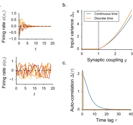
To conclude we found that, above g = 1, the DMF predicts the emergence of chaotic trajectories which fluctuate symmetrically around 0. In the large network limit, different tra-jectories behave as totally uncoupled processes. Their average amplitude can be computed numerically as solution of the non-linear self-consistent equation in 2.15.
2.2 Fast dynamics: discrete time evolution
As a side note, we briefly consider a closely related class of models which has been extensively adopted in the DMF literature. In this formulation, the dynamics is given by a discrete time update: xi(t + 1) = N ∑ j=1 Jijϕ(xj(t)) (2.16)
As there are no leak terms, fluctuations in the input current occur on an extremely fast time-scale (formally, within one time step). All the other elements of the model, including Jij and
ϕ(x), are taken as in [127].
This discrete-time formulation has been used, for instance, in the first attempts to exploit random network dynamics for machine learning purposes [67]. It has also been adopted in several theoretically oriented studies, as analysing fast dynamics has two main advantages: mean field descriptions are easier to derive [89, 141, 30], and, in finite-size networks, the quasi-periodical route to chaos can be directly observed [46,30,4].
While finite size analysis falls outside the scope of this dissertation, we briefly review how the mean field equations adapt to discrete-time networks and how this description fits in the more general DMF framework.
Similar to the continuous-time case, the discrete-time dynamics admits an homogeneous fixed point in x0 = 0. Furthermore, as it can be easily verified, the linear stability matrix of this stationary state coincides with Sij = gχij− δij, so that an instability occurs in g = 1. In
a. b.
c.
Figure 2.3: Discrete-time dynamics in random neural networks. a. Sample of simulated activity: time traces for eight randomly chosen units in the static (top) and in the chaotic regime (bottom). b. Bifurcation diagram for the second-order statistics ∆0 as a function of the coupling strength parameter g. The value of ∆0 is evaluated by solving iteratively the DMF equations for continuous- (Eq. 2.15) and discrete-time (Eq. 2.20) networks. Vertical line: critical coupling in gC = 1. c.Temporal shape of the auto-correlation function for fixed
g = 1.3. The time scale of discrete-time dynamics is set arbitrarily.
order to analyze dynamics beyond the instability, we apply DMF arguments. When defining the effective input ηi(t) =
∑N
j=1Jijϕ(xj(t)), fast dynamics will translate in the following
simple update rule:
xi(t + 1) = ηi(t) (2.17)
where, at each time step, xi is simply replaced by the stochastic effective input. As a
con-sequence, by squaring and averaging over all the sources of disorder, we find that the input current variance obeys the following time evolution:
∆0(t + 1) = [ηi2(t)] = g2[ϕ2(t)]. (2.18)
In the last equality, we used the self-consistent expression for the second-order statistics of
ηi, which can be computed as in the continuous-time case, yielding to the same result. By
expressing x(t) as Gaussian variable, the evolution law for ∆0can be made explicit: ∆0(t + 1) = g2
∫
Dzϕ2(√∆
0(t)z). (2.19)
At equilibrium, the value of ∆0 satisfies the fixed-point condition: ∆0 = g2
∫
Dzϕ2(√∆
2.3. Transition to chaos in excitatory-inhibitory neural networks
As it can be easily checked, this equation is satisfied for ∆0 = 0when g < 1, while it admits a nontrivial positive solution above gC = 1, corresponding to a fast chaotic phase (Fig. 2.3 b).
The solution that we derive from solving Eq. 2.20 does not coincide exactly with the so-lution we obtained in the case of continuous-time networks, although they share many quali-tative features (Fig. 2.3b). In contrast to discrete-time units, neurons with continuous-time dynamics act as low-pass filters of their inputs. For this reason, continuous-time chaotic fluc-tuations are characterized by a slower time scale (Fig. 2.3c) and a smaller variance ∆0(Fig. 2.3
b).
We conclude this paragraph with a technical remark: our new equation for ∆0(Eq. 2.20) coincides with the general expression for stationary solutions in continuous-time networks. The latter can be derived from the continuous-time DMF equation ¨∆(τ ) = ∆(τ )− g2C(τ )
by setting x(t) = x(t + τ ) and thus ¨∆(τ ) = 0. From the analysis we just carried out, we con-clude that the general stationary solution for continuous-time networks admits, together with the homogeneous fixed point, a non-homogeneous static branch for g > 1. As it is charac-terized by positive Lyapunov exponents, this solution is however never stable for continuous-time networks. This sets a formal equivalence between chaotic discrete-continuous-time and stationary continuous-time solutions which does not depend on the details of the network model. For this reason, it will return back several times within the body of this dissertation.
2.3 Transition to chaos in excitatory-inhibitory neural networks
As widely discussed in Chapter 1, network models which spontaneously sustain slow and local firing rate fluctuations are of great interest in the perspective of understanding the large, super-Poisson variability observed from in-vivo recordings [120,56].Furthermore, the random network model in [127] has been adopted in many training frameworks as a proxy for the unspecialized substrate on which plasticity algorithms can be applied. The original computational architecture from Jaeger [67], know as echo-state machine, adopts the variant of the model characterized by discrete-time dynamics [89,30]. In later years, several training procedures have been designed for continuous-time models as well [132,73,
28].
A natural question we would like to address is whether actual cortical networks exhibit dynamical regimes which are analogous to rate chaos.
The classical network model analyzed in [127] and subsequent studies [132, 73, 99, 6,
7, 130] rely on several simplifying features that prevent a direct comparison with more bi-ologically constrained models such as networks of spiking neurons. In particular, a major simplification is a high degree of symmetry in both input currents and firing rates. Indeed, in the classical model the synaptic strengths are symmetrically distributed around zero, and excitatory and inhibitory neurons are not segregated into different populations, thus violating Dale’s law. The current-to-rate activation function is furthermore symmetric around zero, so that the dynamics are symmetric under sign reversal. As a consequence, the mean activity in the network is always zero, and the transition to the fluctuating regime is characterized solely in terms of second order statistics.
To help bridge the gap between the classical model and more realistic spiking networks [24,95], recent works have investigated fluctuating activity in rate networks that include ad-ditional biological constraints [95, 69, 58], such as segregated excitatory-inhibitory popula-tions, positive firing rates and spiking noise [69]. In general excitatory-inhibitory networks,
the DMF equations can be formulated, but are difficult to solve, so that these works focused mostly on the case of purely inhibitory networks. These works therefore left unexplained some phenomena observed in simulations of excitatory-inhibitory spiking and rate networks [95], in particular the observation that the onset of fluctuating activity is accompanied by an elevation of mean firing rate.
Here we investigate the effects of excitation on fluctuating activity in inhibition-dominated excitatory-inhibitory networks [142,91,3,111,60,61]. To this end, we focus on a simplified network architecture in which excitatory and inhibitory neurons receive statistically identical inputs [24]. For that architecture, dynamical mean field equations can be fully solved.
2.3.1 The model
We consider a large, randomly connected network of excitatory and inhibitory rate units. Sim-ilarly to [127], the network dynamics are given by:
˙ xi(t) =−xi(t) + N ∑ j=1 Jijϕ(xj(t)) + Ii. (2.21)
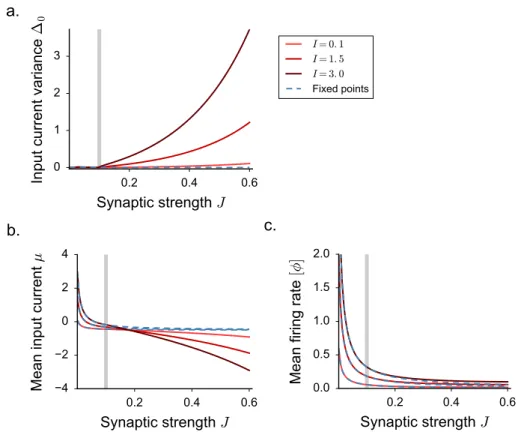
In some of the results which follow, we will include a fixed or noisy external current Ii. The
function ϕ(x) is a monotonic, positively defined activation function that transforms input currents into output activity.
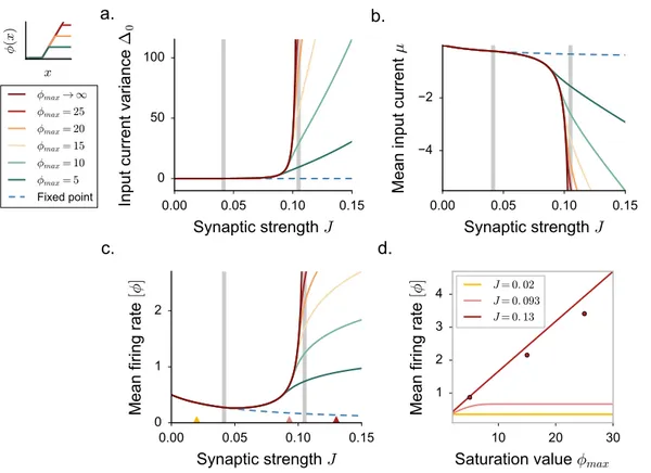
For the sake of simplicity, in most of the applications we restrict ourself to the case of a threshold-linear activation function with an offset γ. For practical purposes, we take:
ϕ(x) = 0 x <−γ γ + x −γ ≤ x ≤ ϕmax− γ ϕmax x > ϕmax− γ (2.22)
where ϕmaxplays the role of the saturation value. In the following, we set γ = 0.5.
We focus on a sparse, two-population synaptic matrix identical to [24,95]. We first study the simplest version in which all neurons receive the same number C ≪ N of incoming connections (respectively CE = f C and CI = (1− f)C excitatory and inhibitory inputs).
More specifically, here we consider the limit of large N while C (and the synaptic strengths) are held fixed [9,24]. We set f = 0.8.
All the excitatory synapses have strength J and all inhibitory synapses have strength−gJ, but the precise pattern of connections is assigned randomly (Fig. 2.4a). For such connectivity, excitatory and inhibitory neurons are statistically equivalent as they receive statistically identi-cal inputs. This situation greatly simplifies the mathematiidenti-cal analysis, and allows us to obtain results in a transparent manner. In a second step, we show that the obtained results extend to more general types of connectivity.
Our analysis largely builds on the methodology that we have been reviewing in the previous section for the case of the simpler network as in [127].
2.3.2 Linear stability analysis
As the inputs to all units are statistically identical, the network admits a homogeneous fixed point in which the activity is constant in time and identical for all units, given by:
2.3. Transition to chaos in excitatory-inhibitory neural networks
a. b. c.
d. e.
Figure 2.4: Linear stability analysis and transition to chaos in excitatory-inhibitory networks with threshold-linear activation function.a. The sparse excitatory-inhibitory connectivity ma-trix Jij. b-c. Stationary regime: J < J0. Inb: eigenspectrum of the stability matrix Sij for
a simulated network of N = 2000 units. In good agreement with the circular law prediction, the eigenvalues lie in a compact circle of approximated radius J√CE + g2CI (black
contin-uous line). Black star: eigenspectrum outlier in J(CE − gCI) < 0. Dashed line: instability
boundary. Inc: sample of simulated activity for eight randomly chosen units. d-e. Chaotic regime: J > J0. Same figures as inb-c.
The linear stability of this fixed point is determined by the eigenvalues of the matrix Sij =
ϕ′(x0)Jij.
In the limit of large networks, the eigenspectrum of Jij consists of a continuous part that
is densely distributed in the complex plane over a circle of radius J√CE+ g2CI, and of
a real outlier given by the effective balance of excitation and inhibition in the connectivity
J (CE − gCI)(Fig. 2.4b-d) [98,54,136,135]. We focus here on an inhibition-dominated
network corresponding to g > CE/CI. In this regime, the real outlier is always negative and
the stability of the fixed point depends only on the continuous part of the eigenspectrum. The radius of the eigenspectrum disk, in particular, increases with the coupling J, and an instability occurs when the radius crosses unity. The critical coupling J0is given by:
ϕ′(x0)J0 √
CE+ g2CI = 1 (2.24)
where x0depends implicitly on J through Eq. 2.23 and the gain ϕ′(x)is in general finite and non-negative for all the values of x.
Numerical simulations suggest that, above the instability, the positively-bounded firing rate trajectories undergo spatial and temporal irregular fluctuations. In order to provide a characterization of chaotic activity, we extend and adapt the DMF theory to the new architec-ture. As we will see, the main novelties derive from the necessity to include in the framework a self-consistent description of the non-vanishing first-order statistics.

![Figure 5.2: Reservoir training: architecture and principles of echo-state machines [ 67 ]](https://thumb-eu.123doks.com/thumbv2/123doknet/2318460.28449/73.892.178.682.156.447/figure-reservoir-training-architecture-principles-echo-state-machines.webp)
