HAL Id: hal-00938078
https://hal-enac.archives-ouvertes.fr/hal-00938078
Submitted on 27 May 2014
HAL is a multi-disciplinary open access
archive for the deposit and dissemination of
sci-entific research documents, whether they are
pub-lished or not. The documents may come from
L’archive ouverte pluridisciplinaire HAL, est
destinée au dépôt et à la diffusion de documents
scientifiques de niveau recherche, publiés ou non,
émanant des établissements d’enseignement et de
Statistical performance evaluation between linear and
nonlinear designs for aircraft relative guidance
Thierry Miquel, Jean-Marc Loscos, Francis Casaux, Felix Mora-Camino
To cite this version:
Thierry Miquel, Jean-Marc Loscos, Francis Casaux, Felix Mora-Camino. Statistical performance
evaluation between linear and nonlinear designs for aircraft relative guidance. ATM 2005, 6th USA/
Europe Air Traffic Management Research and Development Seminar, Jun 2005, Baltimore, United
States. pp xxxx. �hal-00938078�
STATISTICAL PERFORMANCE EVALUATION BETWEEN LINEAR AND
NONLINEAR DESIGNS FOR AIRCRAFT RELATIVE GUIDANCE
Thierry Miquel, Jean-Marc Loscos, Francis Casaux
Direction des Services de la Navigation Aérienne
{
miquel,loscos,casaux}@aviation-civile.gouv.fr
Toulouse, FRANCE
Félix Mora-Camino
Ecole Nationale de l’Aviation Civile
[email protected]
Toulouse, FRANCE
Abstract
Over the last few years, several concepts concerning the delegation to the flight crew of some tasks currently performed by the air traffic controllers have emerged. Among these new ideas, relative guidance has appeared to be capable to contribute to the enhancement of air traffic capacity though it raises difficult technical challenges. Indeed, this kind of maneuver appears difficult to perform manually, and may induce an excessive increase in flight crew workload, thus requiring new on-board automated functions. Some linear and nonlinear techniques have already been applied to design a feedback loop which performs automatically merging maneuvers and maintains station keeping behind a designated aircraft. The main contributions of the paper consist in a new nonlinear design of the feedback control loop and in the comparison between a linear design and the proposed nonlinear design, namely a proportional/derivative design and the proposed backstepping design. The comparison is based on Monte Carlo simulations, and promotes the nonlinear design. Indeed, a touch of complexity in the design process allows for better performances: backstepping fosters quick achievement of merging and station keeping maneuvers.
Introduction
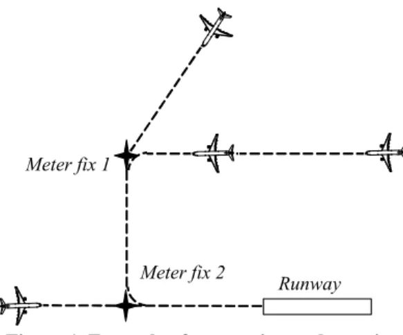
The main task of air traffic controllers managing arrival traffic is to sequence, merge and space aircraft for landing. An example of typical flight path for arriving aircraft at an airport is shown in Figure 1:
Runway Meter fix 1
Meter fix 2
Figure 1. Example of sequencing and merging operations for arriving aircraft at airport When one aircraft crosses the meter fixes, the following aircraft must be spaced at a prescribed minimum distance or time behind. Indeed, aircraft shall always be protected at least from wake turbulence generated by other aircraft. The minimum wake turbulence separation adopted by the civil aviation authorities depends upon the maximum takeoff weights of the aircraft involved ([1]).
The task of establishing properly spaced landing sequences is very demanding for air traffic controllers under heavy traffic conditions. As a consequence, automation tools named Arrival Manager (AMAN) often help air traffic controllers to build a sequence of aircraft in order to safely and expeditiously land them ([2]). Unfortunately, the airborne counterpart of the arrival manager which could help the flight crew to merge its aircraft towards a meter fix according to a sequence constraint is not yet available. Indeed, despite the fact that current aircraft’s Flight Management Systems (FMS) have the ability to navigate over predefined
paths, they are not capable of meeting a specified time-lag over meter fix relatively to another aircraft.
New concepts such as the delegation to the flight crew of some tasks presently performed by air traffic controllers have emerged during the last few years ([2]). More specifically, automatic merging and station keeping operations could relieve air traffic controllers of the need to provide time consuming radar vectoring instructions to the trailing aircraft once the flight crew has accepted the relative guidance clearance. Thus, the expected benefit of such new capabilities onboard aircraft is an increase of air traffic controller availability, which could result in increased air traffic efficiency and / or capacity. Enhancement of flight crew airborne traffic situational awareness with associated safety benefits is also expected.
As such a new capability onboard aircraft requires some surveillance and communication capabilities, and more specifically the knowledge of the leading aircraft position and velocity, the Automatic Dependent Surveillance-Broadcast
(ADS-B) is a potential key enabler to support these
surveillance requirements ([4]). Aircraft equipped with ADS-B capabilities broadcast their position, velocity and identification periodically (e.g. every second). Any neighboring aircraft capable of receiving those data will therefore be capable of tracking surrounding traffic.
Preliminary studies have mainly investigated the station keeping phase without taking into consideration the merging phase. This field is addressed for UAVs and military aircraft by means of linear feedback loop ([5]) or nonlinear feedback loop such as sliding mode control ([6]). However, research for civil aircraft where safety and passenger comfort are crucial issues is still in its initial stage. Indeed, [7] focuses on station keeping performed manually, whereas [8] develops a linear feedback loop (PID) limited to the control of longitudinal station keeping.
This paper investigates a linear and a new nonlinear design for both merging at a specified meter fix and station keeping. Eventually it compares both designs. This paper is the result of a joined effort between the French Air Navigation Study Center (CENA) which brings the operational concept and the French National College of Aviation (ENAC) which brings the competences in automatic control.
The paper is organized as follows: in the first section dealing with relative motion kinematics, inertial position dynamics, relative position dynamics and state space representation are introduced. Subsequent sections deal with the design of the linear
and the nonlinear feedback loops. Then, the statistical performance evaluation is performed and conclusions are raised.
Relative motion kinematics
Inertial position dynamics
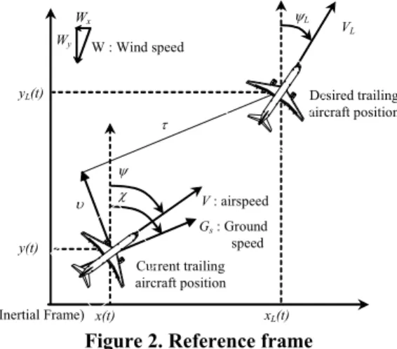
The considered reference frame is affixed to the current position of the trailing aircraft, as shown in Figure 2: x(t) Desired trailing aircraft position υ Current trailing aircraft position ψL y(t) yL(t) xL(t) VL V : airspeed ψ χ W : Wind speed Gs : Ground speed (Inertial Frame) Wx Wy τ
Figure 2. Reference frame
The along track distance, denoted by τ, is
aligned with the trailing aircraft ground speed vector,
whereas the cross track distance, denoted by υ, is the
distance from the current trailing aircraft position to the desired trailing aircraft position (i.e. the leading aircraft position a few minutes earlier) perpendicularly to its ground speed. The heading
angle of the trailing aircraft is denoted by ψ, its
airspeed by V. Subscript L is added for all variables related to the desired state vector.
Since wind is considered in this paper, the track
angle χ and the ground speed Gs are related to the
inertial velocity as follows:
( )
( )
⋅ = ⋅ = χ χ cos sin s s G y G x & & (1) Assuming that Earth is flat and non-rotating, it may be considered as an inertial frame. From Figure 2, the inertial position dynamics of the trailing aircraft are given by the following relations, whereψw denotes the direction from where the wind is
blowing and W its velocity:
( )
(
)
( )
(
)
− ⋅ + ⋅ = − ⋅ + ⋅ = π ψ ψ ψ π ψ w w W V y W V x cos cos sin sin & & (2) Those relations hold even if the motion of the aircraft in the vertical plane is considered as far as theflight path angle γ is small, which is a realistic assumption for commercial aircraft.
Referring to (1) and (2), the track angle χ and
the heading angle ψ are linked by the following
relations:
( )
( )
( )
( )
(
)
− ⋅ ⋅ ⋅ − + = ⋅ − ⋅⋅ − ⋅ = w s w w W V W V G W V W V ψ ψ ψ ψ ψ ψ χ cos 2 cos cos sin sin arctan 2 2 (3)Relative position dynamics
From Figure 2, the trailing aircraft desired position relatively to the current position of the trailing aircraft can be expressed in terms of the inertial positions as follows:
( )
(
( ) ( )
) ( )
(
( ) ( )
) ( )
( )
(
( ) ( )
) ( )
(
( ) ( )
) ( )
⋅ − − ⋅ − = ⋅ − + ⋅ − = χ χ υ χ χ τ sin cos cos sin t y t y t x t x t t y t y t x t x t L L L L (4)Taking into account the inertial position dynamics expressed in (2), and assuming the same wind for the leading and the trailing aircraft, the time derivative of (4) yields:
(
)
(
)
(
)
(
)
− ⋅ − − ⋅ + ⋅ − = − ⋅ − − ⋅ + ⋅ = χ ψ χ ψ τ χ υ χ ψ χ ψ υ χ τ sin sin cos cos V V V V L L L L & & & & (5)The time derivative χ& is obtained by
differentiating (3). As far as the track angle χ is a
function of
( )
V,ψ , its time derivative is a function of(
V,V&,ψ &,ψ)
. Note that it also depends on the windcharacteristics
(
W,W&,ψw,ψ&w)
that are generallyavailable on-board through the Air Data Computer (ADC).
State space representation
Denoting by u the control vector, by x1 and x2
the state vectors, and assuming that
(
W,W&,ψw,ψ&w)
and
(
VL,ψL)
are exogenous variable, equations (5) reduce to the following state space representation of the relative guidance kinematics:(
)
( )
= + ⋅ = u x x x u x x 2 2 1 2 1 , & & A B (6)where the state vectors x1 and x2 and the control vector u are defined by:
[ ]
[
]
[ ]
= = = T T T V V & & ψ ψ υ τ u x x 2 1 (7) and:(
)
(
)
(
)
( )
(
(
)
)
(
(
)
)
− ⋅ − − ⋅ − ⋅ − − ⋅ = − = χ ψ χ ψ χ ψ χ ψ χ χ sin sin cos cos 0 , , 0 , 2 2 2 2 V V V V B A L L L L x u x u x u x & & (8)It is worth noticing that vector B(x2) can also be
written according to the ground parameters:
( )
= ⋅ ⋅(
χ(
χ−χ−)
χ−)
L sL s L sL G G G B sin cos 2 x (9)This state space representation will be used for both the linear and nonlinear feedback loop designs, which are presented in the next paragraphs.
Linear feedback loop design
The design objective is to render the
equilibrium points
[ ]
T e 0 0 1 = x and[
]
T L L e=ψ V 2 x globally asymptotically stable.Since system (6) is nonlinear, a first alternative to design a feedback loop which stabilizes the system
around equilibrium points x1e and x2e consists in
linearizing the system. This is clearly a local approach, but it is the classical way to approach the stabilization problem for nonlinear systems ([9]).
Linearization of system (6) about x1e and x2e
results in the following linear system:
( )
(
)
(
)
= − ⋅ = − ⋅ ∂ ∂ = = u x x x x x x x x x x 2 2 2 2 2 2 2 1 ˆ 2 2 & & B e B e e (10) where:(
)
(
)
(
)
(
)
− − − − − − − = L L L L L L L L L L V V B χ ψ χ ψ χ ψ χ ψ sin cos cos sin ˆ (11)As far as the state vectors x1 and x2 are available
for feedback and the linearized system is completely state controllable, a pole placement technique can be applied in order to place the poles of the closed loop system at any desired location. To this end, the time derivative of the state vector x1 is derived once again:
u x x&1=Bˆ⋅&2=Bˆ⋅
& (12)
Now that the control vector u appears explicitly
from the time derivative of the output vector x1, the
dynamics of vector x1 is chosen so that it converges
towards the equilibrium point x1e. To that end, vector
x1 may obey to a second order linear differential
equation, where Λp and Λd stand for positive definite
feedback gain matrices (tuning parameters):
1 1
1 x x
x& =−Λd& −Λp
Gathering equations (3) and (4) leads to the expression of the control vector u:
(
1 1)
1 ˆ x x u=−B Λd +Λp − & (14) where:(
)
(
)
(
)
(
)
− − − − − − − = − L L L L L L L L L L V V B χ ψ χ ψ χ ψ χ ψ sin cos cos sin ˆ 1 (15)This resulting proportional and derivative (PD)
feedback loop is time varying since matrix ˆ−1
B is not
constant and evolves with heading and airspeed of the leading aircraft.
Using the first equation of (10), the feedback loop (14) is expressed in function of the available state vector x1 and x2:
(
)
(
2 2 1)
1 ˆ ˆ x x x u=−B Λd⋅B⋅ − e +Λp − (16)Coefficients of matrix Λd have the dimension of
sec−1 whereas coefficients of matrix Λp have the
dimension of sec−2.
Nonlinear feedback loop design
Since the nonlinear system (6) consists of two
cascaded systems with state vectors x1 and x2, and
taking into account the fact that the matrix A(x2,u) is
skew-symmetric, the recent vectorial backstepping design methodology ([10]) for construction of both feedback control law and associated Lyapunov functions can be applied to stabilize the system around the equilibrium points x1e and x2e.
In a first step, the virtual control B(x2) is chosen
in order to stabilize x1 around the equilibrium point
x1e:
( )
x2 =z2−Λ1x1B (17)
where Λ1 stands for a positive definite feedback
gain matrix (tuning parameter) and z2 is a new state
variable.
Then, a candidate Lyapunov function denoted by L1 is introduced for the x1-system, where k1 stands
for a positive parameter:
( )
1 1 1 1 1 2x x x k T L = (18)Taking into account (17) and the fact that the
matrix A(x2,u) is skew-symmetric, the time
derivative of (18) is:
( )
1 1 1 1 1 1 2 1 1 x x x z x T T k k L& =− Λ + (19)In a second step, the dynamics of z2 is obtained
by time differentiation of (17). Taking into account (6) leads to:
( )
( )
1 1 2 2 2 2 u z x x x x & & −Λ = ∂ ∂ = B dt dB (20)A candidate Lyapunov function for the whole model is:
(
1 2) ( )
1 1 2 2 2 2 1 ,z x z z x T L L = + (21)Taking into account (6) and (20), the time derivative of (21) is:
(
) ( )
= + Λ +∂∂( )
u x x x z x z x 2 2 1 1 2 1 1 2 1 2 , B LL& & T & (22) Finally, taking into account (19) leads to the following:
(
)
( )
∂ ∂ + Λ + + Λ − = u x x x x z x x z x 2 2 1 1 1 1 2 1 1 1 1 2 1 2 , B k k L T T & & (23) The matrix( )
2 2 x x ∂∂B has the following
expression:
( )
( ) ( )
( ) ( )
= ∂ ∂ 2 2 2 2 2 2 x x x x x x k h g f B (24) Where:( )
(
)
(
)
(
)
(
)
( )
(
)
(
)
(
)
(
)
( )
(
)
(
)
(
)
(
)
( )
(
)
(
)
(
)
(
)
− − − ∂∂ − − − = − − − ∂∂ − − − = − − − ∂∂ + − − = − − − ∂∂ + − = χ ψ χ ψ χψ χ χ ψ χ ψ ψχ χ ψ χ ψ χ ψ χ ψ χ χ ψ χ ψ ψχ χ ψ cos cos sin cos cos cos sin sin cos sin sin sin 2 2 2 2 V V V k V V V h V V V g V V V f L L L L L L L L x x x x (25)The partial derivatives ∂χ/∂ψ and ∂χ/∂V are
computed from (3).
Note that if wind is not considered (i.e. χ=ψ and
Gs=V) the above expressions reduce to:
( )
(
)
( )
( )
(
)
( )
= − − = − = − = 0 cos 1 sin 2 2 2 2 x x x x k V h g V f L L L L ψ ψ ψ ψ (26)The key point of the feedback loop design is
that matrix
( )
2 2 x x ∂( )
( )
−( )
( ) ( )
−( )
∆ = ∂ ∂ − 2 2 2 2 2 1 2 2 1 x x x x x x x f h g k B (27) Where:( )
(
)
(
)
− ∂∂ + ∂∂ − + − ∂∂ − = ∆ ψ ψ χ ψχ ψ ψ ψχ L L L L V V V V sin 1 cos 2 x (28)Finally, the control vector u is defined in order
to regulate the virtual output z2 to zero. This design
has been initiated in [11] and is based on the Young’s inequality, namely: 2 2 2 y x xy≤ + (29)
Taking into account (17) and the first equation of (6) into (23) leads to:
(
)
( )
(
)
( )
( )
∂ ∂ + Λ + Λ + + Λ − = u x x x z x u x I z x x z x 2 2 2 1 2 1 2 1 2 1 2 1 1 1 1 2 1 2 , , B B A k k L T T T & (30)Matrix I2 stands for identity matrix. For the
specific case studied in this paper, we will assume that matrix Λ1 is diagonal:
{
11 12}
1=diagλ ,λΛ (31)
As a consequence, the use of the Young’s inequality leads to:
( )
(
1 2 1 2)
1 1 1 1 2 2 2 2 2 1 2 1 ,u x x x z z x I zT k +ΛA ≤ TK + TK (32)where K1 and K2 are positive definite diagonal
matrices: + + = λ χ& λ χ& 11 1 12 1 1 0 0 k k K (33) + + = λ χ λ χ & & 12 1 11 1 2 0 0 k k K (34) Therefore (29) becomes:
(
)
( )
( )
∂ ∂ + Λ + + Λ − − ≤ u x x x z z x x z x 2 2 2 1 2 2 2 1 1 1 1 1 2 1 2 2 2 , B B K K k L T T & (35)In order to stabilize the (x1-z2) system, the
control vector u is chosen as follows, where Λ2
stands for a positive definite feedback gain matrix (tuning parameter):
( )
( )
+Λ +Λ ∂ ∂ − = − 2 1 2 2 2 1 2 2 2 z x x x u B K B (36)Thus the time derivative of the candidate Lyapunov function becomes:
(
)
1 2 2 2 1 1 1 1 2 1 2 2 ,z x x z z x − Λ Λ − − ≤ T K T k L& (37)The time derivative of the candidate Lyapunov
function L2 can be made negative definite by
choosing k1 and K1 such that:
0 2 1 1 1Λ − > K k (38)
This choice is always possible. Parameter k1 has
the dimension of sec−2, whereas matrices Λ1 and Λ2
have the dimension of sec−1.
Using equation (17), the feedback loop (36) is
expressed in function of the available state vector x1
and x2:
( )
( )
Λ +Λ + +Λ +Λ ∂ ∂ − = − 1 1 2 2 2 1 2 2 1 2 2 2 2 x x x x u K B K B (39)Statistical performance evaluation
Matching linear and nonlinear designs
In order to fairly compare the linear and the nonlinear designs, the matrices K2, Λ1, Λ2, Λp and Λdhave been chosen so that the backstepping feedback loop (39) and the proportional and derivative feedback loop (16) simplify to the same feedback
loop around the equilibrium point x2e. As a
consequence, the following identification has been made: Λ = Λ + Λ + Λ = Λ +Λ d p K K 1 2 2 1 2 2 2 2 (40)
In summary, the linear feedback loop is expressed as follows:
(
)
(
2 2 1)
1 ˆ ˆ x x x u=−B Λd⋅B⋅ − e +Λp − (41)Whereas the nonlinear feedback loop is:
( )
(
( )
)
1 2 1 2 2 x x x x u B ΛdB +Λp ∂ ∂ − = − (42)In order to comply with the time response of the airspeed and bank angle control channels for a wide body aircraft such as an Airbus A320 ([12]), the matrices Λp and Λd have been set as follows:
⋅ ⋅ = Λ ⋅ ⋅ = Λ − − − − − − 1 3 3 2 4 4 sec 10 16 0 0 10 16 sec 10 4 0 0 10 4 d p (43)
It is assumed in the following that two decoupled autopilot functions dealing with airspeed control and bank angle control are available onboard the trailing aircraft. These decoupled functions assume coordination between throttle, aileron and rudder, as in many modern jets. In order to comply with the time response of the airspeed and bank angle control channels, the controlled airspeed and the
controlled bank angle, denoted respectively by Vc
and φc, are set as follows during the simulations: u + = sec 50 0 0 0 V g V Vc c φ (44)
Relative guidance maneuver phases
The purpose of the relative guidance feedback loop is first to guide the trailing aircraft towards a merging meter fix and then to maintain station keeping behind the leading aircraft. As a consequence, the relative guidance maneuver is divided into two phases: the merging phase and the station keeping phase.
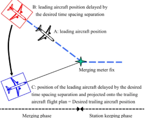
C: position of the leading aircraft delayed by the desired time spacing separation and projected onto the trailing aircraft flight plan = Desired trailing aircraft position B: leading aircraft position delayed by
the desired time spacing separation
A: leading aircraft position
Merging meter fix
Merging phase Station keeping phase
Figure 3. Leading aircraft targeted position mapped to the flight plan of the trailing aircraft
During the merging phase, and as shown in Figure 3, the current leading aircraft position (A) is delayed by the desired time spacing separation specified by air traffic control (B) and then projected onto the trailing aircraft flight plan (C). During this phase, the purpose of the relative guidance feedback loop is to track the delayed and projected leading aircraft position (position C).
As far as the delayed leading aircraft position has passed the merging meter fix, the projection onto the trailing aircraft flight plan is no more necessary.
Encounters data base
On the basis of the encounter geometry presented in Figure 3, many encounters have been generated by changing the angle between the two convergence legs, the length of the merging leg for the leading aircraft and the aircraft type, as shown in Figure 4: 20 NM Merging meter fix Sequencing measurement point Leading aircraft dl∈ {40 ;50} NM ds = dl+Vl×{0 ;180} sec Trailing aircraft ∆ψ ∈ {30 ;70 ;110 ;150} degrés Vl
Figure 4. Scenarios data base
The encounters of the data base have been generated as follows:
• The angle between the two convergence legs
varies between 30 and 150 degrees, with 40 degrees increment;
• The length of the merging leg for the leading
aircraft is set either at 40 NM or 50 NM;
• Six different aircraft types have been selected
from the Eurocontrol BADA database ([13]): ATR42/72, SAAB2000, A320, B767-300, A340, B747-400. Those types of aircraft are representative of the different type of propulsion, approach category and wake vortex category ([14]):
A/C type ATR 42/72 SAAB2000 A320 B767-300 A340 B747-400
Propulsion Turbo Turbo Jet Jet Jet Jet
Approach
Category B B C C D D
W. Vortex category
Med. Med. Med. Heavy Heavy Heavy
Table 1. Aircraft types
• At the beginning of the encounter, aircraft
start a descent at a flight level set between FL100 and FL260, as far as the selected flight level is flyable. They level off at FL100. The choice of the flight level sets the airspeed of the aircraft, which is compliant with the Eurocontrol BADA database ([13]) and varies between 266 kts and 492 kts;
• The initial position of the leading aircraft is
set at a distance from the merging fix equal to
dl+Vl×{0 ;180} seconds, where dl stands for the
the initial airspeed of the leading aircraft. As far as the objective for the relative guidance feedback loop is to place the following aircraft 90 seconds behind the leading aircraft, it shall delay or speed up the trailing aircraft by 90 seconds;
• A scenario is generated as far as the difference between the conventional airspeed of both aircraft is less than 30kts (airspeed compatibility) and as far as the expected distance to achieve the merging maneuver is greater than the actual distance between the initial position of the trailing aircraft and the point where the sequencing is measured.
Those considerations have lead to the generation of 1408 encounters in the data base.
Performance indicators
In order to assess the performances of both linear and nonlinear designs, three performance indicators have been computed:
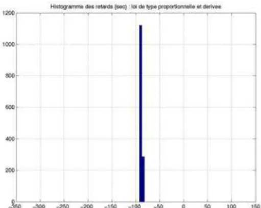
• The first indicator is the delay between the
leading and the trailing aircraft at the so-called sequencing measurement point. This point is placed 20 NM after the merging meter fix, where the station keeping phase is supposed to be achieved. This indicator is related with the quality of spacing. The histogram of this indicator for the encounter data base without any feedback loop is as follows:
Figure 5. Delay between the two aircraft at the sequencing measurement point without any
feedback loop
Without any feedback loop, the delay varies between -297 seconds and +71 seconds. The peaks of delays concentrate around values 0 and -180 seconds which are the values of delay chosen to calculate the initial position of the following aircraft. The variations around these values are due to the differences in speeds between the leader and the follower during the descent. The average of the delay
is -89 seconds, and the standard deviation is 97 seconds.
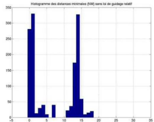
• The second indicator is the minimum distance
between the two aircraft and is related with the safety of the relative guidance maneuver. The histogram of this indicator for the encounter data base without any feedback loop is as follows:
Figure 6. Minimum distance between the two aircraft without any feedback loop
The minimum distance varies between 0 and
18 NM. The two peaks correspond to the
concentration of the delays around values 0 and -180 seconds. The average value of the minimal distance is 7.2 NM, and its standard deviation is 6.4 NM. There are 694 encounters for which the minimal distance is lower than 4.5 NM, and 624 encounters for which the minimal distance is lower than 2.5 NM.
• The third indicator relates to the dispersion of the difference between the conventional airspeed (CAS) of the leading and the trailing aircraft at the sequencing measurement point. This indicator is related to the operational acceptability of the relative guidance maneuver.
Figure 7. Difference between the conventional airspeed of the two aircraft at the sequencing measurement point without any feedback loop
The histogram of this indicator for the encounter data base without any feedback loop is depicted on Figure 7. Most of the encounters occur with aircraft without any differences in conventional airspeed.
Influence of linear and nonlinear feedback
loops
• The histogram of the delay between the
leading and the trailing aircraft at the sequencing measurement point is represented on the following figures:
Figure 8. Delay between the two aircraft at the sequencing measurement point with the linear
feedback loop
Figure 9. Delay between the two aircraft at the sequencing measurement point with the nonlinear
feedback loop
For the linear feedback loop, the delay varies between -91 seconds and -84 seconds. Its average is 88.6 seconds and the standard deviation is 1.6 seconds. For the nonlinear feedback loop, the delay varies between -91 seconds and -84 seconds. Its average is 88.8 seconds and the standard deviation is 2 seconds. As a consequence, the delay of 90 seconds between the two aircraft is achieved at the
sequencing measurement point for both linear and nonlinear feedback loop.
• The histogram of the minimum distance
between the two aircraft is represented on the following figures:
Figure 10. Minimum distance between the two aircraft with the linear feedback loop
Figure 11. Minimum distance between the two aircraft with the nonlinear feedback loop
The peak of both histograms is located in the set of minimum distance ranging between 6.5 and 7.5 NM. This set corresponds to a true airspeed of 288 kts (that is a conventional airspeed of 250 kts at FL100, which is the usual procedure for the jets which represent the majority of the encounters) multiplied by the desired delay of 90 seconds (which gives 7.2 NM).
For the linear feedback loop, the minimum distance ranges from 4 NM to 8.2 NM. Its average is 6.3 NM and the standard deviation is 1.1 NM. For the nonlinear feedback loop, the minimum distance ranges from 4 NM to 7.9 NM. Its average is 6.3 NM and the standard deviation is 1 NM.
The number of encounters for which the minimum distance is between 3.5 and 4.5 NM is the
same for the linear and the nonlinear design (114 encounters), but the nonlinear design places fewer encounters in the set between 7.5 NM and 8.5 NM.
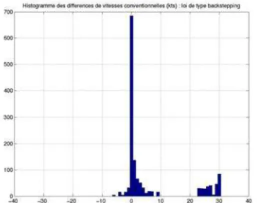
• The histogram of the difference between the
conventional airspeed (CAS) of the leading and the trailing aircraft at the sequencing measurement point is represented on the following figures:
Figure 12. Difference between the conventional airspeed of the two aircraft at the sequencing measurement point with the linear feedback loop
Figure 13. Difference between the conventional airspeed of the two aircraft at the sequencing measurement point with the nonlinear feedback
loop
For the linear feedback loop, there are 225 encounters for which the conventional airspeed (CAS) difference is +30 kts (i.e. the CAS of the following plane is 30 kts higher than the leading CAS at the sequencing measurement point), which indicates that the station keeping phase is not completely achieved (speed is not stabilized). For 355 encounters, the difference in speed is lower than 1.5 kts.
For the nonlinear feedback loop, there are only 84 encounters for which the conventional airspeed (CAS) difference is +30 kts. For 822 encounters, the
difference in speed is lower than 1.5 kts. This means that the time needed to achieve the station keeping phase is shorter with the nonlinear feedback loop, and consequently its operational acceptability would be greater.
Conclusion
This paper deals with the design of a new autopilot mode dedicated to both merging at a specified meter fix and station keeping behind a designated aircraft. This is achieved through a feedback loop which controls speed and bank angle.
The main contributions of this paper consist firstly in a new nonlinear design of the feedback control loop and secondly in a statistical performance evaluation between a linear design and the proposed nonlinear design, namely a proportional/derivative design and the proposed backstepping design.
The statistical performance evaluation is based on a data base of 1408 merging encounters which are operationally realistic. For both designs the delay between the leading and the trailing aircraft measured at a sequencing measurement point matches the desired delay between the two aircraft. In addition, both designs allow for safe merging and station keeping guidance. Nevertheless, the time needed to achieve the station keeping phase is shorter with the nonlinear feedback loop compared to the linear feedback loop. This promotes the nonlinear design. Indeed, a touch of complexity in the design process allows for better performances in the relative guidance feedback loop which would in turn allow for better operational acceptability.
The results have been obtained by maintaining the trailing aircraft on its flight plan during the simulations: this is adapted to correct delays between the leading and the trailing aircraft of a few minutes (90 seconds in this evaluation). For higher delays to be compensated, it may be valuable to reinforce the effect of the relative guidance feedback loop by stretching the trajectory of the trailing aircraft through the generation of a reference trajectory. This deserves further refinements and validations of the proposed approach.
References
[1] International Civil Aviation Organization, 2001, Air Traffic Services - Annex 11
[2] Kayton, Fried, 1997, Avionics navigation
systems, 2nd edition, John Wiley & Sons, New
[3] FAA-Eurocontrol cooperative R&D action plan 1, 2001, Principle of operations for the
use of ASAS, version 7.1
[4] Ivanescu, Hoffman, Zeghal, 2002, Impact of
ADS-B link characteristics on the performances of in-trail following aircraft,
Proceeding of AIAA GNC Conference, Monterey, USA
[5] Pachter, D’Azzo, Proud, 2001, Tight
formation flight control, Journal of Guidance,
Control, and Dynamics, Vol. 24, pp246-254 [6] Singh, Zhang, Chandler, Banda, 2003,
Decentralized nonlinear robust control of UAVs in close formation, International
Journal of Robust and Nonlinear Control, Vol. 13 pp1057-1078
[7] Agelii, Olausson, 2001, Flight Deck
Simulations of Station Keeping, Proceeding of
the 4th USA/Europe Air Traffic Management
Research and Development Seminar. Santa Fe, USA, Paper 17
[8] Vinken, Hoffman, Zeghal, 2000, Influence of
speed and altitude profile on the dynamics of in-trail following aircraft, Proceeding of
AIAA Guidance Navigation and Control Conference. Denver, USA, Paper No. 2000-4362
[9] Khalil, 2002, Nonlinear systems, 3rd Edition,
Prentice-Hall, New Jersey, Chap. 13, pp505-544
[10] Fossen, 2002, Marine Control Systems:
Guidance, Navigation and Control of Ships, Rigs and Underwater Vehicles
Marine Cybernetics, Trondheim, Chap 7, pp256-288
[11] Miquel, et al., 2004, Simplified Backstepping
Design for 3D Time Based Aircraft Relative Guidance, Proceeding of AIAA Guidance
Navigation and Control Conference, Providence, USA, Paper 2004-4993
[12] Favre, 1996, Fly-by-wire for commercial
aircraft: the Airbus experience. Advances in
Aircraft Flight Control, Taylor & Francis, London, Chap. 8, pp211-229
[13] Nuic, 2003, Aircraft Performance Summary
Tables for the Base of Aircraft Data (BADA) - Revision 3.4, EEC No. 06/02
[14] IAPA project, 2003, Implication on ACAS
Performances due to ASAS implementation: case study report, IAPA/WP04/029/D,
Eurocontrol ACAS Programme
Acknowledgements
The authors wish to thank Christelle Pianetti, and Philippe Louyot from the Centre d’Études de la Navigation Aérienne for their helpful inputs and comments.
Keywords
Airborne Separation Assistance System (ASAS), Sequencing and Merging Operations, Linear and Nonlinear Feedback Loop Design
Biographies
Thierry Miquel: he obtained his engineer degree from the ENAC school (French National College of Aviation) and did a master of science in signal processing in 1996. His obtained his PH.D in automatic control from the LAAS-CNRS (Laboratory of Analysis and Architecture of Systems - French National Center for Scientific Research) in 2004. He conducts research on ASAS algorithms at CENA.
Jean Marc Loscos: senior technical expert, head of the Airborne Surveillance, Collision Avoidance and Separation Department at CENA, representative of DSNA to ICAO and Eurocontrol groups dealing with ASAS (ICAO SCRS Panel, CASCADE Programme), responsible for DSNA in European Commission Projects on ASAS matters (G2G, ASSTAR).
Francis Casaux: he proposed in 1995 the ‘ASAS Concept’ to SICASP/WG2 (ICAO Panel). On behalf of EUROCONTROL he acted as CARE/ASAS manager and Point of Contact for Action Plan 1 (AP1) of the FAA/EUROCONTROL R&D Committee from September 1999 till December 2004. He is currently working for CENA (DGAC – France) in Toulouse.
Félix Mora-Camino: professor of Automatic Control and Avionics at ENAC school (French National College of Aviation). He is a senior Researcher at LAAS-CNRS (Laboratory of Analysis and Architecture of Systems- French National Center for Scientific Research).