HAL Id: hal-00938050
https://hal-enac.archives-ouvertes.fr/hal-00938050
Submitted on 27 May 2014
HAL is a multi-disciplinary open access
archive for the deposit and dissemination of sci-entific research documents, whether they are pub-lished or not. The documents may come from teaching and research institutions in France or abroad, or from public or private research centers.
L’archive ouverte pluridisciplinaire HAL, est destinée au dépôt et à la diffusion de documents scientifiques de niveau recherche, publiés ou non, émanant des établissements d’enseignement et de recherche français ou étrangers, des laboratoires publics ou privés.
commercial aircraft
Thierry Miquel, Felix Mora-Camino, Jules Ghislain Slama, Karim Achaibou
To cite this version:
Thierry Miquel, Felix Mora-Camino, Jules Ghislain Slama, Karim Achaibou. A nonlinear control approach for relative guidance of commercial aircraft. DINCON 2003, 2nd DLR/CTA Workshop on Data Analysis and Flight Control, Aug 2003, Sao Jose dos Campos, Brazil. �hal-00938050�
1 . SUMMARY
The delegation to the flight crew of tasks currently performed by the air traffic controllers provides a new perspective to significantly increase air traffic control capacity. Then, merging and station keeping operations have appeared to be of interest even if they rise new technical challenges. Indeed, these unusual maneuvers in the field of Civil Aviation seem difficult to be performed manually and since in this case they will result in an increase of the flight crew workload, new on-board automated functions should be developed. This paper investigates the design of an auto pilot mode dedicated to merging and station keeping maneuvers behind a leading aircraft. The proposed relative flight guidance law is based on a non linear sliding mode contr ol technique. Simulation results are displayed and discussed.
2. KEY WORDS
Relative Guidance, Flight Control Laws, Non Linear Control.
3. INTRODUCTION
The increase of air traffic urges the design of new devices to improve significantly air traffic control capacity [1] . So, to meet this challenge, new concepts such as “relative guidance” are presently of interest to contribute to the delegation of tasks to the crew [2]. The relative guidance function should provide an aircraft the ability to establish and to ma intain a given time or distance behind a designated aircraft (see figure 1). Nowadays no automatic control mode is available on-board civil aircraft to perform this task and few studies have been published in this field [3, 4].
This communication focuses on the design of a nonlinear controller which enables an aircraft to perform merging maneuvers and to maintain station keeping behind a designated aircraft. The inves tigated approach is based on the inversion of a simplified non linear model of the relative dynamics coupled with a sliding mode control technique. Preliminary evaluations are performed using simulation models of two wide body aircraft.
4. NOMENCLATURE
TK : along track distance XTK : cross track distance
ψ : heading angle of the trailing aircraft V : airspeed of the trailing aircraft
L : subscript added to all variables related to the leading aircraft
χ : track angle of the trailing aircraft Wx ,Wy : winds peed components
x,y : coordinates of the center of gravity of the trailing aircraft ρ : relative range
µ : relative bearing
τV : time constant of the controlled airspeed
X, y, u : state, output and control vectors s1, s2 : sliding mode surface variables
k1, k2, a11, a22, s1max,s2max : control parameters
5. RELATIVE FLIGHT DYNAMICS 5.1 ASSUMPTIONS AND DEFINITIONS
Some simplifying assumptions are made in this study: the maneuvers are performed at constant altitude over a considered locally flat and non rotating Earth. The wind speed vector is supposed to be the same for both aircraft. The Auto throttle controls the engines so that the
airspeed dynamics can be approximated by a first order linear model (time constant τV).
Heading is assumed to be controlled thr ough coordinated turns while roll and bank angle dynamics are neglected. Then, the variables characterizing the relative position of the trailing aircraft with respect to the leading aircraft are represented in the figure below:
x(t) Leading aircraft XTK TK Trailing aircraft ψL y(t) yL(t) xL(t) VL ground speed : airspeed χ ρ µ ψ W : Wind speed Vairspeed aairairspeedG (Inertial Frame)
Figure-2 Relative guidance parameters
5.2 STATE SPACE REPRESENTATION OF RELATIVE DYNAMICS
The range and the relative bearing of the two aircraft can be derived from the along track distance TK and the cross track distance XTK by:
2 2 XTK TK + = ρ and µ=ψ +arctg(XTK/TK) (1) while χ =arctg((Vsin(ψ)+Wx)/(Vcos(ψ)+Wy)) (2) These relations translate the variables manipulated by air traffic controllers and pilots (i.e. “merge 5 NM behind, 1 NM left”) into variables processed by the relative guidance device. The state vector retained here to describe the relative dynamics of the two aircraft is chosen as follows:
[
ρ, µ, V, ψ]
TX= (3) This leads to the following non linear affine state space representation of the relative guidance kinematics, where u denotes the control vector :
u X g X f X& = ( )+ ( ) (4) with u=
[
Vc, ϕ]
T (5) where − − − − − − − = 0 / / ) sin( ) sin( ) cos( ) cos( ) ( V L L L L V V V V V X f τ ρ µ ψ µ ψ µ ψ µ ψ and = V g X g V / 0 0 0 0 / 1 0 0 ) ( τ (6)The output vector, representative of the relative position of the aircraft, is chosen as :
[
ρ, µ]
Ty = (7) The control objective retained in this study is to lead the track variables to the respective desired values TKd and XTKd while the track angle of the trailing aircraft χ becomes equal to
the one of the leader. Through relations (1), this objective can be fully expressed with variables ρ, µ and χ. The resulting transient and permanent regimes should be compatible with the handling qualities of the aircraft and the required degree of comfort for a passenger aircraft.
5.3 THE RELATIVE GUIDANCE CONTROL LAW
Following non linear control theory [5], the relative degree of theses outputs is obtained through their derivation with respect to time until terms of the input vector appears. Here we get:
( ) ( )
X X u y =∆ +∆ ⋅ = µ 0 ρ && & & & & (8) with( )
(
)
(
)
(
)
(
)
(
)
(
)
(
)
(
)
(
)
(
)
(
)
− − − − − − − − −−−−−−−−−−−−−−− − − − − − − − + − = ∆ 2 0 / ] sin sin ) ( cos cos ) ( / sin [ sin sin ) ( / cos ρ µ ψ µ ψ ρ µ ψ µ ψ µ ρ τ µ ψ µ ψ µ ψ µ τ µ ψ V V X V V X V V V X V X L L L L V L L V & & & (9) and( )
(
)
(
)
(
)
(
)
− ⋅ − − − − ⋅ − − = ∆ µ ψ ρ ρτ µ ψ µ ψ τ µ ψ cos ) / ( ) /( sin sin / cos g g X V V (10)Note that in the above relations, the time rates of ψL and VL have been neglected. Here the
relative degrees of the outputs are both equal to two and the whole dynamics is covered by their dynamics. Then, there is no ground left for inner dynamics at this level of detail for the considered model of the relative flight dynamics. Moreover, as the rank of the matrix ∆(x) is in normal conditions (ρ >ρmin > 0) equal to 2 , this last relation can be inverted to get a non
linear control law such as:
( )
X y l( )
X u=∆ −1&&+ (11) with( )
(
)
(
)
(
)
(
)
− − − − − − − = ∆ − µ ψ ρ µ ψ µ ψ ρ τ µ ψ τ cos ) / ( sin ) / 1 ( sin cos 1 g g X V V (12) and l( )
X =−∆( )
X −1(
∆0( )
X)
(13)At this point, to fully determine the control law, a transient dynamics must be specified for the output vector y. In another work [6], the authors have evaluated the case in which the objective of the non linear inverse control law is to get linear decoupled output dynamics. This former approach has shown some strong limitations: high solicitation of the actuators leading to their saturation, generation of complex relative maneuvers and poor robustness with respect to modeling errors. Then the current study investigates the use of a modified sliding mode controller which leads the outputs to adopt progressively first order linear dynamics. Indeed, sliding mode control has been recognized to be a technique which can provide robustness in the control of non linear systems [7].
For the derivation of a sliding mode controller, let us select two switching surfaces as follows:
(
)
(
)
− + = − + = d d k s k s µ µ µ ρ ρ ρ 2 2 1 1 & & (14)where k1 and k2 are positive numbers, and ρd and µd are the desired range and relative bearing
derived from the desired along and cross track distances. Observe that their derivatives take
the form: + = µ ρ & & & & & & 2 1 2 1 k k y s s (16)
Then, a classical Lyapunov function [8] can be introduced: 2 2 2 1 2 1 2 1 s s W = + (17)
It is clear that if dW/dt is forced to remain negative, ρ and µ will be inclined to follow the above (relations (14)) first order sliding mode dynamics towards ρd and µd . For that, let us
choose a control law such that the derivatives of the switching surfaces satisfy:
( )
( )
− = − = 2 22 2 1 11 1 s sat a s s sat a s & & (18)where aii are positive parameters and the saturation functions are given by :
( )
> ∀ ≤ ∀ = max max max ) ( i i i i i i i i s s s s sgn s s s s sat (19)Then the relative guidance control law adopts the following expression:
( )
( )
( )
l( )
X k s sat a k s sat a X u + − ⋅ − − ⋅ − − ∆ = µ ρ & & 2 2 22 1 1 11 1 (20) 5.4 CASE STUDYDifferent scenarios have been des igned in order to evaluate the performances of the proposed control law. One of them is displayed here. This scenario considers an approach and includes the following features over a time period of 700 seconds for two wide body aircraft:
The leading aircraft starts at x0 = 0 NM, y0 = 0 NM, with an initial conventional airspeed
of 200kts and a heading of 90 degrees. The bank angle of the leading aircraft remains at zero, except between 220 sec and 320 sec, when the leader changes its heading by about 175 de grees (near a half circle) through setting at 20 the controlled bank angle . Furthermore, the controlled conventional airspeed of the leading aircraft is set to 160 kts for t > 600 sec, which
results in a deceleration. The trailing aircraft starts at x0 = -8 NM, y0 = +4 NM, with initial
conventional airspeed and heading of 200 kts and 90 degrees respectively. The requested separation for the trailing aircraft is 90 seconds behind the leading aircraft. The whole maneuver is supposed to take place within a wind of 20 kts blowing from North. During the maneuver, the inputs have been limited to ± 20° for ϕ with a maximum rate of ±5°/sec and to values between 140 kts and 250 kts for Vc with a maximum rate of ±1 kts/sec. The time
constant τV has been chosen equal to 40 seconds. The values of the parameters of the control
law have been taken as follows:
= = = = = = − − − sec / 05 . 0 sec, / 5 . 0 sec / 05 . 0 , sec 05 . 0 sec 1 . 0 , sec 01 . 0 max 2 max 1 2 1 1 1 22 1 11 NM s NM s NM k k a a (21)
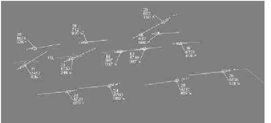
The trajectories of the leading and the trailing aircraft in the horizontal plane as well as the normal load factor are represented hereafter :
Figure-3 : Aircraft movement in the horizontal plane (axes in NM)
Figure-4 : Load factor(minus 1) versus time (in sec)
The evolutions with time of current delay and range between aircraft are shown in the following figures:
Leading aircraft: t=0 Trailing aircraft: t=0
Figure-5 : Current delay (in sec) between aircraft
Figure-6 : Current range (in NM) between aircraft
Finally, the figures below show the evolution w.r.t. time of the control variables:
Figure-7 : Controlled and actual airspeed (in kts) versus time (in sec)
Figure-8 : Controlled and actual bank angle (in degrees) versus time (in sec)
6. CONCLUSION
From the above preliminary results, it appears that non linear control theory provides theoretical grounds to perform the automation of relative guidance maneuvers. A possible control structure is displayed in figure 9. However ma ny difficulties remain. They are mainly related with the availability of reliable data exchange between aircraft and accurate relative navigation estimates, the development of new ATC officer’s and Pilot’s interfaces, the definition of new ground and on board procedures and the on board integration of this new flight guidance mode with the flight management system, the TCAS and the classical flight control and guidance modes.
Leading aircraft data {x,y,V,ψ} Desired relative position { Vc, ϕc} Trailing aircraft dynamics Leading aircraft dynamics Relative guidance controller Wind
Figure-9: A general relative guidance control structure
7. ACKNOWLEGMENTS
The authors wish to thank Mr Francis Casaux from CENA/EUROCONTROL-Brétigny and Professor Jean Lévine from Ecole Nationale Supérieure des Mines de Paris for helpful discussions during this research.
8. REFERENCES
[1] - European commission & Eurocontrol, 2002, “CARA/ASAS Activity 5 description of a
first package of GS/AS applications”, version 2.2, september.
[2] - Agelii M., Olavsson C., 2001,”Flight deck simulations of station keeping”, ATM 2001 R&D seminar, Santa Fe, paper no. 17.
[3] - Ivanescu D., Hoffman E., Zeghal K., 2002, “Impact of ADS-B link characteristics on
the performances of in -trail following aircraft”, AIAA Guidance, Navigation and Control
Conference, Monterey, USA, August.
[4 ]- Giulietti F., Pollini L., Innocenti M.,2000, “Au tonomous Formation Flight”, IEEE Control Systems Magazine, December.
[5] - Isidori A., 1989, “Nonlinear control systems”, Springer-Verlag.
[6] - Miquel T., Mora-Camino F.,2002, “Relative guidance of aircraft: analysis and
comparison of two control approaches”, World Aviation Congress, Paper No.
02WAC-55, November.
[7] - Mora -Camino F., Achaibou A.K., 1993, “Zero gravity atmospheric flight by robust nonlinear inverse dynamics”, AIAA J. of guidance, control and Dynamics, Vol.16,Num.3,pp604-607.
[8] – Slotine,J.J.,1984,”Sliding controller design for nonlinear systems”, International Journal of Control,vol.40,N°2,pp.421-434.