Science Arts & Métiers (SAM)
is an open access repository that collects the work of Arts et Métiers Institute of
Technology researchers and makes it freely available over the web where possible.
This is an author-deposited version published in:
https://sam.ensam.eu
Handle ID: .
http://hdl.handle.net/10985/7755
To cite this version :
Ludovic LAHOUSSE, Siriwan BORIPATKOSOL, Stéphane LELEU, Jean-Marie DAVID, Sébastien
DUCOURTIEUX, Thierry COOREVITS, Olivier GIBARU - LNE Activies in Nanometrology: flatness
reference calibration algorithm In: 8th euspen International Conference, Switzerland, 200805
-Proceedings of the 8th euspen International Conference - 2008
Any correspondence concerning this service should be sent to the repository
LNE Activies in Nanometrology: flatness reference calibration algorithm
L. Lahousse1, S. Boripatkosol2, S. Leleu2, J. David2, S. Ducourtieux1, T. Coorevits2,
O. Gibaru2
1LNE, Laboratoire National de Métrologie et d’Essais, France
2L2MA-Ecole Nationale Supérieure d’Arts et Métiers, France
1. Introduction
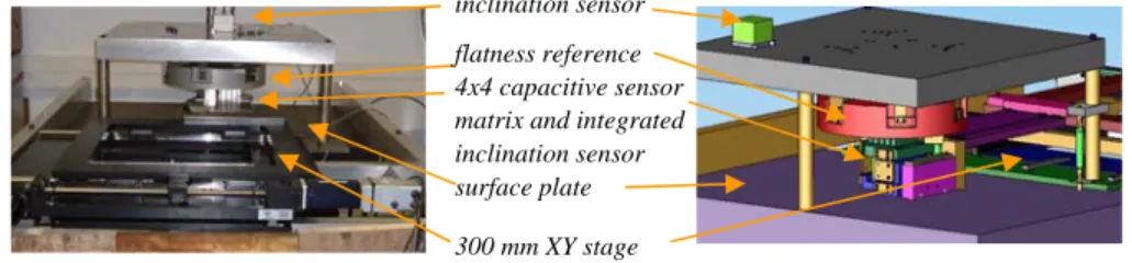
The Laboratoire National de Métrologie et d’Essais (LNE) has developed an innovative ultra precision coordinate measuring machine [LAH07] traceable to the national length standard to measure three-dimensional objects with nanometric uncertainties (figure 1). The measuring range is 300 mm x 300 mm x 50 µm. The objective in term of uncertainty is to reach 30 nm in X and Y directions for a displacement of 300 mm and about few nanometers for a vertical displacement of 50 µm. On this machine, we use
four capacitive sensors to measure the position along z direction. These sensors target the flat surface of cylinders (300 mm diameter) used as flatness references. To
measure the shape of these aluminum references with nanometric uncertainties,we
propose a measurement method based on a propagation process in which we introduce
an angular measurement to compensate the curvature error inherent in this method.
The measurement process uses the same sensor technology (capacitive sensor) we use on the machine. This paper presents the measurement method, its validation and the first results.
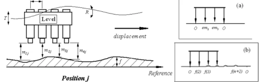
2. Propagation process with 4 capacitive sensors and an electronic level.
The measurement principle is based on a propagation process. We displace a matrix of sensors along the profile to measure [GAO96]. To introduce measurement redundancy, we use a matrix with 4 capacitive sensors. The distance d between each sensor is 20 mm (see figure 2). For each position j on the profile, we measure the
distance (m1j,…,m4j) which separates the capacitive sensor from the flatness reference.
The angular motion of the sensor matrix is measured thanks to an electronic level. The unknown parameters are the position of the electronic level origin compared to the origin of the capacitive sensors, the relative positions of the capacitive sensors and the
profile height called f. For each position j, we have to determinethe motion errors of
Figure 1: photograph of the machine
the matrix that we call Tj for translation errors and Rj for pitching errors.
Figure 2: straightness measurement using 4 capacitive sensors (left), convention used to locate the relative position of the sensor (a) the points of the profile (b)
As we use 4 sensors, only two parameters are necessary to characterize their relative positions. We call em2 and em3 the gap between the central sensor and the peripheral ones (figure 2a). The same way, we fix the profile extremities equal to zero (figure 2b). The general equations that link all the parameters are given in the reference [ELS05] and will not be presented here. Based on those equations, the system to be solved is:
For each position of the sensor matrix corresponds five lines in the system. The first four equations concern the distance measurement given by the capacitive sensor. The 5th equation concerns the angular measurement given by the electronic level. We use three methods to solve the system.
In the first method, we solve subsystems in which we favor capacitive sensor measurements. In this method, we proceed in two steps. First, the capacitive sensor information is used to start the resolution of the system. The resulting profile contains
⎥ ⎥ ⎥ ⎥ ⎥ ⎥ ⎥ ⎥ ⎥ ⎥ ⎥ ⎥ ⎥ ⎥ ⎥ ⎥ ⎥ ⎥ ⎥ ⎥ ⎥ ⎥ ⎥ ⎥ ⎦ ⎤ ⎢ ⎢ ⎢ ⎢ ⎢ ⎢ ⎢ ⎢ ⎢ ⎢ ⎢ ⎢ ⎢ ⎢ ⎢ ⎢ ⎢ ⎢ ⎢ ⎢ ⎢ ⎢ ⎢ ⎢ ⎣ ⎡ = ⎥ ⎥ ⎥ ⎥ ⎥ ⎥ ⎥ ⎥ ⎥ ⎥ ⎥ ⎥ ⎥ ⎥ ⎥ ⎥ ⎥ ⎥ ⎥ ⎥ ⎥ ⎥ ⎥ ⎥ ⎦ ⎤ ⎢ ⎢ ⎢ ⎢ ⎢ ⎢ ⎢ ⎢ ⎢ ⎢ ⎢ ⎢ ⎢ ⎢ ⎢ ⎢ ⎢ ⎢ ⎢ ⎢ ⎢ ⎢ ⎢ ⎢ ⎣ ⎡ ⎥ ⎥ ⎥ ⎥ ⎥ ⎥ ⎥ ⎥ ⎥ ⎥ ⎥ ⎥ ⎥ ⎥ ⎥ ⎥ ⎥ ⎥ ⎥ ⎥ ⎥ ⎥ ⎥ ⎦ ⎤ ⎢ ⎢ ⎢ ⎢ ⎢ ⎢ ⎢ ⎢ ⎢ ⎢ ⎢ ⎢ ⎢ ⎢ ⎢ ⎢ ⎢ ⎢ ⎢ ⎢ ⎢ ⎢ ⎢ ⎣ ⎡ − − − − − − + n n n n n n n n N m m m m N m m m m N m m m m const em em R T R T R T f f f d d d d d d d d d d d d 4 3 2 1 2 42 32 22 12 1 41 31 21 11 3 2 2 2 1 1 2 3 2 : : : : : : : 1 0 0 1 0 .. 0 0 0 0 0 .. 0 0 0 0 0 2 3 1 .. 0 0 0 0 0 .. 0 0 0 1 0 2 1 .. 0 0 0 0 1 .. 0 0 0 0 1 2 1 .. 0 0 0 0 0 .. 0 0 0 0 0 2 3 1 .. 0 0 0 0 0 .. 0 0 .. .. .. .. .. .. .. .. .. .. .. .. .. .. 1 0 0 0 0 .. 1 0 0 0 0 .. 0 0 0 0 0 0 0 .. 2 3 1 0 0 0 .. 0 0 0 1 0 0 0 .. 2 1 0 0 0 .. 0 0 0 0 1 0 0 .. 2 1 0 0 0 .. 1 0 0 0 0 0 0 .. 2 3 1 0 0 0 .. 0 1 1 0 0 0 0 .. 0 0 1 0 0 .. 0 0 0 0 0 0 0 .. 0 0 2 3 1 0 .. 0 0 0 1 0 0 0 .. 0 0 2 1 0 .. 1 0 0 0 1 0 0 .. 0 0 2 1 0 .. 0 1 0 0 0 0 0 .. 0 0 2 3 1 0 .. 0 0
a curvature error coming from the not perfect relative position of the sensors inside the matrix [GAO02]. The second step consists in using the level information to eliminate the curvature error without local modification of the profile.
In the second method, we use the information of the electronic level to calculate the rotation of the sensor matrix instead of the capacitive sensor measurement. In this method, we favor electronic level measurement
In the third method, we solve the whole system using the weighted least squares method that consist in dividing the system of equations by an estimation of each
measurement uncertainty. To solve the system, we minimise
(
)
2 N 1 i i i i ax b y
∑
= ⎟⎟⎠ ⎞ ⎜⎜ ⎝ ⎛ − + σ . As theweight of each measurement is inversely proportional to its uncertainty, the result is physically better. However, it is necessary to know the sensor measurement uncertainty and the level measurement uncertainty.
3. Experimental results
At the moment, to test the method, a dedicated bench was developed (figure 3).
Figure 3: developed bench
Two inclination sensors are integrated: one inside the capacitive sensor matrix and one above the flatness reference. The resolution of the inclination sensor is one micro-radian that is not sufficient to be comparable with the resolution of the capacitive sensors. Nevertheless, the repeatability of the inclination sensor is better than its resolution so it is possible to increase the resolution making the sensor oscillate. For that purpose, two piezoelectric actuators are introduced in the developed bench: one to rotate the sensor matrix and another one to make the reference oscillate. We suppose that the capacitive sensors and electronic level are not yet calibrated and that we do not
inclination sensor flatness reference 4x4 capacitive sensor matrix and integrated inclination sensor surface plate 300 mm XY stage
have a reliable estimation of their uncertainty. To compare the three solving methods, we introduce a parameter “L” which characterizes the ratio of the capacitive sensor measurement uncertainty with the electronic level measurement uncertainty
(
L
=
σ
senσ
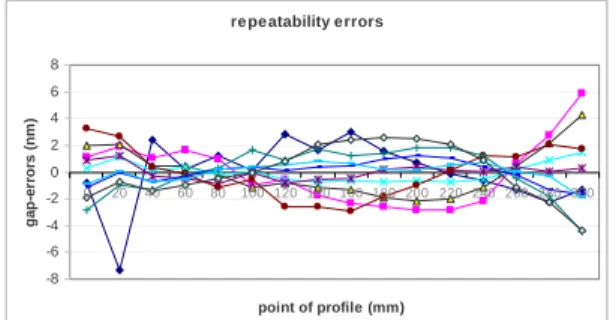
lev). The variation of this parameter corresponds to a change of theinformation weighting. We present on the figure 4, the deviation to the mean value of flatness reference straightness profiles obtained using the weighted least squares
method with “L” equal to one millimeter ⎜⎜⎝⎛ =xxµradnm ⎟⎟⎠⎞
lev sen
σ σ
. Each position corresponds to an average over one oscillation of the inclination sensor. The oscillation amplitude is 10 µrad. On this graph, we estimate the repeatability to +/- 4nm. This repeatability confirms the stability and the efficiency of the measurement.
repeatability errors -8 -6 -4 -2 0 2 4 6 8 0 20 40 60 80 100 120 140 160 180 200 220 240 260 280 300 point of profile (mm) ga p-e rr or s ( nm )
Figure 4: deviation to the mean value of straightness profiles obtained using the weighted least squares
On figure 5, we present the evolution of the straightness profile when the value of “L” changes. ‐2000 ‐1500 ‐1000 ‐500 0 500 1000 1500 2000 0 50 100 150 200 250 300 Pr o fi le er ro rs (n m ) point of profile (mm) straightness measurement‐ Variability depending on the method level preponderant Sensors preponderant -40 -30 -20 -10 0 10 20 30 40 0 20 40 60 80100 120 140 160 180 200 220 240 260 280 300 pro fi le err o rs (n m ) point of profile (mm) Straightness measurement-Gap-average L=0.1mm L=1mm L=3mm L=5mm L=7mm L=10mm L=15mm L=20mm L=30mm L=50mm L=100mm
Figure 5: Evolution of the profile for several choices of ”L”
We notice in Fig. 5 that the shape of the profile evolves between two extreme profiles corresponding to the two extreme methods. For high value of L (L=100 mm), the
profile converges to the one we obtain when we favor the level information (second method). When L is small (L=0.1 mm), the situation is reversed and the profile converges to the one we obtain when we favor the capacitive sensor information (first method).
The 60 nm deviation between the different methods is significant in regard of our objectives. This is due to the inconsistency of the capacitive sensor and electronic level information. The calibration of the two sensors will significantly decrease this inconsistency. The experimental evaluation of the sensor measurement uncertainty will allow fixing L and consequently to find the optimal weighting for the weighted least squares method.
4. Conclusion
The few nanometer repeatability of the profile measurement shows the efficiency of the method in which we increase the level resolution by averaging the measurement during level oscillations. The several methods used to solve the system show a deviation of 60 nm that corresponds to the inconsistency of the information coming from the electronic level and the capacitive sensors. When these sensors will be calibrated, we will use the weighted least squares method to improve the presented straightness measurement method.
References:
[ELS05] Elster C, Weingärtner I, Schulz M. “Coupled distance sensor systems for high-accuracy topography measurement: Accounting for scanning stage and systematic sensor errors.” Precision Eng.2006;30:32-38
[GAO96] Wei Gao, Satoshi Kiyono “ High accuracy profile measurement of a machined surface by the combined method” measurement vol.19, No. 1, pp.55-64, 1996
[LAH07] L. Lahousse, S. Leleu, J. David, O. Gibaru, S. Ducourtieux “Z calibration of
the LNE ultra precision coordinate measuring machine.” 7th euspen International
Conference2007.
[GAO02] Wei Gao, Jun Yokoyama, Hidetoshi Kojima, Satoshi Kiyono “Precision measurement of cylinder straightness using a scanning multi-probe system” Precision Eng.2002;26:279-288