A Partitioned Solution Algorithm for Concurrent Computation of Stress–Strain and Fluid Flow in Continuous Casting Process

HAL Id: hal-03193304

https://hal.archives-ouvertes.fr/hal-03193304

HAL is a multi-disciplinary open access

archive for the deposit and dissemination of sci-entific research documents, whether they are pub-lished or not. The documents may come from teaching and research institutions in France or abroad, or from public or private research centers.

L’archive ouverte pluridisciplinaire HAL, est destinée au dépôt et à la diffusion de documents scientifiques de niveau recherche, publiés ou non, émanant des établissements d’enseignement et de recherche français ou étrangers, des laboratoires publics ou privés.

A Partitioned Solution Algorithm for Concurrent

Computation of Stress–Strain and Fluid Flow in

Continuous Casting Process

Shaojie Zhang, Gildas Guillemot, Charles-André Gandin, Michel Bellet

To cite this version:

Shaojie Zhang, Gildas Guillemot, Charles-André Gandin, Michel Bellet. A Partitioned Solution Al-gorithm for Concurrent Computation of Stress–Strain and Fluid Flow in Continuous Casting Pro-cess. Metallurgical and Materials Transactions B, Springer Verlag, 2021, 52 (2), pp.978 - 995. �10.1007/s11663-021-02070-4�. �hal-03193304�

1

A partitioned solution algorithm for concurrent

1

computation of stress-strain and fluid flow in

2

continuous casting process

3

4

Shaojie Zhang, Gildas Guillemot, Charles-André Gandin and Michel Bellet*

5

6

MINES ParisTech, PSL Research University, CEMEF - Centre de Mise en Forme des Matériaux, CNRS UMR

7

7635, CS 10207, 1 rue Claude Daunesse, 06904 Sophia Antipolis cedex, France

8

9

Abstract: Control of macrosegregation phenomena and deformation related defects is a main issue in

10

steel continuous casting. Numerical simulation could help industrial engineers to master these defects.

11

However, as a first step, it is essential to achieve a concurrent computation of fluid flow in the bulk

12

liquid and stress-strain evolution in the already solidified regions. With this aim in view, a new specific

13

partitioned solver has been developed to model the liquid flow, essentially induced by the inlet jet

14

distributed by the submerged nozzle, as well as the thermal deformation of the solid shell. The solver

15

procedure allows simulating the transient regime, up to convergence to the steady-state regime. For this

16

purpose, the computational finite element mesh moves and grows continuously. Within this evolving

17

mesh, three different zones are defined: the solid shell as a pure Lagrangian zone, the liquid nozzle

18

region as a pure Eulerian zone, and an intermediate Eulerian-Lagrangian zone. Conservation equations

19

(energy, mass, and momentum) are solved in a general arbitrary Lagrangian-Eulerian framework, with

20

a level-set formulation to track the free surface evolution at the meniscus. The article is composed of

21

two parts. In the first part, the model is detailed with the resolution steps involved in the coupled

22

resolution approach. In the second part, a simple verification test case is firstly proposed, followed by a

23

more relevant and practical application to model an industrial pilot continuous casting process.

24

25

*Corresponding author. Tel.: +33 4 93 95 74 61, michel.bellet@mines-paristech.fr.

26

Email addresses: shaojie.zhang@mines-paristech.fr (S. Zhang), gildas.guillemot@mines-paristech.fr (G.

27

Guillemot), charles-andre.gandin@mines-paristech.fr (C.-A. Gandin), michel.bellet@mines-paristech.fr (M.

28

Bellet).

29

Metallurgical and Materials Transactions B 52 (2021) 978-995 doi.org/10.1007/s11663-021-02070-4

2

1 Introduction

30

Continuous casting (CC) is likely the most important steel casting process due to its productivity and

31

cost-efficiency. It is also a very sophisticated process as it involves numerous complex physical

32

phenomena. Supported by the rapid development of computational capacities during the last decades,

33

numerical modeling plays a more and more important role in the understanding and future developments

34

of the CC process for steel companies. CC modeling consists principally in at least four physical

35

phenomena: heat transfer, fluid flow, solid deformation, and solute transfer.

36

In the literature, most existing numerical models addressing CC can be classified into two categories. In

37

the first category, the focus is set on thermo-fluid analyses, ignoring the other two aspects. The approach

38

is essentially focused on what is named the primary cooling zone, that is the mold region where liquid

39

steel is delivered at high speed by a submerged entry nozzle. With these models, industrial issues related

40

to fluid flow can be investigated. Influence of process parameters such as the nozzle holes orientation,

41

casting speed and mold width, on fluid flow patterns was successfully predicted.[1, 2] _{Heat convection}

42

and other fluid flow related transport phenomena, for e.g. motion of argon gas bubbles and non-metallic

43

inclusions, can be modeled.[3, 4] _{Complex phenomena, such as interactions between fluid flow, slag}

44

infiltration and mold oscillations are also considered.[5] _{It is important to note that thermo-fluid}

45

simulation codes may give access to macrosegregation simulation by complementing the thermo-fluid

46

solver with an additional solver for transport of chemical species.[6, 7] _{By contrast, in the second category,}

47

numerical models focus on solid deformation. The main investigated industrial issues are still in primary

48

cooling: mold distortion and crack formation in solidified zones. But numerical codes for solid

49

mechanics also permit studying the deformation of the solid shell during secondary cooling, with defects

50

such as bulging between support rolls and associated crack formation.[8-10]

51

Following the presentation of these two categories - fluid flow and solid deformation - let us focus now

52

on the interest in coupling the two approaches in the context of CC modeling:

53

• First, the deformation of the solid shell in primary cooling may modify significantly the thermal

54

contact between the solid shell and the metallic mold, through the opening of a gas gap. This

55

gap appearance decreases drastically the heat exchange coefficient characterizing the heat flow

56

at product/mold interface. It is then easy to understand that an accurate simulation of the

57

solidification process in the mold region must take into account such changes in thermal

58

boundary conditions.

59

• Second, the prediction of the deformation and stress build-up in the solid shell in primary

60

cooling is generally addressed by use of solid structural codes (such as Abaqus for instance).

61

However, when proceeding this way, the influence of liquid convection loops in the mold region,

62

with localized critical zones such as those directly impacted by the hot nozzle jet, cannot be

63

taken into account. Hence, the prediction of cracking occurrence in the thin solid shell cannot

64

be accurate and reliable.

3

• Third, in secondary cooling, the interactions between the solid deformation and the

66

subsequently induced fluid flow in the mushy zone have been proven to have a dominant effect

67

on the formation of the central macrosegregation.[11] _{Therefore, an algorithm allowing the}

68

concurrent computation of stress-strain and fluid-flow is essential for a successful modeling of

69

such a phenomenon and furthermore to provide a more accurate model of solidification.

70

Regarding this coupling perspective, Thomas et al. have developed a strategy consisting in coupling

71

several independent simulation codes together: one code for fluid flow, a second one for shell

72

deformation.[12, 13] _{Zapulla et al. applied this approach to the simulation of the CC of stainless steel}

73

slabs,[12] _{while Koric et al. applied it to beam blanks CC.}[13] _{It should be noted that such a coupling}

74

approach relies on a sophisticated interface engineering, in order to ensure the exchange of information

75

between the different computational codes. This is all the more complex since this interface, namely the

76

surface at solidus temperature, continuously evolve during the simulation. This might be also a possible

77

source of robustness issues, or of efficiency loss in highly parallel computations. This is why the present

78

approach is somewhat different, aiming at achieving such coupled solid/fluid resolutions in a unique

79

computational code, and using a unique finite element mesh.

80

The coupled problem, as described above, can be seen as a general fluid-structure interaction (FSI) issue.

81

However, contrary to most FSI problems, the interaction considered here is between a very stiff structure

82

on one hand (the solid shell), and a low viscosity fluid on the other hand (the liquid metal). As pointed

83

out by Heil et al.,[14] _{the coupling effect between solid and fluid mechanics in a FSI problem can be}

84

characterized by a FSI index, defined as the ratio of the flow stress in the fluid and solid regions. It was

85

proven that for problems with a low FSI index, such as in the present problem for continuous casting, a

86

partitioned approach is more efficient than a monolithic approach. By partitioned approach, one should

87

understand a staggered resolution scheme in which separate fluid and solid problems are solved and

88

coupled, while a monolithic approach is for a unique resolution. The reason for the best performance of

89

the partitioned approach lies in the fact that the monolithic approach is affected by a loss of numerical

90

conditioning. Indeed, the spectrum of eigenvalues of the set of equations to be solved is too wide and

91

dramatically affects the convergence speed of iterative solvers. More detailed analysis can be found in

92

references [14] and [15].

93

Another characteristic feature of solid/liquid coupling in the context of solidification is the coexistence

94

of solid and liquid phases in mushy zones, where temperature is in between the liquidus and the solidus

95

(or eutectic) temperatures corresponding to the solidification interval. At the process scale, the interface

96

between the two phases cannot be explicitly modeled. Instead, the liquid and solid phases have to be

97

considered in a homogenized way within a mushy zone. In the literature, there are only a few numerical

98

models which are capable of coupling fluid flow and solid deformation. They were developed only in

99

recent years.[16-18] _{In those codes, fluid flow computation and stress-strain analysis are coupled and}

100

solved simultaneously within a single system of non-linear equations, expressing the momentum

101

conservation equations relative to the solid and liquid phases, together with global mass conservation.

4

They are not affected by numerical conditioning problems because they focus essentially on the mushy

103

zone deformation, without involving very stiff constitutive equations for solid metal. Such constitutive

104

equations derive from generalized non-Newtonian fluid behavior models. Some interesting results were

105

obtained with this approach. Koshikawa et al. studied the fluid flow and associated macrosegregation

106

induced by the lateral punching of an ingot deformed upon solidification, a specific solicitation aiming

107

at mimicking soft reduction in CC.[11] _{Fachinotti et al.}[16] _{and Rodrigues et al.}[18] _{directly addressed the}

108

simulation of soft reduction in CC. However, this approach is not retained in the present work for two

109

reasons: i) using such a behavior model for the solid, it is impossible to address the prediction of residual

110

stress in solid metal (as this requires elastic-(visco)plastic constitutive models such as the one described

111

in the work of Bellet and Thomas[19]_{), and ii) the computational cost is prohibitive. Actually, solving for}

112

the liquid and solid velocity fields in a unique set requires that 7 unknown values should be determined

113

at each node or cell of the computational grid: the 3 components of the solid velocity, the 3 components

114

of the liquid velocity plus a pressure unknown in case of a mixed velocity-pressure formulation. Hence,

115

7 unknowns instead of 4 (3 velocity components plus a pressure) results in a dramatic increase of the

116

computational time.

117

It is then clear that the partitioned approach is a good candidate to simulate FSI in CC. Similarly to the

118

previous work aiming at simulating ingot casting,[15] _{special care has to be put to consider the mushy}

119

zone in each of the two solvers. This is especially true in CC, where the solid phase in the mushy zone

120

is no more quasi-static, but moves at approximately the casting velocity. The global movement of the

121

solid phase requires in turn an Arbitrary Lagrangian Eulerian (ALE) formulation. In the present work,

122

a partitioned solution algorithm is then proposed for CC as an extension of the previous work done for

123

ingot casting application.[15] _{The numerical model principally consists of two resolution steps performed}

124

at each time increment on the same computational domain: the first one, labeled STEP I, is a

solid-125

oriented solution of the momentum and mass conservation equations, from which the stress-strain

126

analysis is carried out in the regions partially or completely solidified. The second one, labeled STEP

127

II, is a fluid-oriented solution of the momentum and mass conservation equations, giving access to the

128

velocity and pressure fields in the fluid-containing zones, i.e. regions with liquid, mushy zone and gas.

129

The volume averaging methodology and the Darcy’s law are used to model the interactions between

130

solid and liquid phases in the mushy zone. A characteristic feature of the present approach is that all

131

conservation equations are formulated in the framework of a level set method in order to track the

132

metal/gas interface. Another important point is that the partitioned algorithm is coupled with a

non-133

linear energy solver to calculate the temperature field. As this solver was initially developed by Saad et

134

al.[20] _{under a fixed solid phase hypothesis, it is also extended to consider the movement of the solid}

135

phase.

136

The paper is organized as follows. In Section 2 the algorithm is described with a special focus on the

137

above-mentioned extensions. In Section 3, a verification of the extended approach is demonstrated

138

through a simple case test. It is followed by a more relevant and practical application to an industrial

139

pilot continuous casting process.

5

141

2 Model description

142

2.1 Level set method: short reminder and notations

143

A representative elementary volume (REV) of the simulation domain 𝛺 is composed of two

sub-144

domains, as schematized in Fig. 1. A gas-subdomain 𝛺𝐺 _{is defined above a metal sub-domain 𝛺}𝑀_.

145

Three regions may be present in the metal sub-domain itself: a bulk liquid region, l, a fully solid region,

146

s, and a mushy zone made of a mixture of the two former regions, l + s. The level set method is used to

147

explicitly model the evolution of the metal/gas boundary during the continuous casting process, 𝛤. More

148

precisely, 𝛤 is represented by the zero-isovalue of the signed distance function 𝜑(𝒙, 𝑡), defined for any

149

point 𝒙 and time 𝑡 in 𝛺. The smoothed Heaviside function ℋ𝑀 _{is defined based on 𝜑(𝒙, 𝑡) as:}

150

where 𝜀 is the half-thickness of the transition zone around the metal/gas boundary.

151

Fig.1. Schematic illustration of the simulation domain, including metal and gas sub-domains. The metal/gas

boundary, 𝛤, is explicitly modeled through a diffusive level set transition zone, i.e. zone delimited by the two thick black dotted lines of thickness 2𝜀.

Respectively denoting 𝜓𝑀 _{and 𝜓}𝐺 _{the physical property 𝜓 related to the metal and gas sub-domains,}

152

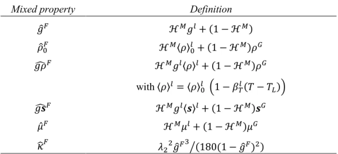
the mixed property 𝜓̂ is given by:

153

𝜓̂ = ℋ𝑀𝜓𝑀+ (1 − ℋ𝑀)𝜓𝐺 (2)

Thus, over the thickness [-𝜀, 𝜀] surrounding 𝛤, a smooth and continuous transition of properties is

154

defined. Note that the above-defined mixed property holds not only in the artificial transition zone

155

around the interface but also in the pure metal and gas sub-domains. Similarly, the mixed property 𝜓̂𝐹

156

associated with fluid, and being related to the liquid regions of the metal domain and the gas

sub-157

domain, can be defined by the following expression:

158

6

where 𝜓𝑙 _{refers to the intrinsic property associated with the liquid phase in the metal sub-domain.}

159

160

2.2 Moving mesh, and ALE formulation

161

The model of CC hereafter presented considers transient regimes. It aims at simulating non-steady states

162

of the process thus requiring a continuously growing computational domain. The mold that characterizes

163

the CC machine is of internal rectangular section. Its length defines the primary cooling region. The

164

mold itself is not directly modeled. Instead, initial and boundary conditions of the simulation domain 𝛺

165

are defined to account for its role in the solidification process. Initially, 𝛺 encompasses a metal

166

sub-domain 𝛺𝑀 _{in the primary cooling region (i.e., in the mold), plus the above located gas sub-domain}

167

𝛺𝐺_{. During the simulation, 𝛺}𝑀 _{grows in the casting direction at the velocity defined by the withdrawal}

168

speed, 𝒗_𝑐𝑐, progressively filling the whole primary cooling region, and then the secondary cooling zone

169

underneath the mold.

170

Fig.2. Schematics of the computational domain at (a) an early stage of the process when the metal is still fully

located in the mold region and (b) at a later stage when the metal occupies the full mold region and has entered the secondary cooling region. Typical dimensions are: width 0.5 to 1 m (for half of the product, as represented here), thickness 150 to 250 mm, height of the mold (primary cooling region) 600 to 800 mm, thickness of solid shell at mold exit 10 to 15 mm.

In this context, as explained hereafter, an evolving and constantly growing mesh is required. Fig. 2

171

illustrates the evolution of the computational domain 𝛺 at two different stages of the simulation,

172

respectively at an early stage (a) and at a later stage (b). At the top of the simulation domain, in 𝛺𝐺_as

173

well as in the neighborhood of the nozzle, a constant Eulerian zone is predefined where the mesh is

174

fixed. The dimensions of this Eulerian zone are defined at the beginning of the simulation and kept

175

unchanged all along the calculation. Its contour is drawn with thick green dotted lines in Fig. 2. In the

176

solidified shell, a convenient and accurate approach consists in having a mesh following the

177

displacement of the solid material. Indeed, the behavior of the solid material is elastic-viscoplastic, and

7

thus of memory type. As it will be seen below, the solution of incremental elasto-viscoplasticity is based

179

on total (or particle) time derivatives, which are extremely difficult to calculate accurately when using

180

a non-Lagrangian mesh (i.e. a mesh that would not evolve at the same speed as the material). For this

181

reason, a Lagrangian zone is defined, i.e. zone delimited by the contour using thick red dotted lines, as

182

shown in Fig. 2, corresponding to the fully solidified regions in the metal sub-domain. Unlike the

183

Eulerian zone, this Lagrangian zone keeps increasing during the simulation as it moves at material speed

184

in the solid shell (Lagrangian approach). Note that the bottom boundary of the simulation domain grows

185

at the casting speed with a vertical downward velocity, 𝒗_𝑐𝑐. The rest of the computational domain is

186

defined as an ALE zone, including the mushy zone and a part of the bulk liquid zone. The ALE zone is

187

delimited by the thick black dotted contour in Fig. 2. Like the Lagrangian zone, this zone keeps

188

increasing due to the imposed extraction speed of the machine which is prescribed along the bottom

189

surface. The mesh movement in this zone is rather arbitrary.

190

In the context of this work, the transition between the ALE zone (mobile mesh) and the Eulerian zone

191

(fixed mesh) is achieved through the use of a Heaviside function, ℋ𝐴𝐿𝐸_{. This Heaviside function is}

192

defined over the interface between the ALE and Eulerian zones, i.e. the coincident line of the thick

193

dotted green and black lines shown in Fig. 2. This Heaviside function, varying between 0 in the Eulerian

194

zone and 1 in the ALE zone, is smoothed over a certain thickness around the surface defined by ℋ𝐴𝐿𝐸 ₌

195

0.5, that is the interface between the two zones. This allows a smooth and progressive evolution of the

196

mesh dimensions that avoids excessive distortions. It should be mentioned that the location of this

197

interface is rather arbitrary: it depends on the definition of the Eulerian zone. Nonetheless, once this

198

interface is defined, it is kept unchanged over the whole simulation domain, and during the whole

199

simulation, as well as the associated Heaviside function defined above. The strategy to force a smooth

200

transition of the mesh evolution at the boundary between ALE and Lagrangian zones will be detailed in

201

the next section. As a summary, the simulation considers an evolving computational domain, with a

202

moving mesh composed of three regions:

203

• a fixed mesh in the gas and the nozzle neighborhood (Eulerian approach),

204

• a mesh moving at material speed in the solid shell (Lagrangian approach),

205

• a mesh having an arbitrary velocity in between.

206

The mesh velocity will be denoted 𝒗_𝑚𝑠ℎ in the sequel, the use of a moving mesh in turn inducing the

207

use of an ALE formulation to take into account 𝒗_𝑚𝑠ℎ in the discretization of conservation equations. In

208

ALE, the relationship between the partial time derivative of any physical quantity 𝜓 with respect to the

209

moving mesh, 𝜕_𝑚𝑠ℎ𝜓 𝜕𝑡⁄ (often named grid derivative), and the total time derivative 𝑑𝜓 𝑑𝑡⁄ , is resumed

210

in the following equation:

211

𝜕𝑚𝑠ℎ𝜓

𝜕𝑡 = 𝑑𝜓

𝑑𝑡 − (𝒗 − 𝒗𝑚𝑠ℎ) ∙ 𝛻𝜓 (4)

where 𝒗 represents the material velocity field. Note that in the case of a pure Eulerian framework,

212

𝒗𝑚𝑠ℎ≡ 0 and 𝜕𝑚𝑠ℎ𝜓 𝜕𝑡⁄ = 𝜕𝜓 𝜕𝑡⁄ . The relationship between the partial and total derivatives of 𝜓 is

213

8

then retrieved: 𝑑𝜓 𝑑𝑡⁄ = 𝜕𝜓 𝜕𝑡⁄ + 𝒗 ∙ 𝛻𝜓. In a pure Lagrangian framework, 𝒗𝑚𝑠ℎ≡ 𝒗, and Eq. (4)

214

simply expresses that 𝜕_𝑚𝑠ℎ𝜓 𝜕𝑡⁄ = 𝑑𝜓 𝑑𝑡⁄ . Finally, substituting the classical relationship 𝑑𝜓 𝑑𝑡⁄ =

215

𝜕𝜓 𝜕𝑡⁄ + 𝒗 ∙ 𝛻𝜓 into Eq. (4), an alternative relation is obtained:

216

𝜕𝑚𝑠ℎ𝜓

𝜕𝑡 = 𝜕𝜓

𝜕𝑡 + 𝒗𝑚𝑠ℎ∙ 𝛻𝜓 (5)

Hence, this allows for an easy adaptation and discretization of conservation equations in ALE. First, in

217

Lagrangian regions, it will be seen in Section 2.3 that only total derivatives are required. We have then

218

𝑑𝜓 𝑑𝑡⁄ ≡ 𝜕𝑚𝑠ℎ𝜓 𝜕𝑡⁄ , and the discretization is achieved by means of nodal finite differences:

219

(𝜓𝑛𝑡+Δ𝑡− 𝜓𝑛𝑡) Δ𝑡⁄ , where 𝑛 denotes a node of the moving mesh. Second, in all other regions (metal in

220

mushy or liquid state, gas) 𝒗_𝑚𝑠ℎ is different from the material velocity, and possibly null. Besides, it

221

will be seen in Sections 2.3 and 2.4 that the constitutive model is of no-memory type (viscoplastic or

222

Newtonian behavior), and that conservation equations require only partial time derivatives 𝜕𝜓 𝜕𝑡⁄ . They

223

will be replaced by 𝜕_𝑚𝑠ℎ𝜓 𝜕𝑡⁄ − 𝒗𝑚𝑠ℎ∙ 𝛻𝜓, according to Eq. (5). The time grid derivatives will be

224

discretized by means of nodal finite differences: (𝜓𝑛𝑡+Δ𝑡− 𝜓𝑛𝑡) Δ𝑡⁄ , where 𝑛 denotes a node of the

225

moving mesh.

226

227

2.3 STEP I: stress-strain analysis

228

As already mentioned above, the two resolution steps are successively performed at each time increment.

229

An important point is that they are operated on the same computational mesh covering the entire domain

230

𝛺. Hence, STEP I is not operated on the “solid” only; STEP II is not operated on the “liquid” only.

231

Instead, both STEP I and STEP II are solved on 𝛺.

232

The first resolution step is solid-oriented. This means that it essentially addresses the stress-strain

233

analysis in the solid regions and the mushy zone. The approach used was presented in detail in a previous

234

paper[15] _{and is briefly reminded here. The following momentum and mass conservation equations are}

235

solved for the velocity field 𝒗 and the pressure field 𝑝, using a finite element method:

236

{ ∇ ∙ 𝒔̂ − ∇𝑝 + 𝜌̂𝒈 = 0

∇ ∙ 𝒗 = ℋ𝑀(𝐻(𝑇𝐶− 𝑇)tr(𝜺̇𝑒𝑙) + tr(𝜺̇𝑡ℎ)) (6)

The tensor 𝒔̂ and the scalar 𝜌̂ are respectively the mixed stress deviator and the mixed density in domain

237

𝛺, as defined in Table 1. Vector 𝒈 is the constant gravity vector.

238

Mixed property Definition

𝒔̂ ℋ𝑀_𝒔𝑀_{+ (1 − ℋ}𝑀_)𝒔𝐺

𝜌̂ ℋ𝑀〈𝜌〉𝑀_{+ (1 − ℋ}𝑀_)𝜌𝐺

9

𝒔𝑀and 〈𝜌〉𝑀 _{are respectively the stress tensor and average density in 𝛺}𝑀_{. 𝒔}𝐺_{and 𝜌}𝐺_{are the stress tensor}

239

and density in 𝛺𝐺_{. The average metal density 〈𝜌〉}𝑀 _{is defined as 𝑔}𝑙_〈𝜌〉𝑙_{+ 𝑔}𝑠_〈𝜌〉𝑠 _{where 〈𝜌〉}𝑙 _{and 〈𝜌〉}𝑠

240

are respectively the intrinsic density of the liquid and solid phases with 𝑔𝑙 _{and 𝑔}s _{corresponding}

241

respectively to the local volume fractions of the liquid and solid phases.

242

𝐻(𝑇𝐶− 𝑇) is the standard Heaviside function, taken for the temperature difference (𝑇𝐶− 𝑇). It is

243

introduced as an indicator relative to the use of a thermo-elastic-viscoplastic (TEVP) constitutive model

244

for elements in the metal sub-domain with an average temperature lower than a certain critical transition

245

temperature 𝑇_𝐶, while a thermo-viscoplastic (TVP) model is used for elements in the metal sub-domain

246

with a temperature higher than 𝑇_𝐶.

247

Constitutive equations of the TEVP model, below 𝑇_𝐶, are described hereafter as given in reference [10]:

248

The strain rate tensor 𝜺̇ is split into an elastic part, 𝜺̇_𝑒𝑙, a viscoplastic part, 𝜺̇_𝑣𝑝, and a thermal part, 𝜺̇_𝑡ℎ

249

(Eq. (7)). The latter consists of the thermal expansion rate (Eq. (10)), with 𝜌 the density. Eq. (8) yields

250

the hypoelastic Hooke’s law where E represents the elastic tensor depending on the Young’s modulus

251

E, and the Poisson’s coefficient 𝜐. 𝝈̇ denotes the total time derivative of the stress tensor. Eq. (9) gives

252

the relation between the viscoplastic strain rate tensor and the stress deviator 𝒔. It is reminded here that

253

the stress deviator is defined as 𝒔 = 𝝈 − (1 3⁄ )tr(𝝈)𝑰 = 𝝈 + 𝑝𝑰, where 𝝈 is the Cauchy stress tensor, 𝑝

254

is the hydrostatic pressure, and 𝑰 is the identity tensor. Coefficient 𝐾 is the viscoplastic consistency, 𝜎𝑌

255

denotes the static yield stress below which no viscoplastic deformation occurs. The function [𝑥]+ is

256

equal to 0 when 𝑥 is negative and to the value 𝑥 otherwise. Coefficients 𝑚 and 𝑛 denote the strain-rate

257

sensitivity coefficient, and the strain hardening coefficient, respectively. Finally, the corresponding

258

relationship between the von Mises stress, 𝜎̅, the generalized plastic strain, 𝜀̅,and the generalized strain

259

rate, 𝜀̅̇, is given by:

260

𝜎̅ = 𝜎𝑌+ 𝐾(√3) 𝑚+1

𝜀̅̇𝑚_𝜀̅𝑛 ₍₁₁₎

Constitutive equations of the TVP model, over 𝑇_𝐶, are written as follows:

261

10

The strain rate tensor 𝜺̇ is split into a viscoplastic part, 𝜺̇_𝑣𝑝, and a thermal part, 𝜺̇_𝑡ℎ (Eq. (12)). Eq. (13)

262

is the classical constitutive law for a generalized non-Newtonian fluid. It relates the viscoplastic strain

263

rate 𝜺̇_𝑣𝑝 to the stress deviator 𝒔, in which the strain-rate sensitivity 𝑚 continuously increases with the

264

liquid fraction in the mushy zone. The Newtonian behavior, which is assumed to be the behavior law

265

for the liquid metal above its liquidus temperature, 𝑇_𝐿, as well as for the gas, is obtained for 𝑚 = 1. In

266

this case, the viscoplastic consistency 𝐾 is simply the dynamic viscosity of the fluid (liquid metal or

267

gas). Finally, the corresponding relationship between the von Mises stress 𝜎̅ and the generalized strain

268

rate 𝜀̅̇ is the following one:

269

𝜎̅ = 𝐾(√3)𝑚+1𝜀̅̇𝑚 (15)

In the present work, 𝑇𝐶 is taken exactly as the solidus temperature to model the TEVP behavior of steel

270

in a fully solid state; the TVP model is used for metal either in the mushy state or liquid state. At this

271

critical transition temperature, the continuity of the flow stress is obtained by taking 𝜎𝑌(𝑇𝐶) = 0 and

272

𝑛(𝑇𝐶) = 0.

273

Specific points of STEP I resolution

274

Two important characteristic features deserve attention:

275

• First, in order to prevent numerical instabilities due to the huge difference between solid consistency

276

and liquid or gas viscosities, the values of these latter properties are artificially augmented. The

277

liquid viscosity is typically set to 1 Pa · s, which is about 200 times the nominal value for liquid

278

steel for instance. The gas is considered as an incompressible Newtonian fluid in the gas sub-domain,

279

also with a viscosity typically set to 1 Pa · s. It is important to note that these simplifications have

280

no significant impact on the main focus of STEP I, which is the calculation of stress and strain in

281

already solidified regions during CC.

282

• A second important point in STEP I is the treatment of solidification shrinkage and liquid expansion.

283

Usually, when performing the solid-oriented resolution step alone, without STEP II, like in

284

reference [19], the thermal dilatation of both liquid and solid phases, are taken into consideration,

285

together with the solidification shrinkage. However, when adding STEP II to STEP I, another

286

strategy has been found more efficient. Keeping in mind that the focus of STEP I is the stress-strain

287

analysis in already solidified regions, only the solid thermal expansion is taken into account below

288

𝑇𝐿 (considering 〈𝜌〉𝑠 = 𝑓(𝑇) as an input). Especially, in the mushy zone, we are essentially

289

interested in the intrinsic velocity of the solid phase (i.e. the movement of the columnar dendritic

290

structure). Such a numerical approximation appears to be a simple but efficient way to achieve the

291

computation of a velocity field approaching the intrinsic velocity of the solid phase. In addition,

292

over 𝑇_𝐿, the material is considered incompressible: 〈𝜌〉𝑀_{≡ 〈𝜌〉}𝑠_(𝑇

𝐿). Hence, in Eq. (12), the thermal

293

11

part of the strain rate tensor, 𝜺̇_𝑡ℎ, is constantly null. The treatment of solidification shrinkage and

294

liquid expansion is done in STEP II and explained in the next Section.

295

Finally, a velocity-pressure resolution of the weak form of Eq. (6) is performed on 𝛺. The velocity and

296

pressure fields resulting from this first step are denoted (𝒗_𝐼, 𝑝𝐼).

297

298

2.4 STEP II: fluid flow computation

299

In this second fluid-oriented resolution step, the solution from the previous STEP I is taken as an entry.

300

The objective of this second step resolution is to calculate the fluid flow in liquid and mushy regions,

301

taking into account the motion of the solid phase, as deduced from STEP I. In order to consider liquid

302

flow through the permeable solid phase in the mushy zone, an effective two-phase approach is used with

303

a volume-averaged method.[21] _{Solidification is assumed to take place with a purely columnar structure.}

304

Interactions between solid and liquid phases in the mushy zone are modeled by the Darcy’s law with a

305

permeability coefficient 𝜅 approximated by the Carman-Kozeny relationship.[22] _{Although the liquid is}

306

considered as incompressible with a Newtonian behavior, a compressible formulation is used to deal

307

with solidification shrinkage in the mushy zone and thermal dilatation of the liquid phase. It is also

308

important to mention that in STEP II, contrary to STEP I, the nominal liquid viscosity is now used.

309

In a previous paper,[15] _{the conservation equations governing the fluid-oriented problem have been}

310

established in the context of a level set formulation applied to a static mesh. As mentioned in Section

311

2.2, its extension to the context of a mobile mesh is achieved by replacing the partial time derivatives

312

by the grid derivatives according to Eq. (5). The conservation equations for STEP II are now expressed

313

with the ALE formulation:

314

where the unknowns are the average fluid velocity, 𝒗 =ℋ𝑀𝑔𝑙_〈𝒗〉𝑙_{+(1 − ℋ}𝑀

)〈𝒗〉𝐺, and the pressure,

315

𝑝. Notations 𝜌̂0𝐹, 𝑔̂𝐹, 𝑔𝒔̂𝐹, 𝑔𝜌̂𝐹, 𝜇̂𝐹, 𝜅̂𝐹correspond respectively to the mixing properties of the fluid

316

density, the fluid fraction, the averaged fluid stress deviator, the averaged fluid density with temperature

317

dependence, the fluid viscosity and the fluid permeability. These variables are defined in Table 2.

12

Mixed property Definition

𝑔̂𝐹 _ℋ𝑀_𝑔𝑙_{+ (1 − ℋ}𝑀₎ 𝜌̂₀𝐹 _ℋ𝑀_〈𝜌〉 0 𝑙 _{+ (1 − ℋ}𝑀_)𝜌𝐺 𝑔𝜌̂𝐹 ℋ𝑀_𝑔𝑙_〈𝜌〉𝑙_{+ (1 − ℋ}𝑀_)𝜌𝐺 with 〈𝜌〉𝑙 = 〈𝜌〉0𝑙 (1 − 𝛽𝑇𝑙(𝑇 − 𝑇𝐿)) 𝑔𝒔̂𝐹 ℋ𝑀𝑔𝑙〈𝒔〉𝑙+ (1 − ℋ𝑀)𝒔𝐺 𝜇̂𝐹 ℋ𝑀_𝜇𝑙_{+ (1 − ℋ}𝑀_)𝜇𝐺

𝜅

Table 2. Mixed properties between the liquid regions of the metal sub-domain and the gas sub-domain in STEP II.

〈𝜌〉₀𝑙, 〈𝜌〉𝑙_{, 𝛽}

𝑇𝑙, 〈𝒔〉𝑙, 𝜇𝑙, 𝜆2 are respectively the intrinsic reference liquid density at 𝑇𝐿, the intrinsic liquid

319

density depending linearly from the temperature, the dilatation coefficient of the liquid, the intrinsic

320

liquid stress tensor, the liquid viscosity, and the secondary dendrite arm spacing. 𝜇𝐺 _{is the viscosity of}

321

the gas, assumed to be Newtonian and incompressible.

322

In the fully solid regions, there is actually no need to operate a STEP II resolution: all relevant

323

information (velocity field, updated values of the generalized viscoplastic deformation, deviatoric stress

324

tensor, and pressure) has been already calculated in the first solid-oriented resolution step. However, in

325

the present approach, STEP II is operated on the whole domain 𝛺, but with a Dirichlet condition applied

326

to the fully solid regions: for nodes with their nodal liquid fraction 𝑔𝑙 _{equal to zero, 𝒗}

𝐼𝐼 is imposed equal

327

to 𝒗_𝐼. Finally, Eq. (16) is solved with a stabilized SUPG-PSPG finite element method.[23] _{The velocity}

328

and pressure fields resulting from this second step are denoted (𝒗_𝐼𝐼, 𝑝𝐼𝐼).

329

330

2.5 Coupled thermal resolution

331

A non-linear energy solver is coupled with the above STEP I and STEP II to provide the temperature

332

field during the continuous casting process. The conventional energy conservation equation for

333

solidification problems is given in Eq. (17), averaged over the REV in the metal sub-domain:[21]

334

335

𝑔𝑠_〈𝑘〉𝑠_{+ 𝑔}𝑙_〈𝑘〉𝑙 _{with 〈ℎ〉}𝑙_{, 〈ℎ〉}𝑠_{, 〈𝑘〉}𝑙_{, 〈𝑘〉}𝑠_{, 〈𝒗〉}𝑙 _{and 〈𝒗〉}𝑠 _{corresponding respectively to the intrinsic}

336

specific enthalpy, the intrinsic heat conductivity and the intrinsic velocity relative to the liquid and solid

337

phases, respectively. Based on the relationship given in Eq. (5), the ALE formulation of Eq. (17) is given

338

by:

13

𝜕𝑚𝑠ℎ〈𝜌ℎ〉𝑀

𝜕𝑡 + 𝛻 ∙ 〈𝜌ℎ𝒗〉

𝑀_{− 𝒗}

𝑚𝑠ℎ∙ 𝛻〈𝜌ℎ〉𝑀− 𝛻 ∙ (〈𝑘〉𝑀𝛻𝑇) = 0 (18)

Developing the expressions of 〈𝜌ℎ𝒗〉𝑀 _{and 〈𝜌ℎ〉}𝑀_{, we obtain:}

340

Let’s first consider the following term, 𝛻 ∙ (𝑔𝑠_⟨𝜌⟩𝑠_⟨ℎ⟩𝑠_⟨𝒗⟩𝑠_{) − 𝒗}

𝑚𝑠ℎ∙ 𝛻(𝑔𝑠⟨𝜌⟩𝑠⟨ℎ⟩𝑠) in Eq. (19). This

341

term represents the energy transport related to the solid phase. Assuming that the volume change of the

342

solid, due to elasticity and thermal dilatation, has a negligible impact on heat transfer, the solid phase is

343

thus assumed here to be intrinsically incompressible, 𝛻 ∙ ⟨𝒗⟩𝑠_{= 0 . Therefore, the above term is}

344

simplified into the following form, (⟨𝒗⟩𝑠_{− 𝒗}

𝑚𝑠ℎ) ∙ 𝛻(𝑔𝑠⟨𝜌⟩𝑠⟨ℎ⟩𝑠). Note that in the bulk liquid this term

345

is zero. Besides, the fully solidified regions are considered as Lagrangian in the present ALE framework.

346

Therefore, in fully solidified regions, 𝒗_𝑚𝑠ℎ= ⟨𝒗⟩𝑠 _{and this term also reduces to zero.}

347

Finally, in the specific context of the present work, the mesh velocity 𝒗_𝑚𝑠ℎ in the mushy zone is

348

proposed with the following explicit form:

349

𝒗𝑚𝑠ℎ= 𝑔𝑙𝒗𝑐𝑐+ 𝑔𝑠𝒗𝐼 (20)

where 𝒗_𝐼 is the solution field from the previous solid-oriented resolution step and 𝒗_𝑐𝑐 the constant

350

casting velocity of the CC machine. We remind that 𝒗𝐼 is designed to approach the intrinsic solid

351

velocity ⟨𝒗⟩𝑠 _{in the previous solid-oriented resolution step. Besides, in continuous casting ⟨𝒗⟩}𝑠 _{in the}

352

mushy zone is nearly 𝒗𝑐𝑐 due to the continuity of the solid phase between the mushy zone and fully

353

solidified shell in contact with the molds. By consequence, the above-defined 𝒗𝑚𝑠ℎ keeps being a good

354

approximation of the intrinsic solid velocity ⟨𝒗⟩𝑠 _{in the mushy zone. Therefore, this first energy}

355

transport term related to the solid phase, (⟨𝒗⟩𝑠_{− 𝒗}

𝑚𝑠ℎ) ∙ 𝛻(𝑔𝑠⟨𝜌⟩𝑠⟨ℎ⟩𝑠), finally reduces to zero in the

356

whole metal sub-domain, including the bulk liquid, the mushy zone and the fully solidified regions, and

357

this term can be fully neglected from Eq. (19). In other words, the energy transport due to the motion of

358

the solid phase in the present model will be achieved through the mesh updating process within the ALE

359

framework. Finally, it is worth noting that the above-defined mesh velocity also holds in the fully

360

solidified regions, i.e. 𝑔𝑠_{= 1 and 𝒗}

𝑚𝑠ℎ recovers the material speed in the solid shell, 𝒗𝐼. A smooth

361

transition of mesh is thus ensured at the boundary of ALE and Lagrangian zones.

362

As stated above, the definition of the mesh velocity in the fully liquid zone is rather arbitrary and may

363

be different according to the specific configuration of each simulation. As explained in Section 2.2, a

364

pure Eulerian zone is usually defined with 𝒗𝑚𝑠ℎ = 0 in regions where metal remains in a liquid state,

365

for e.g. regions near the nozzle entry. More intuitive details of such a definition will be given later in

366

application to the CC process. Indeed, an optimized mesh velocity would be better to prevent mesh

367

distortions, such as the algorithm described in the work of Bellet and Fachinotti,[10] _{where the mesh}

368

14

velocity of a node in the liquid zone was defined roughly as the average velocity of its neighboring

369

nodes.

370

Considering now the second term 𝛻 ∙ (𝑔𝑙_⟨𝜌⟩𝑙_⟨ℎ⟩𝑙_⟨𝒗⟩𝑙_{) − 𝒗}

𝑚𝑠ℎ∙ 𝛻(𝑔𝑙⟨𝜌⟩𝑙⟨ℎ⟩𝑙) in Eq. (19), it represents

371

the energy transport related to the liquid phase. Assuming that the energy transfer due to the

372

solidification shrinkage and the thermal dilatation of the liquid phase is negligible, this term can be

373

approximated by 𝑔𝑙_⟨𝒗⟩𝑙_{∇(⟨𝜌⟩}𝑙_⟨ℎ⟩𝑙_{) − 𝒗}

𝑚𝑠ℎ∙ 𝛻(𝑔𝑙⟨𝜌⟩𝑙⟨ℎ⟩𝑙). We remind that 𝒗𝐼𝐼, the solution from the

374

previous fluid-oriented resolution step, represents the averaged liquid velocity, 𝑔𝑙_⟨𝒗⟩𝑙_{, in the liquid and}

375

mushy zones. In the meantime, it also tends to the solid velocity 𝒗_𝐼 when approaching the end of the

376

mushy zone due to the Dirichlet condition applied to the fully solidified regions. Therefore, the

377

following approximation is proposed for the above energy transport term related to the liquid phase:

378

𝑔𝑙_⟨𝒗⟩𝑙_{⋅ ∇(⟨𝜌⟩}𝑙_⟨ℎ⟩𝑙_{) − 𝒗}

𝑚𝑠ℎ∙ 𝛻(𝑔𝑙⟨𝜌⟩𝑙⟨ℎ⟩𝑙) = (𝒗𝐼𝐼− 𝒗𝑚𝑠ℎ) ∙ ∇(⟨𝜌⟩𝑙⟨ℎ⟩𝑙) (21)

Note that in the bulk liquid, 𝒗_𝐼𝐼 = 𝑔𝑙_⟨𝒗⟩𝑙_{, the right-hand side (RHS) term of Eq. (21) recovers exactly}

379

the left-hand-side (LHS) term of Eq. (21). In the fully solidified regions, the LHS term is zero as 𝑔𝑙_{= 0}

380

and RHS term is also zero as both 𝒗_𝐼𝐼 and 𝒗_𝑚𝑠ℎ equal to 𝒗_𝐼. Besides, in the mushy zone, Eq. (21)

381

remains a quite reasonable approximation, especially in regions with high liquid fraction where the

382

numerical solution 𝒗_𝐼𝐼 corresponds nearly to 𝑔𝑙_⟨𝒗⟩𝑙_{. Finally, assuming that contribution of the gradient}

383

of the liquid density is negligible in Eq. (21) and taking into consideration the enthalpy relationship

384

relative to the liquid phase, the above equation becomes:

385

(𝒗𝐼𝐼 − 𝒗𝑚𝑠ℎ) ∙ ∇(⟨𝜌⟩𝑙⟨ℎ⟩𝑙) = (𝒗𝐼𝐼− 𝒗𝑚𝑠ℎ) ∙ ⟨𝜌⟩𝑙⟨𝐶𝑝⟩ 𝑙

∇𝑇 (22)

where ⟨𝐶_𝑝⟩𝑙 is the intrinsic specific heat of the liquid phase defined by the liquid enthalpy ⟨ℎ⟩𝑙 ₌

386

⟨𝐶𝑝⟩ 𝑙

𝑇 + 𝐿𝑓 with constant latent heat of fusion 𝐿𝑓. Considering the above approximations made over

387

the energy transport term relative to both solid and liquid phases, the energy conservation equation in

388

the metal sub-domain for the CC process under the ALE framework is given by:

389

Finally, the energy conservation equation is developed under a level set formulation and is given by:

390

𝜕𝑚𝑠ℎ𝜌ℎ̂

𝜕𝑡 + (𝒗𝐼𝐼 − 𝒗𝑚𝑠ℎ) ∙ 𝜌𝐶̂𝑝

𝐹

∇𝑇 − ∇ ∙ (𝑘̂∇𝑇) = 0 (24)

with 𝜌ℎ̂ , 𝜌𝐶̂ , 𝑘̂ corresponding respectively to the mixing properties of the volumetric enthalpy, the 𝑝

391

volumetric heat capacity and the heat conductivity between the metal and gas sub-domains, defined in

392

Table 3.

15

Mixed property Definition

𝜌ℎ̂ ℋ𝑀〈𝜌ℎ〉𝑀_{+ (1 − ℋ}𝑀_)𝜌𝐺_ℎ𝐺 𝜌𝐶̂𝑝 𝐹 ℋ𝑀_⟨𝜌⟩𝑙_⟨𝐶 𝑝⟩ 𝑙 + (1 − ℋ𝑀_)𝜌𝐺_𝐶 𝑝𝐺 𝑘̂ ℋ𝑀_〈𝑘〉𝑀_{+ (1 − ℋ}𝑀_)𝑘𝐺

Table 3. Mixed properties between the metal and gas sub-domains in the coupled heat transfer step.

where ℎ𝐺_{, 𝐶}

𝑝𝐺 and 𝑘𝐺 are respectively the specific enthalpy, the specific heat and the heat conductivity

394

of the gas. It is worth noting that Eq. (24) holds for both continuous and ingot casting processes.

395

Especially, in a fully Eulerian framework where 𝒗𝑚𝑠ℎ= 0, Eq. (24) recovers the previous energy

396

conservation equation developed for ingot casting processes under a fixed-solid hypothesis.[15]

397

398

2.6 Algorithm scheme

399

The algorithm scheme of the present partitioned solution algorithm for continuous casting is presented,

400

considering that the two resolutions, STEP I and STEP II, and the coupled thermal resolution are

401

performed once at each time increment Δ𝑡. The incremental resolution scheme is divided into 7 modules,

402

as detailed hereunder in Fig.3:

403

16

• Coupled thermal solution. The energy conservation equation is solved, giving access to the

404

temperature distribution in the metal and gas sub-domains, and to the liquid metal fraction.

405

• STEP I, solid-oriented solution. The first folder of the mass and momentum conservation

406

equations focuses on the stress-strain analysis in the already solidified regions, with an

407

augmented liquid viscosity and a continuity of solid density in the mushy and liquid regions. It

408

provides velocity and pressure fields on the whole domain: (𝒗_𝐼, 𝑝𝐼). However, only 𝒗𝐼 at nodes

409

belonging to fully solid elements and in the mushy zone will be used in the follow-up of the

410

resolution scheme. The stress tensor 𝝈, and the associated generalized plastic strain 𝜀̅ and strain

411

rate 𝜀̅̇, are also deduced from this step.

412

• STEP II fluid-oriented solution. The second folder of the mass and momentum conservation

413

equations consists of the fluid flow computation in the liquid and mushy regions, with a real

414

liquid viscosity and including solidification shrinkage. It provides velocity and pressure fields

415

on the whole domain: (𝒗_𝐼𝐼, 𝑝𝐼𝐼). Note that at nodes belonging to fully solid elements, 𝒗𝐼𝐼 is

416

imposed equal to 𝒗_𝐼.

417

• Mesh updating. The position of each mesh node is updated following an explicit scheme with

418

the mesh velocity, 𝒗_𝑚𝑠ℎ:

419

𝒙𝑛𝑒𝑤 = 𝒙𝑜𝑙𝑑+ 𝛥𝑡𝒗𝑚𝑠ℎ (25)

It should be reminded that the energy transportation relative to the solid phase in the solid and

420

mushy zones, is achieved through this mesh updating process under the present ALE framework.

421

• Metal/gas interface tracking. The updating of the level set function permits interface tracking.

422

It is achieved by the convection-reinitialization scheme.[24] _{The advection velocity field 𝒗 is}

423

equal to the fluid velocity 𝒗_𝐼𝐼 deduced from STEP II.

424

• Mixing of material properties according to the value of the updated level set function.

425

• Possible adaptive remeshing guided either by error estimation for different solution fields, as

426

proposed by Coupez,[25] _{or more simply formulated based on signed level set distance function.}

427

428

3 Simulation results

429

3.1 Verification test case

430

The objective of the test case detailed hereafter is to check the correct implementation and the

431

performance of the above-proposed partitioned solution algorithm, including the new features

432

introduced in the thermal solver, i.e. introduction of the solid movement, the energy transport relative

433

to the solid phase and the mesh velocity. For this specific purpose, a simple solidification process

434

configuration is studied, in which the gas sub-domain is neglected, as the new developments mainly

17

affect the metal sub-domain. Besides, the solid-oriented step is oversimplified: no effective stress-strain

436

analysis is performed. Only the velocity of the solid phase is imposed, its value being equal to the

437

constant casting speed of the machine.

438

439

3.1.1 Model description

440

The test case consists of the solidification of two identical 3D parallelepipedic ingots, under the same

441

heat boundary condition. The first ingot is fixed and serves as the reference simulation. Its solidification

442

is simulated using the previous algorithm developed for casting process.[15] _{The second ingot is entirely}

443

submitted to a constant downward movement and is simulated with the algorithm presented above. For

444

simplicity, only the configuration of the moving ingot simulation is presented here as shown in Fig.4.

445

𝑣𝑐𝑠𝑡 denotes the value of the downward moving velocity. The initial mesh is isotropic, defined with a

446

uniform mesh size of 1 mm. A constant mesh velocity 𝒗_𝑚𝑠ℎ is defined over the whole ingot, oriented

447

downward and aligned on the vertical z-direction, with a module equal to 𝑣_𝑐𝑠𝑡. As the mesh velocity is

448

identical for all mesh nodes, the mesh will keep unchanged all along the simulation. Note that for the

449

reference simulation, the geometry and its discretization are the same as for the moving ingot at initial

450

state. Nonetheless, the value of mesh velocity is null and by consequence, a fixed mesh will be used for

451

the whole simulation.

452

Fig.4. Geometry of test case simulation of the moving ingot under solidification

Indeed, this moving simulation could be seen as a representation of a fixed slice of the metal product

453

for the CC process. Due to the symmetry of the system, only half of the slice is modeled. The six faces

454

of the ingot are numbered in order to clearly describe the boundary conditions. Note that the left face,

455

as well as the backward and forward faces, are defined as symmetry planes. In the following, the

456

associated thermal and mechanical boundary conditions, for the moving ingot simulation, are

457

summarized in Table 4.

18

Face position in Fig.4

Thermal boundary conditions

Mechanical boundary conditions

Fixed ingot (reference) Moving ingot ❶ Left Adiabatic Sliding (𝒗 ∙ 𝒆𝑥= 𝟎) Sliding (𝒗 ∙ 𝒆𝑥 = 0)

❷ Down Flux by convection Sticking (𝒗 = 𝟎) Constant velocity (𝒗 = −𝑣_𝑐𝑠𝑡𝒆𝑧)

❸ Right Flux by convection Sticking (𝒗 = 𝟎) Constant velocity (𝒗 = −𝑣𝑐𝑠𝑡𝒆𝑧)

❹ Backward Adiabatic Sliding (𝒗 ∙ 𝒆𝑦= 0) Sliding (𝒗 ∙ 𝒆𝑦= 0)

❺ Forward Adiabatic Sliding (𝒗 ∙ 𝒆𝑦= 0) Sliding (𝒗 ∙ 𝒆𝑦= 0)

❻ Top Adiabatic Sticking (𝒗 = 𝟎) Constant velocity (𝒗 = −𝑣𝑐𝑠𝑡𝒆𝑧)

Table 4. Thermal and mechanical boundary conditions for the solidification test case

Heat is extracted from the metal through the right face and the bottom face using a convection-type

459

expression for heat flux density, 𝑞_𝑇 = ℎ𝑇(𝑇 − 𝑇𝑒𝑥𝑡), where the heat transfer coefficient ℎ𝑇 and the

460

external temperature 𝑇_𝑒𝑥𝑡 are constant. The metal is supposed to slide along the surrounding faces

461

except at the top, bottom and left faces, on which a constant velocity 𝑣_𝑐𝑠𝑡 is imposed in the z-direction

462

𝒆𝑧. It should be reminded that the above-defined mechanical boundary condition is only applied in STEP

463

II, as STEP I is over-simplified with solution 𝒗_𝐼 predefined, equal to −𝑣_𝑐𝑠𝑡𝒆𝑧, over the whole metal

464

domain. Finally, note that for the reference simulation with fixed ingot, the energy boundary condition

465

is the same as the above-detailed moving ingot simulation. For the mechanical boundary condition,

466

sticking boundary condition is imposed on the top, bottom and left faces and all other faces are supposed

467

to be purely sliding.

468

The initial temperature of the metal 𝑇_𝑖𝑛𝑖 is chosen as the liquidus temperature 𝑇_𝐿. Densities of the liquid

469

and solid phases, ⟨𝜌⟩𝑙 _{and ⟨𝜌⟩}𝑠_{, are taken as constant and equal to the value at 𝑇}

𝐿, 𝜌𝐿. Hence,

470

solidification shrinkage is neglected and metal is assumed incompressible. Despite this assumption, in

471

the momentum conservation equation relative to the liquid phase, the thermal convection in the liquid

472

phase is taken into consideration by using the Boussinesq expression for the intrinsic liquid density:

473

⟨𝜌⟩𝑙 _{= 𝜌}

𝐿(1 − 𝛽𝑙(𝑇 − 𝑇𝐿)) , where 𝜌𝐿 denotes the density of the liquid phase at the liquidus

474

temperature and 𝛽𝑙 _{the thermal dilatation coefficient of the liquid phase. In the specific context of this}

475

verification test case, the solidification path is considered in an oversimplified form, assuming that the

476

volume fraction of the solid phase evolves linearly with temperature in the solidification interval.

477

The values of process, numerical, and material parameters used in this first test are summarized in Table

478

5. Regarding material properties, they should be seen as representative of a carbon steel. As such, they

479

are issued from different references and are simplified. For example, in this test, the thermal conductivity

480

is assumed to be constant and equal for both the liquid and the solid phase. The latent heat of fusion is

19

also taken as constant. Nonetheless, two constant but different values are taken for the specific heat

482

capacity relative to liquid and solid phases.

483

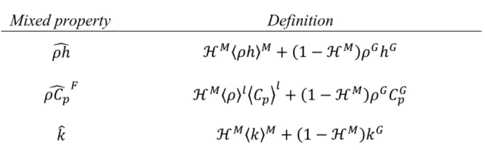
Material parameters Symbol Value Unit

Solidus temperature 𝑇𝑆 1499 °C

Liquidus temperature 𝑇𝐿 1552 °C

Densities 𝜌𝐿, ⟨𝜌⟩𝑙, ⟨𝜌⟩𝑠 7060 kg · m−3

Thermal dilatation coefficient of liquid 𝛽𝑙 2.95 × 10−4 °C−1

Secondary dendritic arm spacing 𝜆2 5 × 10−4 m

Liquid viscosity 𝜇𝑙 4.2 × 10−3 Pa · s

Solid specific heat ⟨𝐶𝑝⟩

𝑠

400 J · kg−1· °C−1

Liquid specific heat ⟨𝐶𝑝⟩

𝑙

800 J · kg−1· °C−1 Thermal conductivity for solid and liquid phases 〈𝑘〉𝑙_{, 〈𝑘〉}𝑠 _{30 W · m}−1_{· °C}−1

Latent heat of fusion 𝐿𝑓 3.09 × 105 J · kg−1

Process and numerical parameters

Initial temperature 𝑇𝑖𝑛𝑖 1552 °C

External temperature 𝑇𝑒𝑥𝑡 25 °C

Heat transfer coefficient ℎ𝑇 1000 W · m−2· °C−1

Downward moving velocity 𝑣𝑐𝑠𝑡 0.016167 m · s−1

Time step ∆𝑡 0.1 s

Table 5. Values of material and numerical parameters used for the verification test case.

484

3.1.2 Results

485

Fig. 5 illustrates the progress of the ingot solidification at time 𝑡 = 40 s. In Fig. 5a, results on the front

486

symmetry plane are shown, comparing the reference static ingot simulation (left half part of the figure)

487

and the moving ingot simulation (right half part). More precisely, the left part of Fig. 5a illustrates the

488

temperature field, 𝑇, and the fluid flow, 𝒗_𝐼𝐼, in the reference static ingot simulation. Note that the

489

velocity field can also be considered as 𝒗_𝐼𝐼− 𝒗𝑚𝑠ℎ, as 𝒗𝑚𝑠ℎ is indeed null in such a pure Eulerian

490

framework simulation. The right part of Fig. 5a describes the temperature field, 𝑇, and the relative fluid

491

flow, 𝒗_𝐼𝐼− 𝒗𝑚𝑠ℎ, for the moving ingot simulation in which 𝒗𝑚𝑠ℎ= −𝑣𝑐𝑠𝑡𝒆𝑧 is imposed to the whole

492

computational mesh. It should be mentioned that the spatial positions of the two ingots are indeed

493

different, i.e. with a relative vertical distance difference. The two simulation results (separated by the

494

dotted black symmetric line) are put side by side in order to facilitate comparison.

495

It can be seen that, by eliminating the mesh velocity 𝒗_𝑚𝑠ℎ, the same velocity field is found, which

496

corresponds in both simulations to the velocity induced by the thermal convection in the liquid phase.

497

Moreover, an identical temperature field is recovered in the moving ingot simulation compared to the

498

reference static ingot simulation. The liquidus and solidus isotherms, highlighted with white lines, are