HAL Id: hal-01509485
https://hal-mines-paristech.archives-ouvertes.fr/hal-01509485
Submitted on 16 May 2018
HAL is a multi-disciplinary open access
archive for the deposit and dissemination of
sci-entific research documents, whether they are
pub-lished or not. The documents may come from
teaching and research institutions in France or
abroad, or from public or private research centers.
L’archive ouverte pluridisciplinaire HAL, est
destinée au dépôt et à la diffusion de documents
scientifiques de niveau recherche, publiés ou non,
émanant des établissements d’enseignement et de
recherche français ou étrangers, des laboratoires
publics ou privés.
Statistical analysis of dislocations and dislocation
boundaries from EBSD data
Charbel Moussa, Marc Bernacki, Rémy Besnard, Nathalie Bozzolo
To cite this version:
Charbel Moussa, Marc Bernacki, Rémy Besnard, Nathalie Bozzolo. Statistical analysis of
disloca-tions and dislocation boundaries from EBSD data. Ultramicroscopy, Elsevier, 2017, 179, pp.63-72.
�10.1016/j.ultramic.2017.04.005�. �hal-01509485�
1
Statistical analysis of dislocations and dislocation boundaries from EBSD data C. Moussa1*, M. Bernacki1, R. Besnard2, N. Bozzolo1
1MINES ParisTech, PSL - Research University, CEMEF - Centre de mise en forme des matériaux, CNRS UMR
7635, CS 10207 rue Claude Daunesse 06904 Sophia Antipolis Cedex, France
2 CEA DAM Valduc, F-21120 IS-sur-Tille, France
* Corresponding author: E-mail: [email protected] Telephone: +33 (0) 4 93 95 74 33
Abstract
Electron Backscatter diffraction (EBSD) is often used for semi-quantitative analysis of dislocations in metals. In general, disorientation is used to assess geometrically necessary dislocations (GNDs) densities. In the present paper, we demonstrate that the use of disorientation can lead to inaccurate results. For example, using the disorientation leads to different GND density in recrystallized grains which cannot be physically justified. The use of disorientation gradients allows accounting for measurement noise and leads to more accurate results.
Misorientation gradient is then used to analyze dislocations boundaries following the same principle applied on TEM data before. In previous papers, dislocations boundaries were defined as Geometrically Necessary Boundaries (GNBs) and Incidental Dislocation Boundaries (IDBs). It has been demonstrated in the past, through transmission electron microscopy data, that the probability density distribution of the disorientation of IDBs and GNBs can be described with a linear combination of two Rayleigh functions. Such function can also describe the probability density of disorientation gradient obtained through EBSD data as reported in this paper. This opens the route for determining IDBs and GNBs probability density distribution functions separately from EBSD data, with an increased statistical relevance as compared to TEM data. The method is applied on deformed Tantalum where grains exhibit dislocation boundaries, as observed using electron channeling contrast imaging.
Keywords:
Electron BackScatter Diffraction; Dislocations; Disorientation gradient; Incidental Dislocation Boundaries; Geometrically Necessary Boundaries; Tantalum
1. Introduction
Dislocations play an utmost important role in many physical phenomena such as plastic deformation, recovery and recrystallization, which are responsible for microstructural evolutions during processing of metals and alloys. Hence, an accurate description of dislocations structures in deformed materials is a key step for understanding, modelling and thus to be able to predict those phenomena and the resulting microstructures.
Since many decades, dislocations are classified into redundant dislocations termed Statistically Stored Dislocations (SSDs) and non-redundant dislocations termed Geometrically Necessary Dislocations (GNDs) [1,2]. Dislocations with cumulative effect allowing the accommodation of the lattice curvature due to the non-homogenous plastic deformation are defined as GNDs [1–3]. Dislocations stored in arrangement which do not lead to a significant rotation of the crystalline lattice (tangles, dipoles …) are SSDs, their net Burgers vector is almost zero [4]. Since each dislocation actually induces a slight lattice curvature at the dislocation local scale, each dislocation could in principle be defined as GND. So, it is clear that the separation of dislocations in SSDs and GNDs strongly depends on the observation scale and on the accuracy of the technique used to measure the crystal lattice disorientations (i.e. misorientation angle).
For materials with medium to high stacking fault energy, dislocations have the ability to change their slip plane, by cross-slip mainly, and thus to acquire a 3D mobility. This mobility allows for forming well-organized dislocation structures. Such non-random dislocation structures have been intensively characterized by Transmission Electron Microscopy (TEM) in many materials, e.g. Cu [5], Al [5–8], Ni [7,9], 304L austenitic steel [7] and Fe [10]. Two types of dislocation boundaries have been reported: dense dislocation walls with high
2
dislocation density and cell boundaries with lower dislocation density. As disorientation increases with dislocation density, those two types of dislocation boundaries are usually associated with higher and lower disorientations, respectively. Kuhlmann-Wilsdorf and Hansen [11] termed dense dislocation walls as Geometrically Necessary Boundaries (GNBs) and Incidental Dislocation Boundaries (IDBs). The formation of GNBs is deterministic as it results from different slip activities on each side of the boundary. The formation of IDBs is stochastic because it results from of statistical mutual trapping of glide dislocations [12]. For a detailed definition of GNB and IDB the reader is invited to refer to [4].
Hughes et al. [8] proposed a distribution function to describe the probability density of the disorientation of IDBs and of GNBs. Later on, Pantleon and Hansen [13] observed that the Rayleigh distribution function, described in Eq. (1), better fits the probability density of the disorientation of IDBs and of GNBs. This was argued with a theoretical analysis [12,13] and based on previous experimental observations for FCC (Cu [5], Ni [7,9], Al [5–8], austenitic steel [7] ) and BCC (Fe [10]) materials [6,8].
,
2
exp
2 2 2
f
(1)with θ the disorientation and σα the standard deviation. The mean disorientation of such a distribution can be
calculated as:
.
2
(2)Fitting experimental IDBs and GNBs disorientation distributions with such a Rayleigh function provides a quantitative description of dislocations structures. In addition the overall disorientation distribution of IDBs and GNBs can be described by a linear combination of those Rayleigh distribution functions [12,13], see Eq. (3). Both contributions can then be retrieved from the overall distribution so that IBDs and GNBs can be quantified (i.e. the disorientation distribution of each can be determined), even if they are not distinguished in the experimental data.
,
2
exp
1
2
exp
2 2 2 2 2 2
IDB IDB IDB IDB GNB GNB GNB GNBC
C
f
(3)where θIDB and θGNB are the disorientations of IDBs and GNBs respectively, σIDB and σGNB are the standard
deviation of the Rayleigh distribution for IDBs and GNBs respectively, C and (1-C) are the fraction of GNBs and IDBs respectively. The main advantage of Eq. (3) is that it makes it possible to separate IDBs and GNBs if the experimental data are not distinguished.
However, to our knowledge, this procedure was only applied to experimental data obtained from TEM measurements. The main drawback of TEM is the local nature of analysis; results are very accurate but with poor statistical relevance. The aim of the present paper is to propose a procedure to perform a similar quantitative analysis of dislocations structures using Electron BackScatter Diffraction (EBSD) data. Experimental probability density distributions of disorientations (including both IDBs and GNBs) can be obtained from EBSD maps, provided that a special care is taken to the acquisition settings, notably with regards to the step size. The disorientation probability density distributions of IDB and GNB separately and the fraction of each are then retrieved using Eq. (3), and compared to former trends obtained from TEM data in the literature.
First, the studied material (cold-deformed pure tantalum), the experimental conditions and data are presented. Then dislocation analysis from EBSD data is discussed. The main drawbacks of using EBSD data for quantitative analysis are related to the influence of the measurement noise and of the EBSD mapping step size [14–20]. A method based on the one originally proposed by Kamaya [21], described in the section 3.1, is applied to reduce those drawbacks. The advantages and limitations of this approach are discussed based on the comparison of quantitative results obtained for a series of samples submitted to an increasing level of strain. A statistical method is then proposed for the analysis of dislocation boundaries from EBSD data.
3
2. Material and experimental conditionsHigh purity Tantalum (>99.995 % wt) has been chosen as a model material in this work, to assess the influence of the applied plastic deformation on the development of dislocation structures. Tantalum is a BCC material with Bürgers vector magnitude of 2.8610-10m. In order to assess the influence of the strain level by performing a single mechanical test, double cone samples
[22]
were submitted to compression at room temperature (Fig. 1a), which leads to a well-controlled strain gradient along the radius. A finite elements simulation of the compression experiment was done and led to the equivalent plastic strain field presented in Fig. 1b. With the considered dimensions of the double cones samples the maximal equivalent plastic strain obtained at the center is εVM= 0.73.(a) (b)
Fig. 1. Double cone sample: (a) geometry and reference frame (CD: compression direction and RD : radial
direction ) and (b) von Mises equivalent strain field in the (CD, RD) plane after compression. White squares represent regions where EBSD maps were acquired.
A cross-section of the deformed sample (CD-RD plane) was prepared by mechanical polishing up to 4000 grit SiC paper. Then, a colloidal silica solution with an average particle diameter of 20 nm was used for mechanical – chemical polishing. EBSD maps were acquired using a QUANTAX EBSD system from Bruker company (with e-FlashHR EBSD detector and ESPRIT software package), mounted on a Zeiss Supra40 FEG SEM operated at 20KeV. The EBSD maps were acquired at different places of the sample (shown by white squares on Fig. 1b) with an acquisition step size of 1.41µm over a rectangular grid of 1.55mm1.16mm area. This measurement step size was chosen as a good compromise between the need of a statistically relevant measurement area and a spatial resolution adapted to the different microstructures investigated. Deformation substructures go finer and finer when increasing the strain level. Here the choice has been made to keep step size constant for all measured microstructures, to avoid introducing additional artifacts. Since this is a critical parameter when analyzing deformation sub-structures, this point will be further commented while discussing the relevancy of the approach.
EBSD maps are presented in Fig. 2. It is worth mentioning that special care was paid to the sample preparation of all samples and that exactly the same EBSD acquisition settings were applied for all maps. This is important since the measurement noise level (which also has a great influence on the point-to-point misorientations which will be analyzed in the following) is sensitive to the surface quality and to the acquisition settings. As the Von Mises strain increases from 0 to 0.53, grains develop smooth and then steeper orientation gradients (revealed by continuous color gradients on Figs. 2a-d), without any well-defined substructures visible at this scale. At εVM=0.73, intragranular substructures start appearing, as revealed by the localised color changes ;
grains start fragmenting into smaller features. The size of those features is still much larger than the chosen step size.
4
(a) (b) (c) (d) (e)Fig. 2. Orientation color-coded EBSD maps of the deformed Tantalum (RD of the double-cone sample normal
direction to the analyzed section projected onto the standard triangle) corresponding to different locations in the CD-RD plane of the double cone sample (white squares in Fig. 1b). The grain boundaries (disorientation > 15°) are plotted black. (a) εVM=0.1, (b) εVM=0.16, (c) εVM=0.32, (d) εVM=0.53, (e) εVM=0.73
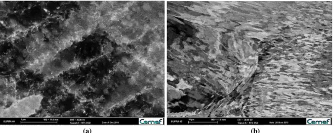
Two Electron Contrast Channeling Imaging (ECCI) micrographs obtained on deformed tantalum samples at different magnifications are presented in Fig. 3. Intragranular lamellar structures are observed. Those are made of dislocation boundaries, consisting of IDBs and GNBs.
5
(a) (b)
Fig. 3. ECCI micrographs on pure tantalum deformed by compression at room temperature up to εVM=0.73.
3. Disorientation gradient calculation from EBSD data 3.1. Presentation of the method
EBSD technique allows measuring the crystal orientation at each measurement point on the sample surface. Hence, the disorientations θi,j can be calculated between any two measurement points i and j. The
presence of dislocations in a deformed crystal may induce a measurable lattice rotation (hereafter referred to as intragranular misorientation). The contribution of the elastic field to the local misorientations can be considered negligible
[23]
so that the local misorientation can be directly linked to, or converted into, a dislocation density. More precisely, a measured misorientation angle (disorientation) can be converted into a number of dislocations that are necessary for accommodating the actual lattice rotation, in other words into a density of GNDs, ρGND. Inorder to determine the dislocation density at each measurement point, the local disorientation θi,j is averaged over
the neighboring points located at a fixed distance x from the pixel of interest. This local average disorientation <θ(x)> is the well-known KAM value (Kernel Average Misorientation angle proposed by all EBSD data processing software packages), provided that the KAM is calculated using only the peripheral pixels and not all the pixels included in the kernel.
A number of studies [14,15,24–31,19] indeed proposed to determine ρGND from EBSD data based either
on the determination of the Nye’s tensor [1] components or on the Read and Shockley representation of low angle boundaries
[32]
using the following equation:,
bx
GND
(4)with α a constant that depends on the type of dislocations, tilt or twist, and x is the distance along which the disorientation <θ(x)> is calculated (Kernel radius if KAM is used). It has been shown in a recent study
[33]
that using Nye’s tensor leads to Eq. (4) with α=3.Despite the frequent use of EBSD for estimating ρGND, major drawbacks have been pointed out. The
usual accuracy of the EBSD technique for determining the crystal orientation lies typically in the range of 0.5-1°. If a dislocation density is calculated from the raw data, the orientation fluctuations related to the measurement noise are converted into a virtual dislocation density as well as the real physical misorientations. This leads to an overestimation of the GND density. The number of GNDs is related to the disorientation, it must be divided by the distance along which the disorientation <θ(x)> is calculated (Kernel radius if KAM is used), see Eq. (4), to get a GND density value. The GND densities estimated that way are thus in addition very sensitive to the step size
[14,34]
, and the overestimation due to the measurement noise is drastically increased when decreasing the EBSD map step size. A simple method used for avoiding this is to take into account only the disorientation6
values that are above a threshold, supposedly representative of the noise level in the data set and typically taken between 0.5° and 1.5° [18]. The choice of the threshold value, of course, also influences the resulting GND density value [14,17,18].
Few years ago, Kamaya
[21]
proposed an elegant method for estimating the measurement noise. This method was used by the present authors to estimate the GND density from <θ(x)> values in cold-deformed tantalum [15], using some functionalities of the MTEX toolbox [35].The method is illustrated below using the EBSD map of Fig. 2a. <θ(x)> values have been calculated for each pixel of the map using the ith neighbors (i = 1 to 5). If the disorientation gradient is constant around the considered pixel, at least within the exploited neighborhood, the <θ(x)> value should be proportional to the distance to the considered neighbor xi; this is the basic principle of the method.
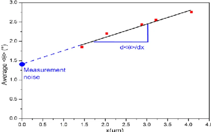
Fig. 4. Average <θ(x)> with 15° upper threshold as a function of the kernel radius (1st to 5th neighbors) calculated on an EBSD map of pure Tantalum deformed to εVM=0.73.
Within the illustrative example shown here, the individual <θ(x)> values have been averaged to get one single average value representative for the whole map. Only disorientation values <θ(x)> below 15° are taken into account in the calculation in order to exclude grain boundaries from the analysis. The averaged <θ(x)> values are presented on Fig. 4 as function of the radius of the considered neighborhood. The averaged value of <θ(x)> is indeed increasing linearly with the Kernel radius; the hypothesis of a constant disorientation gradient within the explored neighborhood around each pixel can thus be considered to be fulfilled. However, this linear variation is not the expected proportionality. Without any measurement noise, the local disorientation should tend to zero when extrapolating the <θ(x)> values to x = 0. In the case of Fig. 4, <θ(x=0)> equals 1.4°, which can be considered as an estimate of the measurement noise
[15,21]
. Another interesting observation is that the disorientation gradient d<θ>/dx is assessed directly from the Kayama's plot, with little influence of the step size or of the neighborhood size (within a reasonable variation range). Indeed it is clear from Fig.4, that the estimated disorientation gradient would be similar if the step size would have been doubled for example (i.e. one point out of two omitted in the plot), or if the neighborhood would have been limited to 3µm. The influence of the step size, or more generally of the pixel-to-pixel distance, is thus reduced when analyzing disorientation gradients instead of disorientations.Replacing <θ>/x in Eq. (4) with d<θ>/dx leads to Eq. (5) which allows a ρGND calculation without the
measurement noise artifact and with a decreased influence of the step size.
.
dx
d
b
GND
(5)The later statement is of course no longer valid if the linear gradient assumption is not fulfilled at the scale of the explored neighborhood. This method can be applied for each pixel of an EBSD map, so that the measurement noise and disorientation gradient d<θ>/dx can be locally assessed and eventually mapped.
7
One advantage of the above described method is that it allows estimating the measurement noise at each point of an EBSD map. As pointed out in different studies [14,16–18], a lower threshold value should be used when calculating a dislocation density from the <θ(x)> values to account for the measurement noise, but then the measurement noise is considered homogenous in all conditions. This value is in general taken between 0.5° and 1.5° [18]. The average values of measurement noise calculated from the EBSD maps presented in Fig. 2 are given in Table 1. It is clear from these values that the measurement noise is not the same for the five considered cases. This observation points out that a fixed value of lower threshold is not the perfect solution. The measurement noise increases when increasing strain, because the distortions of the crystal lattice induced by the presence of an increasing dislocation density affect the quality of the diffraction patterns. The latter become more and more blurred, the Kikuchi band detection less and less accurate, and so goes for the accuracy of the determined orientation. εVM=0.1 εVM=0.16 εVM=0.32 εVM=0.53 εVM=0.73 Average measurement noise 0.4° 0.5° 0.6° 1.1° 1.4°
Table 1. Average measurement noise in the EBSD maps of Fig. 2, determined using the method presented in
section 3.1.
The measurement noise also varies significantly within a single map. Of course, the measurement noise is sensitive to the local dislocation density, but it is also sensitive to the crystal orientation itself, as demonstrated below using an EBSD map of a partially recrystallized pure Tantalum (Fig. 5a). The measurement noise map (Fig. 5b) clearly shows significant differences from one recrystallized grain to another. The dislocation density is expected to be the same in all recrystallized grains, and very low. The difference in the measurement noise inside the different recrystallized grains is thus mainly due to the crystal orientation. This dependence of the measurement noise to the crystal orientation can be explained with the following reasoning: depending on the probed crystal orientation, the Kikuchi bands constituting the analyzed EBSD pattern can be more or less intense and sharp. Lower intensities lead to a poorer accuracy of the detection of the band positions. Thus, the orientation accuracy is potentially better for the orientations leading to a Kikuchi pattern with intense bands. This analysis can be confirmed by comparing the measurement noise to the Mean Angular Deviation (MAD), which is the average value of the angular misfit between each detected Kikuchi bands and the corresponding simulated ones for the estimated orientation. We can observe that the estimated measurement noise (Fig. 5b) varies similarly to MAD parameter (Fig. 5c). In the example of Fig. 5, some of the recrystallized grains, because of their unfavorable orientation, exhibit a measurement noise that is higher than the one of some of the deformed areas, with a favorable orientation and a reasonable dislocation density. In addition, even though it is out of the scope of the present paper, it is worth mentioning that the measurement noise is also likely to be dependent on the algorithm used for band detection and pattern indexing, and thus on the EBSD data acquisition software used. A detailed analysis of the error and precision of the crystallographic orientations and disorientations obtained by EBSD can be found in [36].
The example of Fig. 5 definitely demonstrates that applying a unique threshold value to cutoff the measurement noise in an EBSD map leads to incorrect values of the local GND densities. The estimation of the measurement noise with an objective criterion like with the method applied here presents a real step forward since the noise contribution can be estimated for each individual pixel.
8
(a) (b) (c) (d) (e)Fig. 5. (a) Orientation color-coded EBSD map of a partially recrystallized Tantalum acquired with a step size of
105 nm (normal direction to the analyzed section projected onto the standard triangle, same inverse pole figure color-code as in Fig. 2. (b) measurement noise map obtained using the method described in section 3.1, (c) mean angular deviation map, (d) <θ(x)> map (1st neighbors ; 15° upper threshold) and (e) Disorientation gradient
d<θ>/dx map.
Furthermore, Fig. 5d shows that the recrystallized grains do not have the same <θ(x)> values either. This observation is not physical; it is due to the fact that <θ(x)> does not take into account the measurement noise which is not the same in the different recrystallized grains as already demonstrated in Fig. 5b. The variations in the <θ(x)> values of the recrystallized grains indeed follow the variations in the measurement noise. On the contrary, the recrystallized grains have almost the same disorientation gradient value d<θ>/dx. The comparison between Figs. 5d and 5e obviously exhibit the advantage of using d<θ>/dx instead of <θ(x)>/x to get dislocation densities from EBSD data, since those two parameters are proportional to ρGND as pointed out in
9
The values of ρGND associated to the red squares on Fig. 5a are calculated using <θ(x)> associated to Eq.
(4) and d<θ>/dx associated to Eq. (5) and summarized in Table 2. The effect of considering the measurement noise is clearly observed, especially in the case of recrystallized region. The use of <θ(x)> to estimate ρGND leads
to overestimated values. Using <θ(x)> Using d<θ>/dx Deformed region 1.41015 m-2 7.91014 m-2° Recrystallized region 9.11014 m-2 5.71013 m-2
Table 2. Average ρGND associated to the red squares on Fig. 5a are calculated using <θ(x)> associated to Eq. (4)
and d<θ>/dx associated to Eq. (5).
Thus, the use of d<θ>/dx and Eq. (5), instead of <θ(x)>/x and Eq. (4), will give a more accurate distribution of ρGND (qualitatively similar to Fig. 5e and 5d respectively), accounting from measurement noise.
Another major drawback of the quantitative analysis of dislocations with EBSD data is the step size dependence. The determination of GND from disorientations measured by EBSD data, either using Nye’s tensor
or eq. (4), always depends on the step size acquisition. Provided that the step size is well adapted to the microstructure scale (i.e. that the disorientation gradients are constant within the exploited local neighborhood), the influence of the step size is decreased by using the disorientation gradients. This is another advantage of the proposed method.
Remark 1: The presented method is applied using <θ(x)> with an upper threshold value of 15° so that the grains
boundaries are not considered in the calculations. This can lead to some apparent saturation of disorientations <θ(x)>, and therefore of disorientation gradients d<θ>/dx, as already pointed out by Pantleon [17]. For the studied equivalent strains (maximum εVM= 0.73) this threshold value will not
lead to such saturation because only few intragranular disorientations are observed above that value (few black lines inside grains of Fig. 2e). But for higher strain levels, this upper threshold value should be reconsidered. On the other hand, it is clear from Fig. 2 that some of the boundaries delimiting the grains of that material have disorientation below 15° (not plotted black). Those boundaries will be included in the analyses below.
Remark 2: For some pixels, no clear gradient is observed. In fact, for regions with very small distortions of the
crystal lattice (for ex. recrystallized grains), very weak disorientation gradients d<θ>/dx should be obtained. In such regions, the measured crystal orientation fluctuates within the measurement noise and a nonsensical negative d<θ>/dx value can be obtained. Such odd values are set to zero. In other words, when the disorientation is smaller than the measurement noise, no disorientation gradient can be detected so we consider that there are no dislocations.
4. Statistical analysis of IDBs and GNBs from EBSD data 4.1. Method presentation
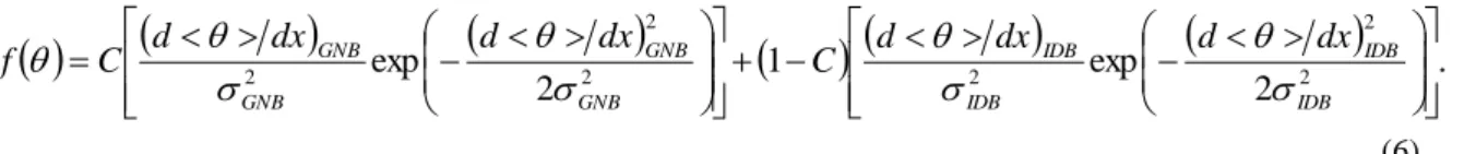
Experimental probability density distribution of disorientations or of disorientation gradients can be obtained from EBSD data, including both IDBs and GNBs. Eq. (3) allows then to determine the probability density distribution of disorientations of IDBs and of GNBs separately and the fraction of each. As already mentioned above, disorientation gradients will be used here instead of disorientations, Eq. (3) becomes:
.
2
exp
1
2
exp
2 2 2 2 2 2
IDB IDB IDB IDB GNB GNB GNB GNBd
dx
C
d
dx
d
dx
dx
d
C
f
(6) Hence, accumulated frequency can be described by the following equation:10
.
2
exp
1
1
2
exp
1
2 2 2 2
IDB IDB GNB GNB d accumulatedx
d
C
dx
d
C
f
(7)Fitting Eq. (6) or (7) with experimental probability densities of d<θ>/dx obtained from EBSD allows determining σIDB, σGNB and C. This way, the distribution functions of d<θ>/dx of IDBs and GNBs, and the
fraction of each are determined. These three parameters allow a quite good statistical description of the dislocation structures.
The main assumption behind the present method is that the value d<θ>/dx of each pixel is attributed to the presence of IDBs or GNBs. This assumption is realistic only when the acquisition step size (here 1.41µm) is bigger than the magnitude of the spacing of GNBs or IDBs. For every pixel, d<θ>/dx was calculated within a square of 55 pixels centered on the pixel of interest. If no GNB or IDB is within this square, no significant disorientation gradient is detected (lower than the measurement noise) and the value of d<θ>/dx is set to zero. If several GNB or IDB are present within the square of 55 pixels, d<θ>/dx value will account for their cumulative effect. However, dislocation boundaries may exhibit orientation fluctuations leading to no disorientation gradient at the scale of the step size. Those dislocation boundaries cannot be detected with the present approach.
4.2. Results
Pure tantalum is a BCC material with a relatively high stacking fault energy [37–39] making the out of gliding plane movement of dislocations easier.5
For a given EBSD map consisting of a total number of pixels Ntot, the disorientation gradient d<θ>/dx
values obtained from the EBSD maps for each pixel were gathered into bins of width
µm
dx
d
/
0035
.
0
(1000 bins minimum). Ni stand for the number of pixels within each bin i and
N
iN
is the total number of pixels with d<θ>/dx>0.The complementary part N0 (= Ntot – N) corresponds to pixels where the disorientation gradient is set to
zero because below the measurable limit of the current approach. It is worth mentioning that in the previous works by Pantleon and Hansen, which were based on TEM measurements, only locations with a visible dislocation boundaries have been considered. Areas without significant dislocation content have thus not been taken into account at all in the performed analyses. Here, starting from EBSD data, those areas can be quantified (their surface fraction is simply given by the ratio N0/Ntot), even though they will be excluded when quantifying
IDBs and GNBs, to be fully consistent with former works. Hence, experimental probability density distributions of disorientation gradient can be calculated as follow:
.
dx
d
N
N
P
i i
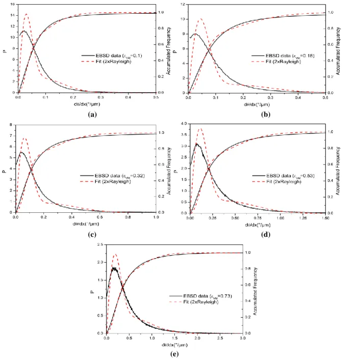
(8)Fitting experimental probability density distributions to the ones predicted by the model (Eq. (6)) allows identifying the 3 parameters of the model with a least square minimization using a generalized reduced gradient method. Experimental probability density distributions and accumulated frequencies of d<θ>/dx are compared to the theoretical model given in Eq. (6) and (7) on Fig. 6.
The “double” Rayleigh distribution of Eq. (6) and (7) provides a satisfactory description of the experimental results, especially for the accumulated frequency plots. Even though the agreement is not exactly perfect, it is as satisfactory as it was for the previous comparisons with TEM data [12,13].
The results presented on Fig. 6 also suggests that the mathematical form previously proposed [13] for analyzing TEM data is also suitable for EBSD data. The mismatch is greater for smaller εVM values. This is
somehow expected, since IDBs and GNBs may not be formed at such low deformation level and since all detected d<θ>/dx are assumed to be induced by IDBs or GNBs in the present method. On the other hand, for the
11
highest considered εVM value (0.73), the agreement between the experimental d<θ>/dx distribution and the
Rayleigh model is quite good, even though it is very likely that all the GNBs and IDBs have not been measured individually with the current EBSD map step size. Optimizing the EBSD step size according to the microstructure scale remains an opened question that would deserve a complete dedicated study. However, the possibility of describing quite well the disorientations measured by EBSD with the same tools used for TEM data, opens a new route for the quantitative analysis of deformation substructures.
(a) (b)
(c) (d)
(e)
Fig. 6. Experimental probability densities of disorientation gradient and accumulated frequencies in comparison
with the theoretical model presented in Eq. (6) and (7) respectively (a) εVM=0.1, (b) εVM=0.16, (c) εVM=0.32, (d) εVM=0.53 and (e) εVM=0.73.
This fitting procedure allows determining σIDB and σGNB, and the frequencies of each (considering only
non-null values of d<θ>/dx). For an easy interpretation of the results
d
dx
IDB and
d
dx
GNB, calculated using Eq. (2), are presented in Table 3. We should mention that with σIDB and σGNB the probability12
εVM=0.1 εVM=0.16 εVM=0.32 εVM=0.53 εVM=0.73
Experimental
d
dx
(°/µm) 0.08 0.12 0.17 0.29 0.43Double Rayleigh Distribution
d
dx
(°/µm) 0.07 0.1 0.15 0.27 0.42
d
dx
GNB(°/µm) 0.12 0.21 0.31 0.51 0.71
d
dx
IDB(°/µm) 0.04 0.04 0.08 0.13 0.23C 0.39 0.31 0.33 0.37 0.4 Frequency of pixels with
d<θ>/dx = 0 29% 25% 19% 18% 15%
Table 3. Average values of the experimental disorientation gradients
d
dx
and of the modeled ones for IDBs and GNBs. Relative frequency C of GNBs among all dislocation boundaries (parameters of Eq. (6) and (7)), and frequency of the pixels with a disorientation gradient below the detection limit (set to 0).4.3. Discussion
The satisfactory correlation of experimental EBSD results with a double Rayleigh distribution means that dissociation of IDBs and GNBs can also be possible from EBSD data. The average values of
d
dx
(including all dislocation boundaries, IDBS and GNBs, i.e. all positive values of d<θ>/dx) obtained from EBSD data and presented in the first line of Table 3 are close to the ones obtained from Eq. (6) after fitting.
The frequency of pixels for which no reliable d<θ>/dx could be measured (because smaller than the measurement noise), i.e. those with low dislocation densities and disorientation gradients, decreases with increasing εVM as expected.
The frequency of GNBs among all dislocation boundaries, i.e. the C parameter, does not vary much with strain. The values of C presented in Table 3 are in good agreement with previous results [13] from the literature obtained on cold-rolled aluminum up to 50% reduction. Conversely, the amplitude of the disorientation gradients associated with GNBs is drastically increasing with strain.
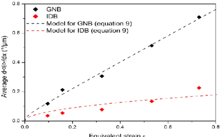
The average values of
d
dx
GNB and
d
dx
IDB, also given in Table 3, are plotted in Fig. 7 as a function of εVM. Pantleon [17,40] developed a semi-empirical model to describe the evolution of thedisorientation θ as a function of strain for GNBs and for IDBs in aluminum alloys:
(9)
where P is the immobilization probability, b is the magnitude of the Burgers vector, d* is a disorientation correlation length and σimb is an activation imbalance to account for the additional deterministic contribution
characterizing GNBs. This model was originally developed to describe the evolution of average disorientation
and will be tested below on the average disorientation gradient
d
dx
data of GNBs and of IDBs. The parameters AIDB, AGNB and B are identified by least square fitting Eq. (9) with the experimental results, as shownin Fig. 7. For both GNBs and IDBs the comparison is quite satisfactory. However, the strain levels considered here are relatively small, so it is difficult to draw definite conclusions regarding the validity of Pantleon’s model (of Eq. (9)) applied to EBSD data without studying higher strains.
2 2 2 * *
2
2
B
A
d
Pb
A
d
Pb
GNB imb GNB GNB IDB IDB IDB
13
Fig. 7. Evolution of the average disorientation gradient d<θ>/dx of IDBs and GNBs as a function of equivalent
strain. Comparison between experimental results and Pantleon’s model predictions, Eq. (9).
As already mentioned, using the disorientation gradient d<θ>/dx allows for overcoming in great part the EBSD measurement accuracy issue, notably for erasing the influence of the crystal orientation on the measurement noise, and to some extent to vanish the sensitivity of the analysis to the step size. In view of a real quantitative analysis of the dislocations substructures, the step size must be chosen properly. Further work is required to learn how to optimize the EBSD step size, notably with regards to the spacing the dislocation boundaries, but more generally with regards to the scales of the different microstructure features.
In addition, analyzing GNBs and IDBs from EBSD data, does not necessarily mean that all dislocation boundaries present within the surface analyzed by EBSD must be considered. Within the present settings, only some of them have probably been detected and analyzed, but the resulting disorientation gradient distributions could nevertheless be fitted with the same models applied to TEM data. Hence, the present method should not be considered as a direct and quantitative analysis but more as a semi quantitative statistical analysis. Using TEM to analyze IDBs and GNBs allows studying exhaustively all dislocation boundaries within a very small surface (up to few hundreds of µm²), using EBSD allows studying statistically some of the dislocation boundaries within a large surface (up to few mm²). In that sense, EBSD cannot replace TEM for analyzing dislocation boundaries, but can add additional statistical information, and thus provides a means of verifying if the tendencies observed on a small surface are the same on larger ones.
5. Conclusion
The description of dislocations structure is discussed in the present paper in terms of dislocations boundaries IDBs and GNBs. The concept of considering dislocations as parts of dislocation structures (sub-boundaries) has indeed been proposed and developed since several years. The Rayleigh distribution function was observed to be a good descriptor of the distribution function of the disorientation associated with individual sub-boundaries. However, to our knowledge, this was only established using TEM data.
Here EBSD data are used to identify parameters for the quantitative description of dislocations boundaries instead of TEM data in former works. EBSD data have the advantage of providing a better statistical relevance as compared to TEM data, but also have a major drawback regarding the contribution of the measurement noise to the local misorientations from which dislocation densities and sub-boundaries can be assessed. This drawback could be overcome using Kamaya's approach which allows for estimating the measurement noise at any point of an EBSD map. The measurement noise appears to be strongly affected by the presence of dislocations and by the orientation of the crystal lattice itself. Furthermore, as already pointed out in the literature, local disorientations measured in EBSD maps, and consequently the deduced dislocation densities, are greatly influenced by the step size. In order to reduce the step size influence, the disorientation gradient
d<θ>/dx, also derived from the Kamaya's plot, was used as a parameter to replace the disorientation <θ> to
characterize dislocation boundaries.
The distribution functions of local disorientation gradients d<θ>/dx obtained from EBSD data on (BCC) pure Tantalum could also be described with Rayleigh functions. The distribution functions of GNBs and of IDBs separately and the frequency of each type of dislocation boundaries were calculated from the overall disorientation gradient distribution, following the same principle applied formerly by Hansen and Pantleon on
14
TEM disorientation data. The proportion of GNBs among all dislocation boundaries appeared to be stable (around 35%) within the investigated strain range (0.1 to 0.73). The disorientation gradients corresponding to each type of dislocation boundaries increase with strain, but GNBs evolve faster than IDBs. This is in full agreement with the state of the art conclusions.