HAL Id: hal-02943467
https://hal.archives-ouvertes.fr/hal-02943467
Submitted on 19 Sep 2020
HAL is a multi-disciplinary open access
archive for the deposit and dissemination of
sci-entific research documents, whether they are
pub-lished or not. The documents may come from
teaching and research institutions in France or
abroad, or from public or private research centers.
L’archive ouverte pluridisciplinaire HAL, est
destinée au dépôt et à la diffusion de documents
scientifiques de niveau recherche, publiés ou non,
émanant des établissements d’enseignement et de
recherche français ou étrangers, des laboratoires
publics ou privés.
ANALYSIS OF COMMON DESIGN CHOICES IN
DEEP LEARNING SYSTEMS FOR DOWNBEAT
TRACKING
Magdalena Fuentes, Brian Mcfee, Hélène Crayencour, Slim Essid, Juan Bello
To cite this version:
Magdalena Fuentes, Brian Mcfee, Hélène Crayencour, Slim Essid, Juan Bello. ANALYSIS OF
COM-MON DESIGN CHOICES IN DEEP LEARNING SYSTEMS FOR DOWNBEAT TRACKING. The
19th International Society for Music Information Retrieval Conference, Sep 2018, Paris, France.
�hal-02943467�
SYSTEMS FOR DOWNBEAT TRACKING
Magdalena Fuentes
1,2,∗, Brian McFee
3,4, H´el`ene C. Crayencour
1, Slim Essid
2, Juan P. Bello
3 1L2S, CNRS-Univ.Paris-Sud-CentraleSup´elec, France
2
LTCI, T´el´ecom ParisTech, Univ. Paris-Saclay, France
3Music and Audio Research Laboratory, New York University, USA
4
Center of Data Science, New York University, USA
ABSTRACT
Downbeat tracking consists of annotating a piece of mu-sical audio with the estimated position of the first beat of each bar. In recent years, increasing attention has been paid to applying deep learning models to this task, and various architectures have been proposed, leading to a significant improvement in accuracy. However, there are few insights about the role of the various design choices and the delicate interactions between them. In this paper we offer a system-atic investigation of the impact of largely adopted variants. We study the effects of the temporal granularity of the in-put representation (i.e. beat-level vs tatum-level) and the encoding of the networks outputs. We also investigate the potential of convolutional-recurrent networks, which have not been explored in previous downbeat tracking systems. To this end, we exploit a state-of-the-art recurrent neural network where we introduce those variants, while keeping the training data, network learning parameters and post-processing stages fixed. We find that temporal granularity has a significant impact on performance, and we analyze its interaction with the encoding of the networks outputs.
1. INTRODUCTION
Musical rhythm is organized into hierarchical levels which interact with each other. One of the predominant pulsa-tions is the beat, which matches the foot tapping of a per-son when listening to a music piece. Tatum is related to the fastest pulsations still perceived by listeners, usually twice to four times faster than beat. Beats of different accentuations are grouped in bars. Automatic downbeat tracking aims to determine the first beat of each bar, being a key component for the study of the hierarchical metri-cal structure. It is an important task in Music Information Retrieval (MIR) that represents a useful input for several applications, such as automatic music transcription [19], structural segmentation [18] and rhythm similarity [22].
c
Magdalena Fuentes, Brian McFee, H´el`ene C. Crayen-cour, Slim Essid, Juan P. Bello. Licensed under a Creative Commons Attribution 4.0 International License (CC BY 4.0). Attribution: Mag-dalena Fuentes, Brian McFee, H´el`ene C. Crayencour, Slim Essid, Juan P. Bello. “Analysis of Common Design Choices in Deep Learning Systems for Downbeat Tracking”, 19th International Society for Music Informa-tion Retrieval Conference, Paris, France, 2018.
The task of downbeat tracking has received considerable attention in recent years. In particular, the introduction of deep neural networks provided a major improvement in the accuracy of downbeat tracking systems [3, 10, 16], and the systems relying on deep learning have become the state-of-the-art. These approaches usually exploit a first stage of low-level feature computation, where several rep-resentations such as chroma [10] or spectral flux [16] have been adopted. This is usually followed by a stage of fea-ture learning with neural networks, whose outcome is an activation function that indicates the most likely candi-dates for downbeats among the input audio observations. Then, a post-processing stage is often used, which con-sists of a dynamic model, typically a Dynamic Bayesian Network (DBN), Hidden Markov Model (HMM) or Con-ditional Random Field [4, 11, 12].
Among the mentioned systems, different design choices were taken at different stages of the processing pipeline, such as the temporal granularity of the input, low-level feature representations, network architecture, and the post-processing methods. Additionally, different proposals were evaluated using distinct training data and/or evalu-ation schemes (e.g., cross-validevalu-ation vs leave-one-dataset-out) [4, 11, 16]. This variability makes it difficult to gain insights about the actual role of each design choice, and the delicate interactions between them.
In this paper, we systematically investigate the impact of design choices in downbeat tracking models. In par-ticular, we study the effect of temporal granularity of the input representation (i.e., beat-level vs tatum-level), the output encoding (i.e., the label encoding used to train the networks), and their interactions with the post-processing stage and internal network architecture. This allows for gaining fresh understanding into the potential and limita-tions of the state-of-the-art approaches, and takes a step toward the systematic design of these systems.
1.1 Related work
Durand et al. [11], proposed a system for downbeat track-ing that consists of an ensemble of models each represent-ing four different aspects of music: rhythm, harmony, bass content and melody. The authors developed a Convolu-tional Neural Network (CNN) for each musically inspired representation, and estimated the downbeat likelihood by
averaging the likelihoods produced by each CNN in the en-semble. Then, the authors turn the soft state assignments of the CNN ensemble into hard assignments (downbeat vs no-downbeat) using an HMM. This approach showed the potential of CNNs for downbeat tracking and the comple-mentarity of the different musically inspired features.
In parallel, B¨ock et al. [4], presented a system that jointly tracks beats and downbeats using Bi-Directional Long-Short Term Memory networks (Bi-LSTMs). The authors used three different magnitude spectrograms and their first order differences as input representations, in or-der to help the networks capture features with sufficient resolution in both time and frequency. The input represen-tations were fed into a cascade of three fully connected Bi-LSTMs, obtaining activation functions for beat and down-beat as output. Subsequently, a highly constrained DBN was used for inferring the metrical structure.
In turn, Krebs et al. [16] proposed a downbeat track-ing system that uses two beat-synchronous features to rep-resent the percussive and harmonic content of the audio signal. Those feature representations, based on spectral flux and chroma, are then fed into two independent Bidi-rectional Gated Recurrent Units (Bi-GRUs) [8]. Finally, the downbeat likelihood is obtained by merging the likeli-hoods produced by each Bi-GRU. The final inference for downbeat candidates relies on a constrained DBN.
More recently, combinations of CNNs and Recurrent Neural Networks (RNNs) such as GRUs or LSTMs have received increasing attention. For instance, Convolutional-Recurrent Neural Network architectures (CRNNs) have been proposed in other MIR tasks such as chord recogni-tion [20] or drum transcriprecogni-tion [23], and they are the state of the art in other audio processing domains such as sound event detection [2, 6].
1.2 Our contributions
In this paper we offer a systematic investigation of impor-tant system design choices, namely the impact of the in-put observations’ temporal granularity, the outin-put encod-ing, and the post-processing stage. Also, we investigate the potential of CRNNs for improving feature learning for the task of downbeat tracking. To perform our experiments, we modify a state-of-the-art RNN-system [16], and study the effect of the different envisaged variations, keeping the training setup and input features fixed. Our experimental results show that the post-processing stage improves the performance in all cases, whereas the addition of a dense-structured output encoding does not help in the training of downbeat tracking systems. The proposed CRNN ar-chitecture performs competitively with the state-of-the-art RNN system, being even able to improve the reference sys-tem’s performance with a proper choice of input’s temporal grid. We also observe that though beat tracking errors tend to propagate to the output decisions, the CRNN system is able to recover from these errors better than the baseline RNN when taking the input observations over a tatum grid (as opposed to beat grid).
2. ANALYSIS OF COMMON VARIATIONS In this section we briefly describe the baseline system, the motivation of each studied variation (or design choice) and the experiments related to it. In particular, we study the ef-fects and interactions of 4 design choices: the input’s tem-poral granularity, the output encoding, the effect of post-processing and the network architecture.
2.1 Recurrent neural network baseline
To perform our analysis, we implemented the state-of-the-art downbeat tracking system presented by Krebs et al. [16]. The architecture of this system consists of two concatenated Bi-GRUs of 25 units each, where each hid-den state vector h(t) at time t is mapped by a hid-dense layer to a state prediction p(t) using a sigmoid activation. A dropout layer is used in training to avoid over-fitting. Two separate networks are trained using different input features and the obtained likelihoods are averaged. The low-level input representations comprise two beat-synchronous fea-ture sets, representing the harmonic and percussive con-tent of the audio signal. The set of features describing percussive content, which we will refer to as PCF (Per-cussive Content Feature), is based on a multi-band spectral flux, computed using the short time Fourier transform with a Hann window, using a hop-size of 10ms and a window length of 2048 samples, with a sampling rate of 44100 Hz. The obtained spectrogram is filtered with a logarithmic fil-ter bank with 6 bands per octave, covering the range from 30 to 17 000 Hz. The harmonic content’s representation is the CLP (Chroma-Log-Pitch) [21] with a frame rate of 100 frames per second. The temporal resolution of the features is 4 subdivisions of the beat for the PCF, and 2 subdivi-sions for the CLP features. For computational efficiency, the authors in [16] assembled in matrices column-wise this resolution increment so the CLP feature set is of dimension 12 × 2 and the PCF is 45 × 4, which we maintained in this work. The beats for the beat-synchronous feature mapping are obtained using the beat tracker presented in [3], with the DBN introduced in [17].1
In our experiments, we have observed that including batch normalization (BN) layers [14] consistently im-proves performance. We included two BN layers, one after the input layer, and the other between the Bi-GRUs.
The optimization of the model parameters is carried out by minimizing the binary-cross-entropy between the esti-mated and reference values.
2.2 Temporal granularity: beat vs tatums
The temporal granularity of the input observations (or tem-poral grid) relates to important aspects of the design of downbeat tracking systems. It determines the length of the context taken into account around musical events, which controls design decisions in the network architecture, such as filter sizes in a CNN, or the length of training sequences in an RNN.
1In particular we used the DBNBeatTracker algorithm of the madmom
package version 0.16 [5].
Among the different downbeat systems, several granu-larities have been used. In particular, the latest state-of-the-art systems use either musically motivated temporal grids (such as tatums or beats) or fixed length frames. Systems that use beat- or tatum-synchronous input depend on reli-able beat/tatum estimation upstream, so they are inherently more complex, and prone to error propagation [11, 16]. On the other hand, frame-based systems are not subject to these problems, but the input dimensionality is much higher due to the increased observation rate [4], which causes difficulties when training the models.
In this paper, we focus on musically motivated tempo-ral analysis grids, because they reduce the computational complexity of the systems considerably. We study the vari-ations in performance using beat and tatum grids.
We compute the tatums by interpolating the beats, with a resolution of 4 tatums per beat interval.2 To study the
impact of the temporal grid, we train the networks keep-ing the input features, architecture, trainkeep-ing data, and post-processing fixed, while changing only the inputs’ temporal granularity. We adapt the sequence length used for training the networks in order to consider the same musical context in all cases (as specified further below). We compare the interaction of the choice of temporal grid with those of the output encoding, the RNN or CRNN architectures and the post-processing stage.
2.3 Output encoding: structured vs unstructured Among the downbeat tracking systems mentioned in Sec-tion 1.1, the common choice is to use an one-hot vector encoding to indicate the presence or absence of a down-beat at a particular position of the excerpt at training time. For instance, if using temporal analysis grid that is aligned on beats, a sequence of beats is usually encoded as s = [1, 0, 0, 0, 1, 0, 0, 0], indicating the presence of a downbeat at the first and 5th beat positions. We refer to this as un-structuredencoding. Here, we also investigate whether a densely structured encoding may help the neural networks perform a better downbeat tracking.
2.3.1 Structured encoding definition
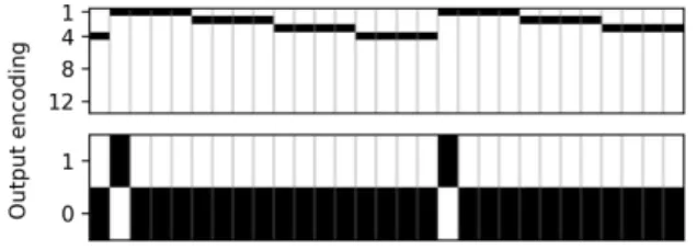
We define the structured encoding as a set of classes that are active within the entire inter-beat interval. This is the set C = {1, . . . , 13}, where each class indicates the po-sition of the beat inside a bar. We consider a maximum bar length of 12 beats, and an extra class X for labeling an observation in the absence of beats and downbeats, for a total of 13 classes (K = 13). For instance, to label a mu-sical piece with time signature 4/4, we use the subset of labels {1, 2, 3, 4}, and we label consecutive time units cor-responding to the same beat interval with the same class. Figure 1 illustrates the difference between the proposed and the unstructured encoding. In this strutured class lex-icon, the downbeats are represented by the label 1.
We train the networks incorporating both the unstruc-tured and the strucunstruc-tured encoding. In this configuration,
2This estimation is on the 16th note level, which we assumed as a
good compromise to perform downbeat tracking.
Figure 1. Audio excerpt in 4/4 labeled with the struc-turedencoding (top figure) and the unstructured encoding (bottom figure). The temporal granularity showed is tatum (beat quarter-notes). In the structured encoding each tatum receives a label corresponding to its metrical position.
we use one dense layer to decode each class lexicon, and we evaluate the performance of the system using the un-structured output. The dense layers are connected so the information of the beginning of the bar is provided by the unstructured dense to the structured one as an extra fea-ture. We test the effect of the encoding on the different temporal granularities. It is important to note that the un-structured coding has a clear interaction with the temporal grid in terms of the number of 1- vs 0- symbols in the train-ing data , while the structured codtrain-ing is consistent (i.e., the amount of class instances remains proportional) under any temporal granularity.
2.4 Post-processing: DBN vs thresholding
The importance of the post-processing stage has been ad-dressed in previous works [11, 16]. In this paper, we assess the relative importance of this stage depending on the tem-poral granularity and the network architecture. To that end, we use the DBN presented in [16]. This DBN models beats (or tatums) as states, forcing the state sequence to always transverse the bar from left to right (i.e., transitions from beat 2 to beat 1 are not allowed), and imposing that time signature changes are unlikely. We consider bar lengths of 3 and 4 beats (12 and 16 tatums). We invite the interested reader to refer to [16] for further information.
2.5 Architecture: RNNs vs CRNNs
We base our CRNN architecture design on previous state-of-the-art choices. Particularly, our CNN design is based on the best CNN of the ensemble in [11], which we com-bine with a single Bi-GRU layer [8]. The bi-directional version of GRUs integrates the information across both temporal directions, providing temporal smoothing. CNNs are capable of extracting high level features that are in-variant to both spectral and temporal dimensions, whether RNNs model longer term dependencies accurately.
The architecture that we propose can be seen as an encoder-decoder system [7], where the encoder maps the input to an intermediate time series representation that is then mapped to the output space by the decoder. An in-teresting advantage of this kind of scheme is that several combinations of encoder-decoder can be explored easily as long as they share the intermediate representation.
Figure 2. Encoder architecture: the input representation is either a beat/tatum-synchronous chromagram or multi-band spectral flux. Each time unit is fed into the encoder with a context window. The CNN outputs a sequence of dimension T × N which is fed to the Bi-GRU. Finally, the encoder output dimension is T × 512.
Figure 3. Summary of the CNN architecture.
2.5.1 Encoder architecture
The encoder architecture is depicted in Figure 2. It con-sists of a convolutional-recurrent network. Each temporal unit (either beat or tatum) is fed into the CNN considering a fixed-length context window of approximately one bar (following [11]). The CNN processes each window inde-pendently, and outputs a sequence of size T × N (T being the length of the input sequence and N the output dimen-sion of the CNN) that is fed to the Bi-GRU. In this scheme, the CNN processes the signal locally whereas the recurrent network provides temporal consistency.
The CNN architecture is based on the harmonic-CNN presented in [11]. This network consists of a cascade of convolutional and max-pooling layers, with dropout used during training to avoid over-fitting, to a total of eight lay-ers. We add batch normalization layers to avoid too large or small values within the network that could hurt the en-coder. Additionally, we modify the filters’ size to adapt to the feature shapes described in Section 2.1. Figure 3 shows the filter parameters in the case of the tatum grid.
The last layer of the CNN differs from the reference implementation in the number of units, which we set to 13 instead of 2 to fit features of bigger dimension to the Bi-GRU. We also remove the softmax activation of the last layer because the class discrimination is not carried out by the CNN. A summary of the CNN architecture is presented in Figure 3. Figure 3 represents the CNN’s 2D filter sizes and the number of units, which is [m × n, u], with m and n operating in the spectral and temporal dimensions respec-tively, and u the number of units. The activation (if used) is indicated before the CNN description. Max pooling layers are notated as [m0×n0], s indicating frequency and time
di-mension and stride. The interested reader is referred to [11] for the motivation of network architecture.
The local features computed by the CNN are fed into a Bi-GRU, which consists of two independent GRUs, one running in each temporal direction. Their hidden state vec-tors are concatenated to produce the bi-directional hidden state vector. We set the dimensionality of each GRU to 256, resulting in a total of 512.
2.5.2 Decoder architecture
Our decoder architecture is a fully connected dense layer that maps each hidden state vector to the prediction state using a sigmoid activation, resulting in a downbeat like-lihood at each time unit. The optimization of the model parameters is carried out by minimizing the binary-cross-entropy among the estimated and actual values.
3. EXPERIMENTS 3.1 Experimental setup
Model implementation: The models were implemented with Keras 2.0.6 and TensorFlow 1.2.0 [1, 9]. We use the ADAM optimizer [15] with default parameters. We stop training after 10 epochs without changes on the validation set, up to a maximum of 100 epochs. The low-level repre-sentations were extracted using the madmom library and mapped to either the beat or tatum grid (see Section 2.1). Model variations: We study the following variations: Temporal granularity: using low-level features synchro-nized to two temporal granularities (tatum and beat); Output encoding: with and without the addition of the structured encoding during training;
Post-processing: using either a threshold or a DBN; Architecture: we test RNNs and CRNNs.
This results in sixteen different configurations, which we will refer to as and R or C to indicate the architec-ture (RNN vs CRNN); S or U to indicate the encoding (structured vs unstructured); B or T to indicate temporal granularity (beat vs tatum); and t and d to indicate the post-processing method (threshold vs DBN). All models are trained using patches of 15 beats or 60 tatums depend-ing on the temporal grid used. We use mini-batches of 64 patches per batch and a total of 100 batches per epoch. Datasets: We investigate the performance of these config-urations on 8 datasets of Western music, in particular: Klapuriwhich consists of 4h 54m of various genres songs. R. Williamswhich consists of 4h 31m of Pop songs. Rockwhich consists of 12h 53m of Pop and Rock songs. RWC Popwhich consists of 6h 47m of Pop music. Beatleswhich consists of 8h 01m of Beatles songs. Ballroomwhich consists of 6h 04m of Ballroom dances. Hainsworthwhich contains 3h 19m of various genres. RWC Jazz, which consists of 3h 44min of Jazz music. Evaluation methods: We perform leave-one-dataset-out evaluation and report the F-measure scores as in [11, 16]. 25% of the training data is used for validation. The Proceedings of the 19th ISMIR Conference, Paris, France, September 23-27, 2018 109
RWC Jazz dataset is only used to illustrate the performance of the systems in a challenging scenario where the beat es-timation is less accurate and the music genre differs con-siderably from the training data, it is not used for train-ing.3 Candidates for downbeats are obtained in two
dif-ferent manners. The first one is by thresholding the out-put activations with a threshold chosen to give the best F-measure result on the validation set. The second manner is to post-process the networks’ outputs by adapting the DBN used in [16]. In this way we report the gain of us-ing the DBN in each case. We use the DBN to model time signatures 3/4 and 4/4 following [16], and modifying it ac-cordingly to the temporal grid (i.e., allowing bar lengths of {3,4} beats or {12, 16} tatums).
Methods are evaluated independently on each dataset listed above for comparison to prior work. We also in-clude an evaluation over the union of all datasets (denoted ALL). To determine statistically significant differences, we conduct a Friedman test on the ALL-set results, followed by post-hoc Conover tests for pairwise differences using Bonferroni-Holm correction for multiple testing [13].
All configurations are trained with the same input low-level representations, the same musical context, the same training parameters and post-processing method. This al-lows us to draw conclusions about the performance of the models in different conditions and to compare the architec-tures modularly.
3.2 Results and discussion
We use as baseline two state-of-the-art downbeat tracking systems [11, 16], which reported 78% and 78.6% mean F-measure across all datasets.4 The performance of the
models presented here across datasets is better than the baselines for all the cases when using the DBN as post-processing stage. The better results are obtained with RUBd (reference implementation, see Section 2.1) and CUTd up to 82.4% and 82.8% respectively. A possible explanation for this improvement is the difference in the beat tracking performance, which is 3.3% better than the one reported in [16]. This is likely to explain the 4.7% improvement in the RUBd model which is our reference implementation. To make a fair comparison, we use the RUBd model as a baseline, with the reasonable assumption that it behaves as the state-of-the-art. Figure 4 illustrates the performance of the different model variations across datasets. A detailed analysis is presented in the following. The Friedman test on the ALL set rejected the null hypothesis (p < 1e−10). Post-hoc analysis determined that all pair-wise comparisons were significantly different (p < 1e−3), with the following exceptions: RUTt/RSTt, RUTd/RSTd, CUTt/CSBt, CUTd/CSBd, CUBd/CSTd, and RSBd/CUBd.
Effect of post-processing: As shown in Figure 4, d vs t model variants, the DBN post-processing helps in all
3We kept RWC Jazz out of the training set to be comparable to [16]. 4For datasets that are not evaluated in [11], we report results in [16].
cases, being particularly important with the tatum granu-larity and with the RNN models. The gap in performance between the models with and without post-processing is notable in the case of the Ballroom database, where in some cases is up to 10% F-measure. The DBN increases the performance from RUTt to RUTd by 6.6% in the case of tatum grid across all databases, and 4.1% in the case of the beat grid (RUBt to RUBd). A similar trend is observed with the structured models (RS). The increase in the CRNN models performance is smaller, being 3.8% from CUTt to CUTd and 2.7% for CUBt to CUBd. The results obtained with the thresholding (t models) are more consistent over temporal granularities for the CRNN models, which suggests that the likelihood estimation of that model is more accurate and consistent over time. Effect of the temporal granularity: The temporal grid has an important effect on the performance of the RNN models, as illustrated in Figure 4 (T vs B variations). When using a tatum grid, the thresholding results (e.g. RUTt) are lower in most of the cases, showing that the RNN vari-ations have more difficulty to model the temporal depen-dencies in that grid. The post-processing stage with the DBN becomes more important in the case of the tatum grid, helping the RNN models up to an extra 2.5% in mean F-measure over all datasets compared to the beat grid case. By contrast, the CRNN models appear to be robust to the temporal granularity change. In particular, for the case of the thresholding results, the performance of the models is similar for the beat and tatum granularities (e.g. CUBt vs CUTt), which implies the estimated likelihoods perform comparably. The increase in resolution seems to help the CRNN models in most cases, showing a small increase from beat to tatum grid with the DBN (e.g., CUBd vs CUTd). This indicates that the CRNN architecture is likely being able to take advantage of a finer temporal grid.
The impact of the temporal granularity in the RNN and CRNN models are in line with the decisions of the authors in [11, 16], who in the first case decided to use tatums (with CNNs), and in the second case decided to use beats (with Bi-GRUs).
Effect of the structural encoding: Regarding the struc-tural encoding, the experiments show that it has no im-pact on the performance across databases (e.g. RU vs RS and CU vs CS in Figure 4). We observed some examples where the performance decreases, and we noticed two sys-tematic problems: first, in some cases the estimated likeli-hoods become sharper and more structured when using the encoding, and when the estimation of the networks is not accurate the likelihoods consistently maintain the bad esti-mation across the whole duration of the audio signal. This indicates that the encoding is structuring the likelihood es-timation, but that is not desirable in some cases, especially if it prevents the post-processing stages from compensating for these errors. Second, we observed several cases where the attack of the downbeat is not accurately estimated with the addition of the structured encoding. A possible
expla-RUTt RUTd RUBt RUBd RSTt RSTd RSBt RSBd CUTt CUTd CUBt CUBd CSTt CSTd CSBt CSBd
Klapuri Robbie Williams Rock RWC Pop
0.6 0.7 0.8 0.9 F-measure RUTt RUTd RUBt RUBd RSTt RSTd RSBt RSBd CUTt CUTd CUBt CUBd CSTt CSTd CSBt CSBd Beatles 0.6 0.7 0.8 0.9 F-measure Ballroom 0.6 0.7 0.8 0.9 F-measure Hainsworth 0.6 0.7 0.8 0.9 F-measure ALL
Figure 4. For each dataset, the estimated mean F-measure for each model under comparison. Error bars correspond to 95% confidence intervals under bootstrap sampling (n = 1000). ALL corresponds to the union of all test collections.
nation is the lack of information about the onset of the no-downbeat intervals in the structured encoding, which could be preventing the system to correctly model beats and downbeats internally. This could change in a scenario with joint beat and downbeat tracking, where the sparse encoding also contains the information of the location of beats. The addition of data augmentation could also con-tribute to help the system to learn the encoding properly.
CRNN vs RNN — difficult scenario: Finally, to see the performance of the systems in a difficult scenario, we performed an experiment on the RWC Jazz dataset, whose results are given in Figure 5. The DBN post-processing is used in all cases. The CRNN models are more robust to un-seen data, since the jazz genre is different from the genres of the training data. The CRNN models have better per-formance and less dispersion in the results. Analogously to Figure 4, the RNN models show slightly better mean performance in beat grid and the CRNN models in tatum grid.
4. CONCLUSIONS AND FUTURE WORK In this work we presented a systematic study of com-mon decisions in the design of downbeat tracking systems based on deep neural networks. We explored the impact of temporal granularity, output encoding, and post-processing stage in two different architectures. The first architecture is a state-of-the-art RNN, and the second is a CRNN in-troduced in this paper. Experimental results show that the choice of the inputs’ temporal granularity has a sig-nificant impact on performance, and that the best config-uration depends on the architecture. The post-processing stage improves performance in all cases, with less impact in the case of the CRNN models whose likelihood
esti-RUBd RUTd CUBd CUTd
0.2 0.4 0.6 0.8 1.0 Fmeasure
Figure 5. F-measure scores for the RWC Jazz dataset. Boxes show median value and quartiles, whiskers the rest of the distribution. Black dots denote mean values. All results are obtained using the DBN post-processing.
mations are most accurate. We conclude that the addition of a densely structured output encoding does not help in the training of downbeat tracking systems. Nevertheless, the interaction of the structured encoding with multi-task training (beat and downbeat tracking) and data augmenta-tion are interesting perspectives for future studies, and will be addressed in future work. The proposed CRNN archi-tecture performs as the state-of-the-art, proving robustness in a challenging scenario.
Acknowledgments. The authors would like to thank Si-mon Durand and Florian Krebs for sharing the code of their downbeat tracking architectures with us. B.M. is supported by the Moore-Sloan Data Science Environment at NYU. Proceedings of the 19th ISMIR Conference, Paris, France, September 23-27, 2018 111
5. REFERENCES
[1] M. Abadi, A. Agarwal, P. Barham, E. Brevdo, Z. Chen, C. Citro, G. S. Corrado, A. Davis, J. Dean, M. Devin, et al. Tensorflow: Large-scale machine learning on heterogeneous distributed systems. arXiv preprint arXiv:1603.04467, 2016.
[2] S. Adavanne, P. Pertil, and T. Virtanen. Sound event de-tection using spatial features and convolutional recur-rent neural network. In 2017 IEEE International Con-ference on Acoustics, Speech and Signal Processing (ICASSP), 2017.
[3] S. B¨ock, F. Krebs, and G. Widmer. A multi-model ap-proach to beat tracking considering heterogeneous mu-sic styles. In 15th International Society for Mumu-sic In-formation Retrieval Conference (ISMIR), 2014. [4] S. B¨ock, F. Krebs, and G. Widmer. Joint beat and
downbeat tracking with recurrent neural networks. In 17th International Society for Music Information Re-trieval Conference (ISMIR), 2016.
[5] Sebastian B¨ock, Filip Korzeniowski, Jan Schl¨uter, Flo-rian Krebs, and Gerhard Widmer. madmom: a new python audio and music signal processing library. In Proceedings of the 24th ACM International Conference on Multimedia (ACMMM, 2016.
[6] E. C¸ akr, G. Parascandolo, T. Heittola, H. Huttunen, and T. Virtanen. Convolutional recurrent neural networks for polyphonic sound event detection. IEEE/ACM Transactions on Audio, Speech, and Language Pro-cessing, 25(6):1291–1303, June 2017.
[7] K. Cho, A. Courville, and Y. Bengio. Describing multimedia content using attention-based encoder-decoder networks. IEEE Transactions on Multimedia, 17(11):1875–1886, Nov 2015.
[8] K. Cho, B. Van Merri¨enboer, C. Gulcehre, D. Bah-danau, F. Bougares, H. Schwenk, and Y. Bengio. Learning phrase representations using rnn encoder-decoder for statistical machine translation. arXiv preprint arXiv:1406.1078, 2014.
[9] F. Chollet. Keras. https://github.com/ fchollet/keras, 2015.
[10] S. Durand, J. P. Bello, B. David, and G. Richard. Downbeat tracking with multiple features and deep neural networks. In 2015 IEEE International Con-ference on Acoustics, Speech and Signal Processing (ICASSP), 2015.
[11] S. Durand, J. P. Bello, B. David, and G. Richard. Ro-bust downbeat tracking using an ensemble of convo-lutional networks. IEEE/ACM Transactions on Audio, Speech, and Language Processing, 25(1):76–89, Jan 2017.
[12] S. Durand and S. Essid. Downbeat detection with con-ditional random fields and deep learned features. In 17th International Society for Music Information Re-trieval Conference (ISMIR), 2016.
[13] S. Garcia and F. Herrera. An extension on“statistical comparisons of classifiers over multiple data sets” for all pairwise comparisons. Journal of Machine Learn-ing Research, 9:2677–2694, Dec 2008.
[14] S. Ioffe and C. Szegedy. Batch normalization: accel-erating deep network training by reducing internal co-variate shift. In 32nd International Conference on Ma-chine Learning (ICML), 2015.
[15] D. Kingma and J. Ba. Adam: A method for stochastic optimization. arXiv preprint arXiv:1412.6980, 2014. [16] F. Krebs, S. B¨ock, M. Dorfer, and G. Widmer.
Down-beat tracking using Down-beat synchronous features with re-current neural networks. In 17th International Society for Music Information Retrieval Conference (ISMIR), 2016.
[17] F. Krebs, S. B¨ock, and G. Widmer. An efficient state space model for joint tempo and meter tracking. In 16th International Society for Music Information Retrieval Conference (ISMIR), 2011.
[18] N. C. Maddage. Automatic structure detection for pop-ular music. IEEE MultiMedia, 13(1):65–77, Jan 2006. [19] M. Mauch and S. Dixon. Simultaneous estimation of
chords and musical context from audio. IEEE Trans-actions on Audio, Speech, and Language Processing, 18(6):1280–1289, aug 2010.
[20] B. McFee and J.P. Bello. Structured training for large-vocabulary chord recognition. In 18th International Society for Music Information Retrieval Conference (ISMIR), 2017.
[21] M. M¨uller and S. Ewert. Chroma toolbox: Matlab im-plementations for extracting variants of chroma-based audio features. In 12th International Society for Music Information Retrieval Conference (ISMIR), 2011. [22] J. Paulus and A. Klapuri. Measuring the similarity of
rhythmic patterns. In Michael Fingerhut, editor, Proc. of the Third International Conference on Music Infor-mation Retrieval (ISMIR), 2002.
[23] R. Vogl, M. Dorfer, G. Widmer, and P. Knees. Drum transcription via joint beat and drum modeling using convolutional recurrent neural networks. In 18th Inter-national Society for Music Information Retrieval Con-ference (ISMIR), 2017.