RECHERCHE D'IMAGES PAR LE CONTENU, ANALYSE
MULTIRESOLUTION ET MODELES DE REGRESSION
LOGISTIQUE
par
Riadh Ksantini
These presentee ail Departement d'informatique
en vue de l'obtention du grade de philosophiae doctor (Ph.D.)
FACULTE DES SCIENCES
UNIVERSITE DE SHERBROOKE
1*1
Library and
Archives Canada
Published Heritage
Branch
395 Wellington Street Ottawa ON K1A0N4 CanadaBibliotheque et
Archives Canada
Direction du
Patrimoine de I'edition
395, rue Wellington Ottawa ON K1A0N4 CanadaYour file Votre reference ISBN: 978-0-494-42627-2 Our file Notre reference ISBN: 978-0-494-42627-2
NOTICE:
The author has granted a
non-exclusive license allowing Library
and Archives Canada to reproduce,
publish, archive, preserve, conserve,
communicate to the public by
telecommunication or on the Internet,
loan, distribute and sell theses
worldwide, for commercial or
non-commercial purposes, in microform,
paper, electronic and/or any other
formats.
AVIS:
L'auteur a accorde une licence non exclusive
permettant a la Bibliotheque et Archives
Canada de reproduire, publier, archiver,
sauvegarder, conserver, transmettre au public
par telecommunication ou par Plntemet, prefer,
distribuer et vendre des theses partout dans
le monde, a des fins commerciales ou autres,
sur support microforme, papier, electronique
et/ou autres formats.
The author retains copyright
ownership and moral rights in
this thesis. Neither the thesis
nor substantial extracts from it
may be printed or otherwise
reproduced without the author's
permission.
L'auteur conserve la propriete du droit d'auteur
et des droits moraux qui protege cette these.
Ni la these ni des extraits substantiels de
celle-ci ne doivent etre imprimes ou autrement
reproduits sans son autorisation.
In compliance with the Canadian
Privacy Act some supporting
forms may have been removed
from this thesis.
Conformement a la loi canadienne
sur la protection de la vie privee,
quelques formulaires secondaires
ont ete enleves de cette these.
While these forms may be included
in the document page count,
their removal does not represent
any loss of content from the
thesis.
Canada
Bien que ces formulaires
aient inclus dans la pagination,
il n'y aura aucun contenu manquant.
Le 5 octobre 2007
lejury a accepte la these de M. Riadh Ksantini dans sa version finale.
Membres dujury
M. Fran9ois Dubeau
Directeur
Departement de mathematiques
M. Djemel Ziou
Codirecteur
Departement d'informatique
M. Richard Egli
Membre
Departement d'informatique
M. HamidKrim
Membre externe
Electrical and Computer Engineering Department - NC State University
M. Bernard Colin
President-rapporteur
Departement de mathematiques
SOMMAIRE
Cette these, presente l'ensemble de nos contributions relatives a la recherche d'images
par le contenu a l'aide de Panalyse multiresolution ainsi qu'a la classification lineaire
et nonlineaire. Dans la premiere partie, nous proposons une methode simple et
ra-pide de recherche d'images par le contenu. Pour representer les images couleurs, nous
introduisons de nouveaux descripteurs de caracteristiques qui sont des histogrammes
ponderes par le gradient multispectral. Afin de mesurer le degre de similarite entre
deux images d'une fagon rapide et efficace, nous utilisons une pseudo-metrique
pon-deree qui utilise la decomposition en ondelettes et la compression des histogrammes
extraits des images. Les poids de la pseudo-metrique sont ajustes a l'aide du modele
classique de regression logistique afin d'ameliorer sa capacite a discriminer et la
pre-cision de la recherche. Dans la deuxieme partie, nous proposons un nouveau modele
bayesien de regression logistique fonde sur une methode variationnelle. Une
compa-raison de ce nouveau modele au modele classique de regression logistique est effectuee
dans le cadre de la recherche d'images. Nous illustrons par la suite que le modele
baye-sien permet par rapport au modele classique une amelioration notoire de la capacite
a discriminer de la pseudo-metrique et de la precision de recherche. Dans la troisieme
partie, nous detaillons la derivation du nouveau modele bayesien de regression
logis-tique fonde sur une methode variationnelle et nous comparons ce modele au modele
classique de regression logistique ainsi qu'a d'autres classificateurs lineaires presents
dans la litterature. Nous comparons par la suite, notre methode de recherche, utilisant
le modele bayesien de regression logistique, a d'autres methodes de recherches deja
publiees. Dans la quatrieme partie, nous introduisons la selection des caracteristiques
pour ameliorer notre methode de recherche utilisant le modele introduit ci-dessus.
En effet, la selection des caracteristiques permet de donner automatiquement plus
d'importance aux caracteristiques qui discriminent le plus et moins d'importance aux
caracteristiques qui discriminent le moins. Finalement, dans la cinquieme partie, nous
proposons un nouveau modele bayesien d'analyse discriminante logistique construit a
l'aide de noyaux permettant ainsi une classification nonlineaire flexible.
REMERCIEMENTS
Je tiens en premier lieu a exprimer toute ma reconnaissance envers mon directeur de
recherche, le Professeur Frangois Dubeau de l'Universite de Sherbrooke pour avoir
ac-cepts de diriger mes travaux. Son encadrement, ses conseils avises et sa disponibilite
furent pour moi des elements importants quant a la bonne conduite de mes projets de
recherche.
Je voudrais egalement remercier mon codirecteur, le Professeur Djemel Ziou de
l'Uni-versite de Sherbrooke pour les discussions profitables que j'ai eues avec lui, ainsi que
pour ses judicieuses critiques et ses suggestions pertinentes.
Je voudrais egalement remercier le Professeur Bernard Colin de l'Universite de
Sher-brooke pour les discussions profitables que j'ai eues avec lui, ainsi que pour ses
judi-cieuses critiques et ses suggestions pertinentes.
Mes remerciements vont aux Laboratoires Universitaires Bell, a Patrimoine Canada,
a 1'ISM, au Conseil de Recherches en Sciences Naturelles et en Genie du Canada
(CRSNG) ainsi qu'a la Faculte des sciences et a mes directeur et codirecteur de
re-cherche pour leur soutien financier.
Une pensee speciale va a mes collegues du groupe MOIVRE de l'Universite de
Sher-brooke pour leur soutien scientifique et l'excellente ambiance de travail. Je ne peux
passer sous silence l'apport du professionnel de recherche Karim Hamel qui m'a aide
dans la mise en ceuvre de Fun de mes travaux.
Je tiens finalement a remercier tous les membres de ma famille ainsi que tous ceux qui
me sont proches pour leur encouragement et leur soutien. Un remerciement special va
a ma mere pour son aide et son soutien eternel sans lequel je n'aurais pas pu continuer
mes etudes.
Riadh Ksantini
Sherbrooke, juillet 2007
TABLE DES MATIERES
S O M M A I R E iii
R E M E R C I E M E N T S v
T A B L E D E S M A T I E R E S vii
I N T R O D U C T I O N 1
C H A P I T R E 1 — Recherche d'images fondee sur la separation des
re-gions et l'analyse multiresolution 6
C H A P I T R E 2 — P s e u d o - m e t r i q u e p o n d e r e e p o u r u n e m e t h o d e rapide
de recherche d'images p a r le contenu 53
C H A P I T R E 3 — Amelioration de la capacite a discriminer d ' u n e
pseudo-m e t r i q u e en utilisant u n pseudo-modele bayesien de regression logistique
fonde sur une m e t h o d e variationnelle 66
C H A P I T R E 4 — Modeles de regression logistique p o u r une m e t h o d e
r a p i d e de recherche d'images p a r le contenu fondee sur la selection
des caracteristiques
100
C H A P I T R E 5 — Modele bayesien d'analyse discriminante logistique
fonde sur les noyaux : une amelioration a l'analyse discriminante de
Fisher fondee sur les noyaux 117
INTRODUCTION
Avec le developpement realise recemment dans les techniques de production, de
trans-mission, et de traitement des donnees, il y a eu une explosion dans la quantite et la
complexity des donnees generees chaque jour. Ces donnees prennent differents formats
incluant le texte, les images, le son, la video et le multimedia. Elles peuvent etre
trou-vees sous forme de bases de donnees, de collections non organisees, ou encore sur le
World Wide Web. A titre d'exemple, le nombre de pages Web referencees par Google
s'eleve a plus de 4 milliards en ce moment. Par contre, cette abondance d'information
n'a pas que des impacts positifs. Le grand paradoxe auquel sont confrontes les gens
actuellement est qu'il y a de plus en plus de donnees disponibles a propos d'un sujet
specifique, et qu'il est de plus en plus difficile de localiser l'information pertinente
dans des delais raisonnables. Ceci a donne naissance a un nouveau besoin qui est
ce-lui d'inventer des outils qui aident les gens a localiser l'information voulue, ces outils
sont les moteurs de recherche d'information. Nous pouvons done definir un moteur
de recherche comme etant un outil auquel l'utilisateur soumet une requete, textuelle
ou autre, et qui se charge de chercher dans une collection de donnees tous les articles
qui lui correspondent. Les premiers moteurs de recherche a avoir vu le jour et a avoir
suscite beaucoup d'interet a la fois parmi les chercheurs et parmi les utilisateurs sont
les moteurs de recherche de texte. Le fait que les pages Web telles que celles de Google
ou de Yahoo! figurent parmi les pages les plus visitees sur Internet illustre bien
l'im-portance et l'utilite de tels outils. Cependant, en depit de la quantite d'information
visuelle dans les bases de donnees et le Web, peu de gens se sont interesses au
pro-bleme de la recherche d'images, et la plupart des moteurs existants sont primitifs et
leur performance reste assez limitee.
En recherche d'images, la premiere approche a avoir vu le jour trouve ses origines
dans les algorithmes de recherche de texte. Pour pouvoir rechercher les images, on
commence par les annoter avec du texte et ensuite les techniques de recherche de
texte sont appliquees pour retrouver des images. Cette approche, connue sous le nom
de "recherche d'images basee sur le texte", date des annees 70 et est due a la
com-munaute de gestion des bases de donnees. Meme si quelques systemes commerciaux
tels que Google image search et AltaVista photo finder l'ont adoptee, cette technique
souffre de plusieurs limitations. Premierement, plusieurs collections d'images ne sont
pas annotees avec du texte et leur annotation manuelle peut s'averer fastidieuse et tres
couteuse. Deuxiemement, meme quand une collection est annotee, son annotation est
generalement faite par des humains et peut par consequent etre subjective : deux
per-sonnes differentes peuvent utiliser des termes differents pour annoter la meme image.
En plus de cela, se baser exclusivement sur le texte est souvent insuffisant surtout
quand les usagers sont interesses par les composantes visuelles de l'image qui peuvent
difficilement etre decrites par des mots. En effet, une image peut contenir plusieurs
objets et chaque objet peut posseder une longue liste d'attributs, ce qui defie la
des-cription avec les mots.
Ces limitations ont pousse les gens a reflechir a une autre solution consistant a
"lais-ser les images se decrire par elles-memes". Ceci a donne naissance a une seconde
approche basee sur les caracteristiques visuelles des images telles que la couleur et
la texture. Cette approche, connue sous le nom de "recherche d'images basee sur le
contenu" (CBIR), a ete proposee au debut des annees 90 et vient de la communaute
de vision par ordinateur. Plusieurs moteurs de recherche recents l'ont adoptee tels que
QBIC, SIMPLIcity et Cires. Les premiers moteurs de recherche bases sur le contenu
exigeaient de l'usager de selectionner les caracteristiques visuelles qui l'interessent et
de fournir des valeurs numeriques a chacune de ces caracteristiques. Cependant pour
differentes raisons, il est generalement difficile pour l'usager de specifier explicitement
les valeurs des caracteristiques visuelles. Tout d'abord, un usager peut ignorer les
de-tails de l'imagerie et son jargon. Pour s'en convaincre, imaginons un usager auquel
on demande de choisir entre le "nitre de Gabor" et les "Ondelettes" par exemple!
Ensuite, il est difficile, meme pour un specialiste en imagerie, de traduire les images
qu'il a en tete en une combinaison de caracteristiques et de valeurs numeriques. Des
lors, les gens se sont mis a reflechir a une autre alternative, et la solution qu'ils ont
adoptee consiste a permettre a l'usager de specifier implicitement les caracteristiques
qui l'interessent a travers un paradigme connu sous le nom de "requete par l'exemple"
(QBE). En utilisant l'interface que le moteur lui offre, l'usager choisit une image
re-quete et ensuite le moteur parcourt la collection de donnees en extrayant toutes les
images qui ressemblent a cette requete. Precisement, la requete choisie par l'usager
et les images de la base de donnees sont initialement representees par des vecteurs
de caracteristiques. Ensuite, la similarite entre l'image requete et une image cible est
mesuree par une metrique qui est calculee entre leurs vecteurs de caracteristiques.
Enfin, les images cibles les plus proches de l'image requete, au sens de la metrique,
sont retournees a l'usager. La metrique doit 6tre assez flexible, pour tenir compte des
distorsions de la requete par rapport a la cible, et aussi assez rapide d'execution, pour
pouvoir etre utilisee sur de grandes bases de donnees.
Dans cette these, notre objectif est de developper une methode de recherche d'images
basee sur le contenu qui soit a la fois efficace et rapide. Pour ce faire, nous avons
utilise plusieurs outils comme les ondelettes, de nouveaux descripteurs ou vecteurs
des caracteristiques, une structure de donnees specifique et la classification lineaire et
nonlineaire. Par consequent, nous avons fait des contributions relatives a la recherche
d'image par le contenu, la description des caracteristique et aussi la classification
li-neaire et nonlili-neaire. Dans le Chapitre 1 de la these, nous proposons une methode
simple et rapide de recherche d'images par le contenu. Pour representer les images
couleurs, nous introduisons de nouveaux descripteurs de caracteristiques qui sont des
histogrammes ponderes par le gradient multispectral. Afin de mesurer le degre de
similarite entre deux images d'une fagon rapide et efficace, nous utilisons une
pseudo-metrique ponderee qui utilise la decomposition en ondelettes et la compression des
histogrammes extraits des images. Les poids de la pseudo-metrique sont ajustes a
l'aide du modele classique de regression logistique afin d'ameliorer sa capacite a
dis-criminer et la precision de la recherche. Dans le Chapitre 2, nous proposons un nouveau
modele bayesien de regression logistique fonde sur une methode variationnelle. Une
comparaison de ce nouveau modele au modele classique de regression logistique est
effectuee dans le cadre de la recherche d'images. Nous illustrons par la suite que le
modele bayesien permet par rapport au modele classique une amelioration notoire de
la capacite a discriminer de la pseudo-metrique et de la precision de recherche. Dans
le Chapitre 3, nous detaillons la derivation du nouveau modele bayesien de
regres-sion logistique fonde sur une methode variationnelle et nous comparons ce modele au
modele classique de regression logistique ainsi qu'a d'autres classificateurs lineaires
presents dans la litterature. Nous comparons par la suite, notre methode de recherche,
utilisant le modele bayesien de regression logistique, a d'autres methodes de recherches
deja publiees. Dans le Chapitre 4, nous introduisons la selection des caracteristiques
pour ameliorer notre methode de recherche utilisant le modele introduit ci-dessus.
En effet, la selection des caracteristiques permet de donner automatiquement plus
d'importance aux caracteristiques qui discriminent le plus et moins d'importance aux
caracteristiques qui discriminent le moins. Finalement, dans le Chapitre 5, nous
propo-sons un nouveau modele bayesien d'analyse discriminante logistique construit a l'aide
de noyaux permettant ainsi une classification nonlineaire flexible.
Dans l'ensemble des articles qui suivent, la mise en oeuvre des contributions
omni-presentes a ete faite par l'auteur principal Riadh Ksantini avec l'aide precieuse des
professeurs Frangois Dubeau, Djemel Ziou et Bernard Colin.
CHAPITRE 1
Recherche d'images fondee sur la
separation des regions et l'analyse
multiresolution
Dans ce chapitre, nous proposons une methode simple et rapide de recherche d'images
par le contenu. En utilisant le gradient multispectral, une image couleur est coupee en
deux parties disjointes : les regions homogenes de couleur et les regions de contours.
Les regions homogenes sont representees par les histogrammes traditionnels de couleur
et les regions de contours sont representees par les histogrammes des moyennes des
modules du gradient multispectral calculees sur chaque pixel de l'image couleur. Afin
de mesurer le degre de similarity entre deux images couleurs rapidement et
efficace-ment, nous utilisons une pseudo-metrique ponderee qui se sert de la decomposition en
ondelettes Daubechies-8 et de la compression des histogrammes extraits. Les poids de
la pseudo-metrique sont ajustes par le modele classique de regression logistique pour
ameliorer sa capacite a discriminer et la precision de la recherche. Notre methode de
recherche est invariante aux translations des objets et aux intensites de couleur dans
les images. Les experimentations ont ete effectuees sur une collection de 10000 images
couleurs.
Nous presentons dans les pages qui suivent, un article intitule Image Retrieval
Ba-sed on Region Separation and Multiresolution Analysis qui a ete publie dans
le numero de mars 2006 du International Journal of Wavelets, Multiresolution
and Information Processing (IJWMIP). Une version preliminaire de l'article a ete
presentee dans la Conference Internationale en Recherche Operationnelle (CIRO'05),
Marrakech, Maroc, 2005.
Image Retrieval Based on Region Separation and Multiresolution
Analysis
R. Ksantini
1, D. Ziou
1, and F. Dubeau
2(1) Departement d'informatique, Faculte des sciences Universite de Sherbrooke
Sherbrooke, Qc, Canada J1K 2R1. Email: [email protected]
(2) Departement de mathematiques, Faculte des sciences Universite de Sherbrooke
Sherbrooke, Qc, Canada J1K 2R1. Email: [email protected]
K e y w o r d s : Multispectral Gradient, Region Separation, Multiresolution Analysis, Pseudo-metric, Logistic Re-gression, Color Image Retrieval.
Abstract
In this paper, a simple and fast querying method for content-based image retrieval is presented. Using the multispectral gradient, a color image is split into two disjoint parts which are the homogeneous color regions and the edge regions. The homogeneous regions are represented by the traditional color histograms, and the edge regions are represented by multispectral gradient module mean histograms. In order to measure the similarity degree between two color images both quickly and effectively, we use a one-dimensional pseudo-metric, which makes use of the one-dimensional Daubechies decomposition and compression of the extracted histograms. Our querying method is invariant to the query color image object translations and color intensities. The experimental results are reported on a collection of 10000 LAB color images.
1 Introduction
The rapid expansion of the Internet and the wide use of digital data in many real world applications in the field of medecine, weather prediction, communications, commerce and academia, increased the need for both effi-cient image database creation and retrieval procedures. For this reason, content-based image retrieval (CBIR) approach was proposed [19], [2]. In this approach, the first step is to compute for each database image a feature vector capturing certain visual features of the image such as color, texture and shape. This feature vector is stored in a featurebase, and then given a query image chosen by a user, its feature vector is computed, compared to the featurebase feature vectors by a distance metric or a similarity measure, and finally the most similar database images to the query image are returned to the user. In order to have effective characterization of local image properties, and to increase the data storage efficiency and the querying execution speed in the CBIR field, a wavelet based indexing approach was introduced. The wavelet transforms are proven to have the advantage of allowing better resolution in time and frequency. Consequently, they have received much attention as a tool for developing CBIR systems. In the following we review some of the CBIR systems based on the wavelet domain feature extractions.
Related work:
Jacob et al. [5] proposed a fast image querying algorithm in databases ranging in size from 1093 to 20,558 color images. RGB, HSV, and YIQ color spaces are chosen separately to represent the database color images before the querying. Each database color image component is Haar wavelets decomposed. Dominant coefficients of this decomposition are retained to represent the spatial information and color visual features of the color image. The similarity degree between a query and potential targets is measured by a weighted metric which compares how many significant wavelet coefficients they have in common.
Wang et al. [14] have proposed the WBIIS querying system in a database of 10,000 RGB color images. All database color images are four stage Daubechies-8 wavelets decomposed. The lower frequency bands in each database color image wavelet transform, represent the object configurations in the image and the higher fre-quency bands represent the texture and local color variations. The similarity degree between a query and potential targets is measured by a comparison between the variances of their lowpass band coefficients. Then, these latters are compared using an euclidean distance. Finally, a weighted euclidean distance is used to perform a comparison between the query and the remaining color images lowest resolution subimages representing the lowpass bands, horizontal bands, vertical bands, and diagonal bands. For database color images, this procedure is repeated on all three color channels.
Kuo et al. [15] have proposed the WaveGuide querying system in a database of 2127 YUV color images. Each database color image is wavelet packet decomposed and wavelet pyramid decomposed to extract texture, shape and color features, respectively. Both wavelet transforms are followed by a successive approximation quantiza-tion (SAQ) which uses a sequence of thresholds in order to indentify relevant and irrelevant wavelet coefficients and their locations in each wavelet transformed color image subbands. Texture descriptor is extracted from the significant coefficients in wavelet packet transformed image Y-component subbands. Color descriptor is extracted from the three color image components with respect to the (SAQ) twelve thresholds of the wavelet pyramid transformed image. Shape descriptor is extracted from the significant coefficients of the first three scale vertical, horizontal and diagonal subbands of the wavelet pyramid transformed color image Y-component. The texture, color and shape similarities between a query color image and the database color images are defined using the L\ distance.
N. Khelil and A. Benazza-Benyahia [17] have suggested a method for image retrieval in a database of 2815 mul-tispectral S P 0 T 3 images and in a database of 2815 mulmul-tispectral SPOT4 images. Each database color image components are decomposed separately according to the lifting scheme (second generation of wavelet transform) [1] through the 5/3 transform. The wavelet coefficients of a 5/3 transformed database color image, represent the salient features of the image. The wavelet coefficients related to all components at a given resolution level of each database 5/3 transformed color image, are merged into a common subband whatever the transform orientations, and then this subband is modelized by a zero-mean Generalized Gaussian Distribution (GGD). The similarity degree between the query image and the database color images is measured by a weighted metric which is a combination of the symmetrical Kullback-Leibler distance which is used to evaluate how different are two GGDs, and by a second order distance computed between their scaling coefficient variances.
Our approach is based on the use of the multispectral gradient in order to separate between the homoge-neous regions and the edge regions of each database color image, and to represent each region by feature vectors which are weighted histograms. The weighted histograms representing the homogeneous regions are color his-tograms constructed after edge regions elimination, and the weighted hishis-tograms representing the edge regions are multispectral gradient module mean histograms. In the querying, just very few dominant coefficients of the wavelet decomposed versions of these weighted histograms are considered to have an effective querying, despite a lower querying computational complexity. Among all kinds of wavelets, Daubechies-8 wavelets are proven to have good frequency properties and to be good for 1-D signal synthesis [14]. Therefore, Daubechies-8 wavelets
are chosen in our approach. In order to measure the similarity degree between two color images we use the one-dimensional version of the weighted metric proposed by Jacob et al. [5], which makes use of the compressed and quantized versions of the Daubechies-8 wavelet decomposed histograms. In order to discriminate most effectively, the metric weights are adjusted using the standard logistic regression model. Our querying method does not suffer from the query image object translation variance, and the querying is invariant to the color intensities of the query image, thanks to a modification of the multispectral gradient module mean histograms. We apply our retrieval method by representing our database color images in the LAB color space, because it's a perceptually uniform color space that describes color by just two coordinates.
The difference between the related work approaches and the approach developed in this paper, is that in order to reduce the computational complexity and to increase the data storage efficiency our approach is based on the wavelet decomposition and compression of the feature vectors themselves, instead of the database color images. A variety of heuristic histogram similarity measures has been proposed in literature in the context of image retrieval [18]. However, these similarity measures do not handle wavelet decomposed and compressed histograms. In fact, they are computed over the totality of the histogram pixels. Consequently, they are more expensive to compute, especially, when we have a large database. For these reasons, in our application we use the one-dimensional version of the weighted metric proposed by Jacob et al. [5].
In the next section, we explain how we construct homogeneous and edge region histograms. In the third section, we briefly explain the Daubechies-8 wavelet decomposition and the compression of a one-dimensional image. In section 4, we define the dimensional version of the metric proposed by [5], we explain the one-dimensional image or feature vector querying algorithm and we describe the logistic regression model and the training performed to adjust the metric weights. In section 5, we present the color image querying method. Finally, in section 6 we perform some experiments to evaluate our querying method and to show the querying improvement.
2 Color images and histogram decomposition
In this section, we present the LAB color space advantages and we explain how to represent our database color images in this space. Also, we explain the separation between the homogeneous color regions and edge regions, using the multispectral gradient. Then, we define the two feature vectors which are the traditional
color histograms constructed without considering the edge regions, and the multispectral gradient module mean
histogram.
2.1 Color images a n d color space
In order to extract color features from a color image, we need to choose a color space in which to represent it. We decided to use the LAB color space. In fact, LAB color space is approximately perceptually uniform [11], [7], [3], that maps equally distinct color differences into approximately equal euclidean distances in space. Also, it allows a good separation between the luminance and the colors. In this space, L defines the luminance with values from 0 for black to 100 for a perfectly white body, A denotes the red/green chrominance, with values from -200 for green to 200 for red, and B denotes the yellow/blue chrominance, with values from -200 for blue to 200 for yellow. In the LAB color space, each color image pixel is represented by a vector (L, a, b), where L is the luminance, a is the red/green and b is the yellow/blue. In our application, each LAB color image is numerically represented by three matrices II, Ia and I&, containing the pixel intensities of the luminance, red/green and yellow/blue, respectively. To simplify, we use a linear interpolation to represent each LAB color image component intensities between 0 and 255.
2.2 Weighted histograms
The luminance histogram and the color histogram represent how pixels of some images are distributed in the LAB channels. Given any LAB color image, its luminance histogram hi, contains the number of pixels of the luminance L, and its color histograms ha and hb contain the number of pixels of the chrominances a red/green and b yellow/blue, respectively. Therefore, the three histograms of an M x N pixel LAB color image, can be written as follows M-1N-1
M<0 = £ £ * ( / L ( M ) - C )
j = 0 j=0 M-1N-1 h*{c) = £ £<*(/«(*, j ) - c ) for each c e { 0 , . . . , 255} (1) i = 0 j=Q M-1N-1 j=0 j=0where S is the Kroeneicker symbol at 0, defined by
6(x-c) = \l
l\l
= C(2)
v ' y (J otherwise.
LAB histograms have been used widely in many content-based image retrieval systems with some success [16]. They provide only the distribution of the luminance and the color. That's why histogram-based color retrieval techniques suffer from a lack of important spatial knowledge.
In order to overcome these drawbacks, spatial information should be integrated. Several recently proposed ap-proaches augment the color histogram with some spatial information. Examples include the laplacian weighted histogram proposed by [6], the color coherent vector (CCV) proposed by [9] and enhanced by [10], and the color correlogram proposed by [13]. In our case we will use the multispectral gradient module mean histogram. The multispectral gradient changes from a color image to another having different edge shapes, which increases the discriminative power of the querying. The multispectral gradient module mean histogram is inspired from the laplacian weighted histogram which is proposed by [6]. This latter is a good tool to distinguish the pixels located at the neighbourhoods of a color image edges. However, it's noised because it's based on the color image component second derivatives, also it can represent a false feature when the color image contains several staircase edges [12].
In a color image, the number of the pixels belonging to the homogeneous regions is widely greater than the number of the edge pixels. Therefore, these latters have negligible influence on the color histogram shape, and then their statistical importance becomes insignificant, thus rendering their effect on the querying very negligible. A solution to this problem is to separate between the homogeneous regions and the edge regions. In our application, this separation will be only performed on the chrominance images. That's why we will preserve the luminance histogram and we will introduce weighted color histograms which combine the color distribution with its spatial properties.
color histograms for each region
M - 1 J V - 1
hlk(c)=^2 ^26{Ik(i,j)-c)Wlk(i,j) f o r e a c h c e {0,...,255} and k = a,b, (3)
i=0 j=0
_ J h for homogeneous regions, ,.-.
I J O T / - 4 V S~tl-\ I-V/-A V / M T I A n t ? ^ '
where Wj, is the weight and
, - J
e for edge regions.
In [6], the weight Wlk(i,j) = AIk(i,j)2 for each h = a,b, where AI(i,j) is the laplacian of the image Ik at the
pixel (i,j).
2.3 Separation of homogeneous a n d edge regions
According to [4], a color edge detection is based on finding local maxima in the first directional derivative of the vector-valued color image. The magnitude of the strongest change of the vector-valued image which represents the multispectral gradient module, coincides with the largest eigenvalue of the matrix JTJ, denoted by Xmax, where J is the Jacobian matrix of the vector-valued image. In our case, the Jacobian matrix of the chrominance images at each pixel (x, y), is given by
/ dla{x,y) dla(x,y) \
J = ( dib(%,y) dib(x,y) I > (5)
\ dx dy J
where a J a 9 (*'^, dIa^'y), 9hQXx'v), and aib^'v) are the first partial derivatives of a and b images, respectively. Consequently, the matrix JTJ at each pixel {x,y), is defined by
J T J = ( an(x,y) a12(x,y) \ ( 6 ) V 02i{x,y) a22{x,y) J where
fdl
a(x,y)\
2fdl
b(x,yy
2 a^
v )= {-dx—)
+{-dx—
fdl
a{x,y)\
2(dl
b(x,
yy
2a
22(x,y) = (
v— 9 ^ J +
V dydla(x,y)dla{x,y) dlb{x,y) dlb(x,y)
y)-Therefore, the largest eigenvalue Xmax of JTJ, which represents the strongest change of the vector-valued image
at each pixel (x,y), is given by
^max(x,y) = - f (an(x,y) + a22(x,y)) + y(an(x,y) - a22{x,y))2 + Aa\2{x,y) J. (7)
A pixel is considered in an edge region if the \max computed over it is greater than a given threshold rj, and is considered in homogeneous region elsewhere. In our application, we simply use a threshold defined by the mean of the largest eigenvalues computed over all pixels. Explicitly
M - 1 J V - 1
i=0 j = 0
where M and N are respectively the length and the width of the color image. Let us remark that other strategies for thresholding are also possible.
2.4 Homogeneous regions : separation of modes
For these regions the weight Wfc(i,j) in the formula (3) is given by W[}(i,j) = X[O,TJ] I Xmax(i,j) )> f°r e a c n k = a,b. Therefore, the weighted histograms are
M - 1 J V - 1 , s
hk(C) = Y^ YS(Ik(i:J)-c)X{0,V}(Xmax(.i,j)), (9)
j=0 j=0 ^ '
for each c e {0,..., 255} and k = a,b, and where XE is the characteristic function of the set E, defined by
, , f 1 if x e E, Mrt.
*E{X) = { 0 otherwise. ( 1 0 )
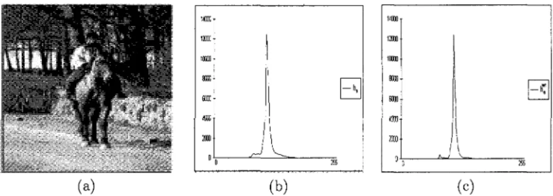
In some images, edge pixels can cause overlappings or noises between the color histogram populations. A con-sequence of not considering edge pixels in the formula (10) is the avoidance of these overlappings or noises. The following figure gives an example of the separation between two modes of a histogram.
van \m •m tan 6CC0 too mo
1
J
|l
0 2SS (b)Figure 1: Separation between two histogram modes: a) Color image, b) The a component histogram before edge region elimination and c) The a component weighted histogram.
2.5 Edge regions
For these regions the weight Wfce(i, j) in the formula (3) is given by W%(i,j) = X]v,+°o[( ><max{i, j) Um a x( i , j),
for each k = a,b. Therefore, the weighted color histograms are the multispectral gradient module weighted histograms which are given by
M-1N-1
hUc) = ^2 ] L 5(Ik(i'J) - c) X]r,,+oo[( >>max(hj) )*>max(i,j),
i = 0 j=0
(11)
for each c € {0, ...,255} and k = a,b. Thanks to the term X]?7,+oo[( ^max{i,j) ), the weighted histogram h%(c) takes into account the high values of the multispectral gradient modules. Thus, it provides information about the overall contrast in chrominances.
According to the formula (11), two color images having same colors and object shapes, but different object sizes, can have different multispectral gradient module weighted histograms. To overcome this drawback, we can consider the means of the multispectral gradient modules. In fact, the means represent the gradient module global values of a chrominance. For each chrominance, the multispectral gradient module mean histogram is given by
he/A
for each c € {0,...,255} and k = a,b, (12)
m =
#
(c)
NP,k{c)
where NPtk(c) is the number of the edge region pixels and is defined as
M-1N-1 , v
NP,k(c) = J ! 5 Z ^ (/ f c( * ' j ) -c) X ] » 7 , + o o [ f ^max(i,j)J,
i—n ->—n \ /
(13)
for k = a,b.
3 Wavelet decomposition, compression and quantization of an
his-togram
3.1 Histogram and multiresolution analysis
An histogram is a (ID) image or signal supported by 2J pixels ( J G N) and represented by a sequence of coef-ficients {if} -_0 • In order to analyse the histogram we use the Daubechies-8 wavelets. In fact, Daubechies-8
wavelets are continuous functions which can analyse continuous (ID) signals more efficiently. Also, Daubechies-8 wavelets are a good compromise between computational time and performances, since they have eight coeffi-cient overlapping filters. Furthermore, they have four vanishing moments which produce as marked a contrast in wavelet coefficient sizes between smooth and non-smooth sections of the (ID) signal.
The Daubechies-8 scaling function is compactly supported by the interval [0, 7] and its values can be calcu-lated thanks to a given initial value and to a recurrence relation which is given by
t = 7
0 ( x ) = ^ M ( 2 x - i ) , (14)
i=0
where (h0 = -0.014, hi = 0.046, h2 = 0.043, h3 = -0.264, h4 = -0.039, h5 = 0.890, h6 = 1.009, h7 = 0.325) is
the lowpass filter.
The Daubechies-8 scaling function <f> serves as the basic building block for its associated Daubechies-8 wavelet function, denoted by ip, and defined by the following recursion
i=l
1>(x) = E (-l)%-itf(2z - i). (15)
t = - 6
In order to ensure that </> and i/> are compactly supported by the same interval [0,7] and are equal zero out-side it, we shift the Daubechies-8 wavelet function ip from x to x — 3. The scaled, translated and normalized versions of <\> and the shifted version of ip are denoted by (j>\(x) = V2~(J~^(f>(2~^J^^x — i) and i>\{x — 3) =
For the finest resolution level, we introduce a vector space VJ which is the set of all possible linear combi-nations of the Daubechies-8 scaling function shifted versions. With implicit periodicity considerations, we can write
VJ=IAn{4>i : i = 0 , . . . , 2J- l } . (16)
By supposing that the (ID) signal I £VJ,we can approximate it as follows
2J- 1
I(x) ~ £ If fa - i). (17)
i=0
We define the vector subspace W3^1 = Lin{ij)f~x : i — 0,...,2J~1 - 1} to be the orthogonal complement of
yj-l i n yJ_ Explicitly
VJ = VJ-1@WJ-1. (18)
The Daubechies-8 wavelet transform decomposes the 2J pixel (ID) signal into its components for J different
scales. It consists of passing successively from the space VJ to the space V°, while generating through this decomposition the spaces {W^}J~Q. So we obtain
J - I
VJ = V°®($)Wk. (19)
fc=o
Consequently, we can rewrite the 2J pixel (ID) signal in the Daubechies-8 basis as follows
j-\V-\
I{x) ~ i^lix) + E E
!ittfr -
3)> (
2 0)
j=0 fc=0
where IQ is the overall average of the (ID) signal, called the scaling factor. The Daubechies-8 wavelets transform decomposes an histogram having 256 pixels into its components for 8 different scales. Consequently, the smooth components and the detailed components of the histogram are readily seperated. The resulted scaling factor represents the average of the histogram Y-coordinate magnitudes. Therefore, the scaling factor of a Daubechies-8 wavelet decomposed histogram of a LAB color image component, represents the average of the overall intensity of this latter.
3.2 Signal compression a n d quantization
The compression is carried out on the number of the retained coefficients representing the decomposed (ID) image. The wavelet coefficients represent the local intensity variations in the image. Their magnitudes represent the importance of the variations, but their signs express the type of these variations. If we keep only the coefficients with largest magnitudes, we can obtain a good approximation of the decomposed image. Only the absolute values of the wavelet coefficients are taken into account during the compression. In the compression method we rewrite the decomposed (ID) image (20) as follows
2J- 1
I(x) * I[0]4>°0(x) + ^ / [ ^ ( x ) , (21)
i = l
where I[i] = Pk and iii(x) = ip3k{x — 3) for (i = 2j + k, k = 0, ...,2j — \,j = 0,..., J - 1). By summing these coefficients in order of decreasing magnitude and by using a permutation a, we obtain
2J- 1
I{x) ~ 7[0]$(x) + Y, lHi)]ua{i)(x), (22)
where
! I\cr(ii)} \>\ I[(T(i2)} | for all 0 < h < i2. (23)
Consequently, when we keep the m largest coefficients, we obtain an approximation Ic(x) representing the
compressed version of the decomposed (ID) image I{x), defined by
2J- 1
I
c(x) ~ i[0]$(a:) + J2 ~
IC[^i{x), (24)
j = i
where
fcr.-i _ / I[*\ i f l <o- 1(i)<m, / „
-This approximation introduces an error called the L2-error given by
i-
r
2 - 1
E (
J>«])
2 (26)The retained coefficients after the compression, have the largest magnitudes and the most relevant data in the decomposed (ID) image. However, the storage of these coefficients requires a large space. For this reason, we
use a quantization of our (ID) images which reduces the storage space. Every significant non-zero coefficient is quantified to just two levels: + 1 represents the largest positive coefficients, and —1 represents the largest negative coefficients. Therefore, the quantified version Iq of the compressed (ID) image Ic is given by
2J- 1
/«(*) ~ J[0]$(s) + £ 3[t]fi,(a:), (27)
where C + 1 if P[i] > 0, Icq\i] = < 0 if Jc[i] = 0 , i = 1,..., 2J - 1. (28) [ - 1 if Ic{{\ < 0.4 The metric and t h e querying algorithm
4.1 The metric or pseudo-metric
In the last section, we showed that the compression gives us a good approximation of the Daubechies-8 decom-posed (ID) image and the quantization reduces its storage space. According to [5], if we consider only the signs of the retained and quantified coefficients after the compression in the querying, we can reduce the comparison algorithm execution time.
Let us consider Q and T as the query and the target (ID) images, respectively. The (ID) version of the metric, proposed by [5] is obtained from the following expression
2J- 1
| | Q , T | | = a ; o | Q [ 0 ] - r [ 0 ] | + £ w«|QS[»]-T,c[i]|, (29) »=i
where o>$ are the metric weights, Q[0] and T[0] are the scaling function coefficients of the ID images Q and T, and Qg[i] and Tj:[i] represent the i-th decomposed, compressed and quantified coefficients of these latters. Since the possible values of a coefficient are + 1 or — 1, the term
| $ [ i ] - T ,c[ t ] | e j o , l , 2 } . (30)
In the following case
Q and T preserved their coefficients at the i-th position despite the decomposition and compression, but the
two coefficient signs don't match. They have opposite variations. With respect to the distance between two different images, two opposite variations having the same positions don't represent more proximity than when one of them is equal to zero after the compression. Also, since we assume the vast majority of database images not to match to the query (ID) well at all, the number of mismatches is larger than the number of matches. That's why we write our metric as follows
|| Q,T ||= W0|Q[0] -f[0}\ + £ W i f e ] 7 ^ [ A (32)
where
In order to make the metric faster, we only consider terms in which the query has a non-zero wavelet coefficient. A disadvantage of this approach is that we technically disqualify our metric from being a metric because of its asymmetry. Because of this modification our metric becomes
|| Q,T ||= o;0|Q[0]-f'[0]|+ ] T wA Qg[i\ * fcq\i] J. (34)
To compute the metric over a database of (ID) images, it's generally quicker to count the number of matching coefficients of Qq and Tq than mismatching coefficients. For this reason, we rewrite
]T
Wife]^T£[i]) = J2 " i - E " i f e ] = ^ ] ) > (35)
whereSo our metric becomes
Q
)T||=
Wo|0[o]-r[o]|+ £ m- E «i(Q
cS =
fcq^)- (
37)
Since the sum of the terms Wi is independant of every target T9C, we can discard it. Consequently, we obtain
|| Q,T ||= u>
0\Q[o]-f[o}\- Yl ^ f e ] =
f 9 cw ) - (
38)
To simplify, we suppose that the weights associated to the coefficients belonging to the same scale, are identical. Thus, we group the weights according to the resolution levels, by using a simple bucketing function bin{) such as bin(i) represents the floor of log2(i) for i € {1,..., 2J — 1}
bin(i) = [log2{i)\ with i = 1,..., 2J - 1. (39)
Consequently, we use a set of weights wo and {WJ},~Q and define the UJQ and uVs by
\ u>i = Wj for J G 2 ^ + {0,..., 2j - 1} and j = 0,..., J - l ( j — bin(i)),
where J is the maximum number of resolution levels. Finally, it suffices to compute the expression
|| Q,T ||= «)o|g[0]-:f[0]|- Yl Wbin(i)(Q
cg[i\^T
gc[i\). (40)
4.2 One-dimensional image querying algorithm
In order to optimize the metric computation process, we introduce two arrays called search arrays. Let 6+
for the coefficients quantified to + 1 and 0 _ for those which are quantified to —1. Each array contains 2J — 1 elements and each element contains a list. For example, the element 9+[i] points on the list of all the database (ID) images having a large positive wavelet coefficient at the i-th position, after compression. With the same way, the element 0_[i] points on the list of all the database (ID) images having a large negative wavelet coefficient at the i-th position. Thanks to these arrays and to the compression, during the querying process we have just to go through the m lists associated to the query m retained coefficients instead of 2J — 1 coefficients. After the creation of the search arrays and weights WQ and {wi}^ computation, the retrieval procedure of a query Q in the database of (ID) images Tfc (k = 1,..., |.DJB|), where |.D.B| denotes the database size, is defined as follows
Q <— FastDaubechiesWaveletsDecomposition(Q)
Initialize Score[k] = 0, for each k e {1,..., |Z)Z?|} For each k e {1,..., \DB\) do
Score[position of Tk in the (DB)] = w0 * |Q[0] - Tfc[0]|
end for
Qc <— Compress(Q,m)
Qcq <- Quantify(Qc)
For each Q£[i] ^ 0 do If Q£[i] > 0 t h e n
List *-@+[i] Else
List <- 6_[z] End if
for each 2 of List do
Score [position of I in the (DB)] = S'corelposition of I in the (DB)] - Wun(i) End for
End for Return Score
End procedure
This procedure returns an array Score such that Score[k] =|| Q,Tfe || for each k e {1,..., |JDB|}. The array
Score elements which are the similarity degrees between the query Q and the database (ID) images Tk {k e
{1,..., |D-B|}), can be negative or positive. The most negative similarity degree corresponds to the closest target to the query Q.
4.3 Weights a d j u s t m e n t a n d logistic regression
The logistic regression is one of the most popular data mining tools. In content-based image retrieval field logistic regression was used to model the relevance feedback [8]. In our application, the logistic regression can be used to tune the weights of our metric. A weight w^ represents the corresponding relative importance of a query fc-th resolution level coefficients, retained after the compression, to a target coefficients belonging to the same resolution level and having the same positions and signs. Note that if we set the weights WQ and
to different resolution levels have the same corresponding relative importance to the query different resolution level coefficients. We devide our target set into two classes: a matching class and a mismatching class. Each class contains a set of observations extracted from the database. The logistic regression method introduces a binary target variable and a set of explanatory variables to represent the class of a given observation. Specifically
Y : Target variable
yr — 1 case of mismatch with the target T = 0 case of match with the target T tr_ = {io,T,to,r, —,tj-i,T) '• Explanatory variables,
where io,T is the absolute value of the difference between the scaling factors of the query and the target T, {£fc,r}fc=o a r e the numbers of mismatches between the fc-th resolution level coefficients of the query and the
target T, J is the maximum number of the resolution levels and JJT is the binary target variable, it's either 0 or 1, depending on whether or not the query and the target T are intended to match. We assume a posterior probability of the mismatching with the target T, given the explanatory variables is p?, i.e., pr = P(yT\tr)- In our logistic regression model we assume that posterior probability is given by
PT = P\VT = l\tr_) = F(w0i0,T + 5^Wfc*fc,r)> (4 1) fc=0 and J - I PT = ! ~PT = P[yr =0\tr) = F{-w0i0)T - ^ k i v ) , (42) ^ ' fc=o
where WQ and {wk}JkZl are the weights to compute and
*"(*) = TT*-
(43)In order to tune the weights, we perform a maximum likelihood estimation. The likelihood function measures the likelihood that different tr_ have given rise to the observed yr- Provided observed target variables have independent Bernoulli distribution with the probabilities PT for each target T, the form of the likelihood is
given by n L(w0,w0,...,Wj^) = \[pyTT{l-PT)l-yT (44) T=l na n i = Y[(1-PT)Y[PT, (45) T = l T = l
where n is the number of all observations and UQ and n\ are the numbers of cases with target variable value 0 and 1, respectively. We want to choose VOQ and {wk}kZ,Q so as to maximize the natural logarithm of the above likelihood. This can be done by using the software SAS 6.12 or the Fisher-scoring algorithm. The training is an important step in the logistic regression method to extract the observations from the database.
4.4 Training (for t h e logistic regression m e t h o d )
Let us consider a color image database which consists of several color image sets such that each set contains color images which are perceptually close to each other in terms of object shapes and colors. In order to compute the metric weights wl0 and {wlk}rk=0 (I e {1, ...,N}) by the logistic regression, we have to create the matching classes (ylT = 0) (I € {1,...,N}) and the mismatching classes (ylT — 1) (I e {l,...,iV}). To create a single matching class (ylT = 0), we draw all possible pairs of histograms or feature vectors representing color images belonging to the same database color image sets, and for each pair we compute the values of il0 T and {tlk T}kZ0 • Similarly, to create a single mismatching class (ylT = 1), we draw all possible pairs of histograms or feature vectors representing color images belonging to different database color image sets, and then for each pair we compute the values of i^ T and {tlk T
}fc=o-5 Color image retrieval method
The querying method is in two phases. The first phase is a pretreatment phase done once for the entire database containing \DB\ color images. The second phase is the querying phase.
5.1 Preprocessing (of the LAB color image database)
We detail the preprocessing phase done once for all the database color images before the querying in a general
case by the following steps.
2. Compute the N feature histograms Tu (I G {l,...,iV}) for each i-th LAB color image of the database,
where i e {1,..., \DB\}.
3. The feature histograms representing the database color images are Daubechies-8 wavelets decomposed, compressed to m coefficients each and quantified.
4. Organize the decomposed, compressed and quantified feature vectors into search arrays 0 + and 6;_
(Z = l,...,iV).
5. Adjustment of the metric weights wl0 and {wlk}7k=0 for each set of feature histograms Tu (i — 1,..., \DB\) representing the database color images, where I € {1,..., N}.
5.2 The querying algorithm
We detail the querying algorithm in a general case by the following steps.
1. Given query LAB color image. We denote the feature vectors representing the query image by Qi (I = l,...,iV).
2. The feature vectors representing the query image are Daubechies-8 wavelets decomposed, compressed to
m coefficients each and quantified.
3. The similarity degrees between Qi (Z = 1,.,.,N) and the database color image feature histograms Tu (Z = 1, ...,JV) (i = 1,..., \DB\) are represented by the arrays Scorei (Z = l,...,iV) such that Scorei[i] =||
Qi,Tu || for each i 6 {1,..., |J9B|}. These arrays are returned by the procedures Retrieval(Q;, m, 6; +,
@i.) (I = 1,..., N), respectively.
4. The similarity degrees between the query color image and the database color images are represented by a resulted array TotalScore, such as, TotalScore[i] = J2i=iliScarei[i] for each % e {1,..., |-D-B|}, where {7(}i^i a r e weightfactors used to fine-tune the influence of each individual feature.
5. Organize the database color images in order of increasing resulted similarity degrees of the array TotalScore. The most negative resulted similarity degrees correspond to the closest target images to the query image. Finally, return to the user the closest target color images to the query color image and whose number is denoted by RI and chosen by the user.
5.3 The querying method dataflow diagram
For simplicity, we describe t h e querying m e t h o d steps by t h e following diagram.
Preprocessing
Querying
[Extraction of N feature histograms from each database LAB color image.
Extracted feature histograms are Daubechies-8 wavelets, decomposed
compressed and quantified.
I
Construction of'the search arrays for each set of feature histograms.
T
Adjustment of the metric weights, for each set of feature histograms.
Extraction of N feature histograms from the LfiB query color image.
I
The query color image N feature histograms are Daubechies-8 wavelet*
decomposed, compressed and
quantified.
T
The strnilarity degrees .between the
query color1 image N feature histograms
and the database color image feature
histograms are computed using the procedure Retrieve! and then are
represented by the arrays Scorsg (1 = 1., ,N).
T
The similarity degrees between the query eotor image and the database color images are represented by the resulted array TotafScore, such us,
A'
TotalScortfi] = y y, Scorej[/]
1=1
for each ; ' e { l , \D3\\
T
The most negative resulted similarity degrees correspond to the closest target images to the query image.
6 Experimental results and evaluation
In this section we perform some experiments to validate and evaluate our querying method in a database of
\DB\ = 10000 animal, landscape, art, bridge and building LAB color images. It consists of several color image
sets such that each set contains color images which are perceptually close to each other in terms of object shapes and colors.
The first evaluation will be based on a comparison between the querying after using classical color histograms
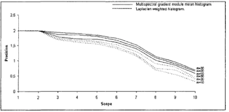
h,L, ha and h(, given by (1), and the querying after using hi, h\, h^, hea and h^ given by (1), (9) and (12), respectively, to represent the database color images. The second evaluation will be based on a comparison between the querying results when the metric weights are equal to 1 and the querying results when the metric weights are computed by the logistic regression. In this evaluation each database color image is represented by its hi,, h%, 11%, hi and hi. The third evaluation will be based on a comparison between the querying after using
hi, fto, h% given by (1) and (9), respectively, and the laplacian weighted histograms proposed by [6], and the
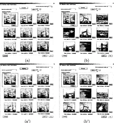
querying after using hi, h%, h%, hi and hi, to represent the database color images. In the fourth evaluation we will show the importance of considering the metric term ifto|<2[0] — T[0]\ or the scaling factors in the querying. Finally, the fifth evaluation is carried out to show the improvement of the querying results thanks to the query color image h\ and hi transformation used to make the querying invariant to the color intensities of the query color image.
Generally, to carry out an evaluation in the image retrieval field, two principal issues are required: the ac-quisition of ground truth and the definition of performance criteria. For ground truth, we introduce human observations. In fact, two external persons participate in the all below evaluations. Concerning performance criteria, we represent each evaluation results by the precision-scope curve Pr = f(RI), where the scope RI is the number of images returned to the user. In each querying performed in an evaluation experiment, each human subject is asked to give a goodness score to each retrieved image. The goodness scores are 2 if the retrieved image is almost similar to the query, 1 if the retrieved image is fairly similar to the query and 0 if there is no similarity between the retrieved image and the query. Consequently, we can compute the precision as follows:
Pr = the sum of goodness scores for retrieved images/i?I. Therefore, the curve Pr = f(RI) gives the precision
for different values of RI which lie between 1 and 10 in our evaluation experiments. When the human subjects perform different queryings in the same evaluation experiment, we compute an average precision for each value
of RI, and then we construct the precision-scope curve.
The following experiments will be carried out to extract the curve Pr = f(RI) for each evaluation men-tioned above.
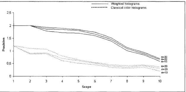
F i r s t e x p e r i m e n t
This experiment is carried out to show the advantage of using our weighted histograms instead of classical color histograms to represent the query color image before the querying. Each human subject is asked to formulate a query from the database and to execute a querying using N = 3 feature histograms which are fiL, ha and hb given by (1), to represent the query color image, while computing the metric weights by the logistic regression and keeping the weightfactors {7/}?=i equal to 1, and to give a goodness score to each retrieved image, then to reformulate a query from the database and to execute a querying using N — 5 feature histograms which are
h>L, h-a, h1^, hea and h\, to represent the query color image, while computing the metric weights by the logistic regression and keeping the weightfactors {7;}f=1 equal to \ and 74 and 75 equal to 1 to give more importance
to the edge region features, and to give a goodness score to each retrieved image. Each querying is repeated twenty times by choosing a new query from the database each time. We repeat this experiment for different orders of compression m e {30,20,10}. The resulted precision-scope curves are
2,5 -I 2 • c 1,5-.£ ™ £ 1 • 0 , 5 -1 2 • " • ' • ' ' " • ' • " ^ v : : : -3 4 5 6 Scope 7 8 9 SE E E E E 10
Figure 3: Evaluation: precision-scope curves for retrieval when the database LAB color images are represented by /i£, ha and hb each, and when the database LAB color images are represented by tiL, h%, hft, hea and h\ each, for the compression orders m e {30,20,10}.
separation between the modes of the color histograms representing the database LAB color images and to the use of the multispectral gradient module mean histogram to consider the database color image edge regions in the querying. We choose the same query for the three examples. For each example the query is located at the top-left of the dialog box.
;S;M;KW.«W*VAM i • . - . , . * Bmwn—H—WKHKKK0smmmmsmMn
(a) (b)
E 3 ! 'SsSs Q 3 : SS3 H ' 3
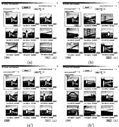
(a') (b') Figure 4: Comparison (m = 30): a) first 7 color images retrieved after being represented by their hi, ha and
hb, b) second 7 color images retrieved after being represented by their hi, ha and hi,, a') first 7 color images retrieved after being represented by their hL, ft£, /i£, hea and hi and b') second 7 color images retrieved after being represented by their hi, h%, h%, h% and h\.
QgggU?
m
- j
m
-
m
- [™!*^-^i
rmmm w
.SB
(a) (b)
mid &$ M£ mti* &:^
m
«*!
JSP LsJ
(a') (b')
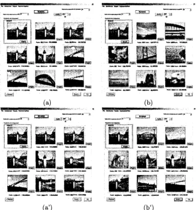
Figure 5: Comparison (m = 20): a) first 7 color images retrieved after being represented by their hi, ha and
hb, b) second 7 color images retrieved after being represented by their hi, ha and hb, a') first 7 color images retrieved after being represented by their hi, /i£, h\, hea and h\ and b') second 7 color images retrieved after being represented by their hi, h\, h\, hea and h\.
. _ . £ S B J ~ — WfVSWim If j f>"> "-T--TT - " • ! (a) TWltt—'
at^ ee
1
^
i ^
(a') ruaair K 9 JSB.J — — « M i f f » » » sgg D O (b) £5BL 4 •1 P F " » . (b-) SBFigure 6: Comparison (m = 10): a) first 7 color images retrieved after being represented by their hi, ha and
fit,, b) second 7 color images retrieved after being represented by their hL, ha and ht,, a') first 7 color images retrieved after being represented by their hi, ftj, ft£, ft® and ft| and b') second 7 color images retrieved after being represented by their ft/,, ftjj, ftj, ft£ and ftjj.
Second e x p e r i m e n t
This experiment is carried out to show how the weights computed by the logistic regression can optimize our querying results. Each database color image is represented by UL, h*l, h%, hea and h^ Each human subject is asked to formulate a query from the database and to execute a querying, using weights computed by the logistic regression, and to give a goodness score to each retrieved image, then to reformulate a query from the database and to execute the querying, using weights equal to 1, and to give a goodness score to each retrieved image. Each querying is repeated twenty times by choosing a new query from the database each time. We repeat this experiment for different orders of compression m e {30,20,10} and we keep the weightfactors {7/}f=1 equal to \ and 74 and 75 equal to 1 to give more importance to the edge region features. The following table contains
the weights computed by the logistic regression, for order m = 30 of the compression.
hL(l = 1) K(l = 2) KQ = 3) >£(* = 4) K(i = 5) w>o 3.31 3.59 5.14 5.78 5.63 wl0 7.23 4.65 8.29 5.67 8.08 w[ 5.34 6.28 3.51 8.52 6.18 wl2 6.85 8.26 4.40 7.04 9.37 wl3 8.51 4.38 8.59 6.85 9.47 U>4 8.37 6.37 5.90 8.01 5.05 wl5 6.24 7.21 8.72 7.09 7.57 wl6 7.25 10.41 7.83 6.82 8.43 wl7 10.14 3.91 6.93 6.62 7.94
Table 1: Weights computed by the logistic regression for TO = 30.
The resulted precision-scope curves for each compression order are
2,5 -,
1,5
o. 1
0,5 H
Weights computed by the logistic regression. Weights equal to 1.
5 6 Scope
10
Figure 7: Evaluation: precision-scope curves for retrieval using weights equal to 1 and weights computed by the logistic regression, for the compression orders m 6 {30,20,10}.
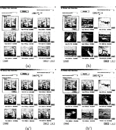
The following three Figures give three examples of the improvements of our querying results when we use weights computed by the logistic regression instead of weights equal to 1, to tune the metric. We choose the same query for the three examples. For each example the query is located at the top-left of the dialog box.
-—""•' i«a«n;i La* i h'£ H Lfc^fc! ' Sf4 1 oaa ua a s raa (a) (b) ESSep i * f ^ i.. rs~i ,™„„u. \**\\ f£.S W " " (a')
*1 I iL '
(b') E»a i±iFigure 8: Comparison (m = 30): a) first 7 color images retrieved after using weights equal to 1, b) second 7 color images retrieved after using weights equal to 1, a') first 7 color images retrieved after using weights computed by the logistic regression and b') second 7 color images retrieved after using weights computed by the logistic regression.
l i i U I I lt&\^ lv 'U>1 I , Si * s i _ j asa iaa (a)
ugJ
^
(a') £53 S 3 •;*^##*l ' m' (b) [~Ti«irTit
J S S J "«-<r
,*H*f*. Bag.Pi
(b')Figure 9: Comparison (m = 20): a) first 7 color images retrieved after using weights equal to 1, b) second 7 color images retrieved after using weights equal to 1, a') first 7 color images retrieved after using weights computed by the logistic regression and b') second 7 color images retrieved after using weights computed by the logistic regression.
L _ cssj. > X
o yfefi
r (a) •ii«!,r|; fc •arc: I'1m
£33 LSJ (b) , S l .^ y
' B i (a') {S3 UU (b')Figure 10: Comparison (m = 10): a) first 7 color images retrieved after using weights equal to 1, b) second 7 color images retrieved after using weights equal to 1, a') first 7 color images retrieved after using weights computed by the logistic regression and b') second 7 color images retrieved after using weights computed by the logistic regression.