Développement d'un modèle géochimique, numérique et transposable pour la prédiction de l'acidifications des eaux de surface = Development of a transportable numerical geochemical model to predict the acidification of surface waters.

Record Number:

Author, Monographic: Jones, H. G.//Roberge, J.//Laberge, C.//Sochanski, W.//Stein, J. Author Role:

Title, Monographic: Développement d'un modèle géochimique, numérique et transposable pour la prédiction de l'acidification des eaux de surface - Partie 1: chap. I-III Development of a transportable numerical geochemical model to predict the acidification of surface waters - First part: chap. I-III

Translated Title: Reprint Status: Edition:

Author, Subsidiary: Author Role:

Place of Publication: Québec Publisher Name: INRS-Eau Date of Publication: 1990

Original Publication Date: Février 1990 Volume Identification:

Extent of Work: 131

Packaging Method: pages Series Editor:

Series Editor Role:

Series Title: INRS-Eau, Rapport de recherche Series Volume ID: 284

Location/URL:

ISBN: 2-89146-281-5

Notes: Rapport annuel 1989-1990

Abstract: 20.00$

Call Number: R000284 Keywords: rapport/ ok/ dl

Development of a transportable numerical geochemical

model to predict the acidification of surface waters

Première partie: Chapitres 1-111

First part: Chapter 1-111

H.G. Jones, 1NRS-Eau J. Roberge, 1NRS-Eau C. Laberge, 1NRS-Eau

w.

Sochanski, 1NRS-Eau J. Stein, Université Laval

1NRS-Eau, rapport scientifique No 284

TABLE DES MATIERES

RESUME

1. Article: A statistical approach to field measurements of the chemical evolution of cold « DOC) snow cover (Une approche statistique pour la mesure de l'évolution chimique du couvert

Page

de neige en période froide « DOC)) ... ... ... ... 1-1

II. Article: SNOQUAL, a model for the simulation of meltwater

quantity and quality in boreal fore st catchments; a study of the model variants for the chemistry of snow meltwaters (SNOQUAL, un modèle pour simuler la quantité et la qualité des eaux de fonte dans des bassins de la forêt boréale; une étude de trois versions

du modèle pour la chimie des eaux de fonte) .. ... ... 11-1

III. Article: The discrimination of the origins of sub-ice acidic waters in a small lake during the apring runoff. (L'identifica-tion des origines des eaux acidifiées sous le couvert de glace d'un petit lac pendant la fonte printanière) ... .

APPENDICE

Ce rapport comprend 4 parties. Les trois premiers chapitres concernent les activités de recherche et développement du modèle de fonte du couvert de neige "SNOQUAL" telles que définis dans le contrat de recherche "Development of a transportable numerical geochemical model to predict the acidification of surface waters". Chaque chapitre est précédé par un résumé en français. La quatrième partie, l'annexe, comprend les données de fonte 1988 utilisées dans ces travaux.

Le premier chapitre liA statistical approach to field measurements of the chemical evolution of cold

«

DOC) snowcover" est identique à l'article du même nom accepté pour publication dans la revue "Environmental Monitoring and Assessment". Cette publication encadre les travaux de recherche orientés vers la prédiction des conditions initiales du couvert de neige avant la fonte. L'article, en effet, décrit la méthodologie statistique que nous avons employé sur le terrain pour évaluer l'évolution quantitative de la concentration de S04 dans le couvert en période froide. Les résultats nous permettront d'évaluer d'une façon plus précise les pertes ou les gains des anions d'acidité forte pendant la période d'accumulation du couvert qui précède la fonte printanière.

Le deuxième chapitre représente une publication qui a été présentée au "Chapman Conference: Hydrogeochemical Responses of Forested _{Catchments " , 18-24} septembre, Bar Harbor, Maine. Cette publication sera, de plus, soumise au "Water Resources Research" en 1990. Les travaux décrits dans cette publication Si i nsp i rent du mandat de l'INRS-Eau dl amé li orer l a performance du modèle de fonte SNOQUAL1 en y introduisant des paramètres de compensation pour les écarts entre la composition des eaux de fonte produite par le modèle et celle observée

"in situ". Par la suite, le modèle tel qu'amélioré aurait dû permettre de mieux simuler la composition des eaux de fonte, et ceci, pour que nous puissions établir des valeurs probablistiques pour k, le coefficient de lessivage des anions d'acidité forte du couvert de neige. La publication met en évidence les travaux de développement du modèle de fonte en décrivant deux modèles (SNOQUALR et SNOQUALD) dont les structures reflètent des processus physico-chimiques et

microbiologiques dans le couvert. Ces processus sont: i) 1 a présence dl une

certaine quantité des ions qui résident à 11 intérieur des grains de neige et

qui ne subissent que très peu de lessivage, et 2) du matériel autre que celui compris sur, et dans, les grains de neige au commencement de la fonte. Ce

matériel additionnel contribue pendant la fonte à la composition finale des

eaux par les processus de dépôts secs, le lessivage lent des matières organiques et l'activité microbiologique. De ces travaux, il s'avère que le

modèle SNOQUALR qui intègre un paramètre relié à la quantité des ions résiduels

dans la neige est présentement le modèle le plus performant. Suite au

développement du modèle SNOQUALR nous avons déterminé une valeur moyenne pour le coefficient de lessivage des ions d'acidité forte. Le modèle a ensuite permis la simulation de la composition physico-chimique (et le pH) des eaux de fonte selon des conditions hypothétiques d'une réduction de 30% et 50%, et une augmentation de 30% dans les émissions de SO, dans l'est de 1 'Amérique du Nord. Ces travaux de simulation ont démontré que le processus de lessivage est tellement dominant dans le contrôle de la composition des eaux de fonte que la réduction d'émissions (et, par surcroit, la réduction de concentration d'anions d'acidité forte dans la neige) ne résultera pas en une diminuation appréciable du pH des eaux de fonte.

l'essentie1 a été accepté pour présentation au Symposium sur IIEpisodic chemistry of streams and 1akes ll de 11_{American Geophysical Union, du 4 au 9}

décembre 1990, San Franci seo et IIThe E i ghth Internat iona 1 Northern Research Basin Symposium and Workshop, Abisko, Sweden, 26-30 Mars 1990. _{L' artic1e sera}

soumis incessamment à IIWater Resources Research ll pour fins de publication. Cet article démontre la chronologie de l 1 acheminement des eaux de fonte de diverses

sources sous le couvert de glace du Lac Laf1amme pendant la fonte printanière. Ces travaux nous renseignent, d'une façon plus explicite, sur 11 importance relative des eaux de diverses origines et nous permettront de mieux prédire la composition chimique de l'écoulement printanier dans le bassin. Il faudrait noter que les écoulements acides au Lac Laf1amme se reproduisent sous la glace. La disparition du couvert, en effet, résulte en une réduction considérable de 11

acidité des eaux de 11

épilimnion par la remonté des eaux d'hypolimnion due à

11

inf1uence du vent.

Ce rapport comprend, de plus, une annexe dont 1 e contenu est const itué de données physico-chimiques de la neige, des eaux de fonte, des eaux de ruissellement et des eaux lacustres du Lac Laf1amme, printemps 1988.

CHAPITRE 1 CHAPTER 1

A statistical approach to field measurements of the chemical evolution of cold «

DOC)

snow cover (Une approche statistique pour la mesure de l'évolution chimique du couvert de neige en période froide «

DOC)

Claude Laberge*

INRS-Eau, 2800 Einstein, Sainte-Foy (Québec), G1X 4N8

H. Gerald Jones

INRS-Eau, 2700 Einstein, Sainte-Foy (Québec), G1V 4C7

1-2

Résumé

L'application de deux méthodes statistiques connues à des expenences sur l'évolution de la composition physico chimique du couvert de neige en période froide

«

OOC), a permis de relier leurs qualités statistiques aux coûts qu'elles engendrent

sur le terrain. Les méthodes utilisées étaient la régression (expérience avec une ob-servation par jour d'échantillonnage pendant une longue période froide) et l'ANOVA (expérience avec plusieurs réplicats par jour d'échantillonnage pendant une période froide restreinte). Les puissances relatives théoriques des deux méthodes permet-tent de déterminer l'amplitude des changements chimiques que l'on peut détecter. L'utilisation d'estimateurs de la variance permet finalement d'estimer l'amplitude absolue (en peq [-1 ) que l'on peut détecter.

Les résultats des applications, sur l'évolution des sulfates au Lac Laflamme (Québec), montraient clairement des pertes de sulfates pour six des huit strates étudiées durant des périodes froides. Les amplitudes relatives des pertes signi-ficatives variaient entre 1% par jour et 4% par jour, cette variation dépend des concentrations initiales et des conditions météorologiques.

La comparaison des deux méthodes statistiques a démontré que pour un même nombre d'observations, la régression détecte des amplitudes absolues beaucoup plus petites que l'ANOVA, elle est donc plus puissante pour détecter des change-ments de concentrations dans la neige. Ces informations permettent de planifier les expériences futures en incluant le coût déxpériences sur le terrain ou en laboratoire.

Abstract

Two statistical methods for the analysis of data on the evolution of the

chemical composition of cold snow ( <OOC) in the field (Lac Laflamme,

Quebec) were compared. The tests used on the data were regression analysis (1 sample per sampling date over a long cold period) and ANOVA (replicate samples on a restricted number of sampling dates over shorter periods). The relative power of the tests to determine the detectable amplitude of chemical changes was derived from the theoretical power of the tests under

comparable conditions of sampling (number of observations) and from the estimated error variances of the measured data.

The results of the study on the evolution of S04 concentrations in discretely identified snow strata clearly showed that for 6 strata out of 8, significant losses of S04 did occur in snow during cold periods. The relative

amplitude of the significant losses varied between 1% day-l and 4% day-l

depending on the initial concentrations in the snow and the prevailing meteorological conditions.

The analysis of the data also demonstrated that for the same number of samples, the regression analysis is more efficient in detecting the chemical changes in snow than the alternative ANOVA method. The use of this information to plan sampling programs of cold snow under both field and laboratory conditions is discussed.

Introduction.

Snowcover is a major reservoir of atmospheric pollutants in the

hydrologie cycle of boreal ecosystems. In the past decade the acidification of surface waters in northern regions has thus resulted in an increase in the study of snow chemistry. The main emphasis has been placed on the

temporal changes in the concentrations of strong-acid anions in snow during

the cold « 0° C ) accumulation period when the water equivalent of the pack

increases and in the melt season when the phenomenon of "acid shock" due to high hydrologie flux occurs.

snow cover is the heterogeneous distribution of the chemical species in the pack (Tranter et al. 1986). Although the chemical composition of individual snowfalls may be relatively homogeneous over a catchment area

2

(lQ-lOOkm ), subsequent wind redistribution (Delmas, and Jones 1987), small melt and freeze cycles (Colbeck 1981), and local dust and forest canopy fallout (Jones, and Sochanska 1985) will provoke small-scale disparities

2

(1-100m ) in the chemical characteristics of the snow strata laid down by the original precipitation events.

To follow chemical changes in cold snow, samples of the snow cover are taken over a period of time during which the temperature of the snow and the air are helow OOC. The sampling method is destructive for the snow cover and successive samples have to be taken as close to the original point as possible. This, however, can be a cause for concern as the removal of snow from the original sampling point can influence the remaining snow in the immediate environment by modifying temperature gradients and air-snow interchange. As the sampling period evolves the spatial requirements for the collection of the samples increases. This in turn enhances the probability that the sampling "point" will cover areas of snow with different chemical characteristics. Thus any attempt to study the evolution in the chemical composition of cold snow covers due to real processes of transformation or translocation "in situ" has to take into consideration the apparent chemical changes that result from the spatial inequalities in snow quality.

To distinguish real chemical changes in snow from any apparent

changes, the sampling strategy should be based on a statistical analysis of the spatial chemical characteristics of the snow cover at the beginning of the sampling period. In the absence of weIl defined spatial characteristics valid information on real in-pack changes can, however, still be obtained even if the spatial variability is less known. This would be true in the case where the in-pack chemical processes are consistent and result in concentration changes of species in the same direction (i.e. losses or gains) over time. The detection of a trend in time is then related to real changes large enough to overcome any masking effect by the chemical heterogeneity of the snow. In previous studies on the chemical evolution of cold snowpacks (Jeffries, and Snyder 1981; Jones, and Bisson 1984; Cadle et al. 1984) the sampling methods did not give rise to sufficient data from which definite conclusions on real changes in in-pack chemistry of snow could he drawn. The

optimisation in the quality and quantity of field data from which

unambiguous results may he obtained should thus be the major priority of the sampling methodology. Field operations are expensive: by reducing the cost in the sampling program much needed funds may he diverted elsewhere.

The following article describes two experiments which were carried out to study real changes in the chemistry of cold snow in the packs at Lac Laflamme, Quebec. To avoid any mass movement of snow (wind erosion and redeposition) during the study periods discrete in-pack strata of snow were sampled. Each study had a different sampling strategy. In the first

experiment one snow sample per stratum was taken on each sampling date

over a relatively long cold period. In the second study many replicate

samples of each stratum were taken per sampling date over short cold periods. The two data sets were treated by two simple but different statistical analyses. The set from the long period was subjected to a trend detection analysis in which spatial variability is not a factor. The second set was analysed by analysis of variance (ANOVA) where the variance of

replicates on successsive sampling dates estimates the spatial variability of snow quality. The powers of the tests involved in each method are compared and the results from the two field studies are used to estimate the chemical changes that would he detectable by each method for a reasonable sam pie size.

Site characteristics and sampling methodology.

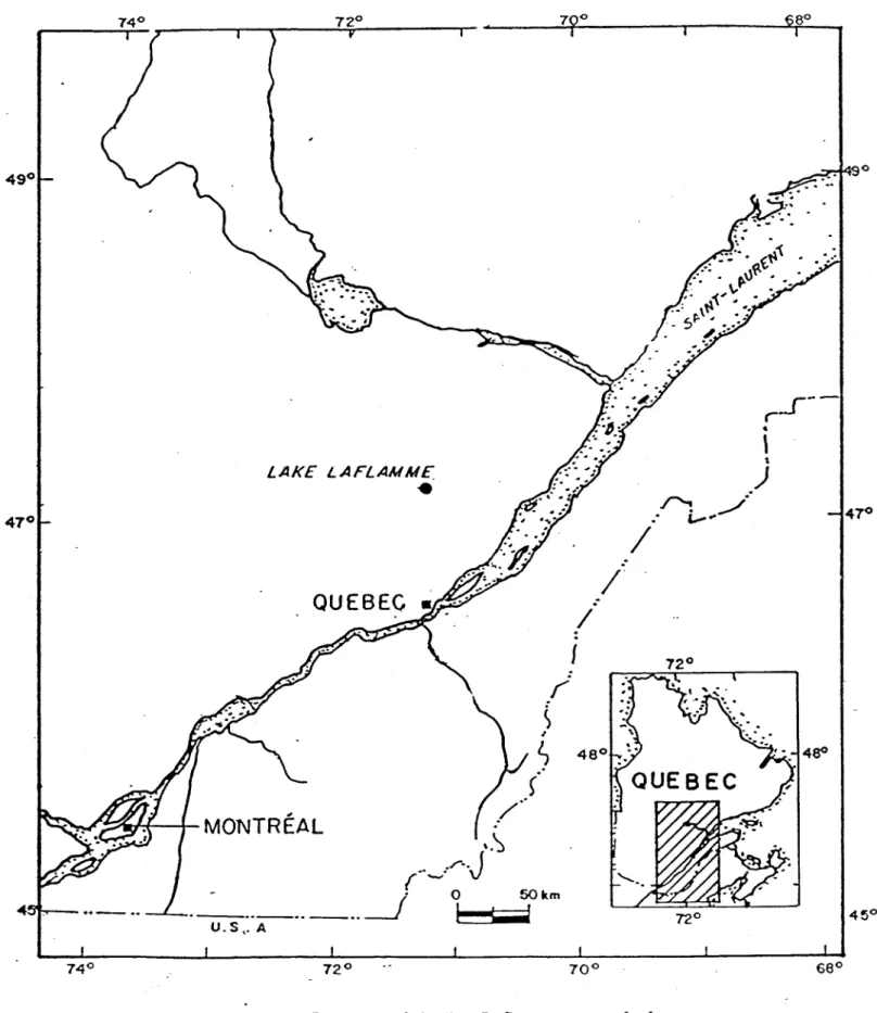
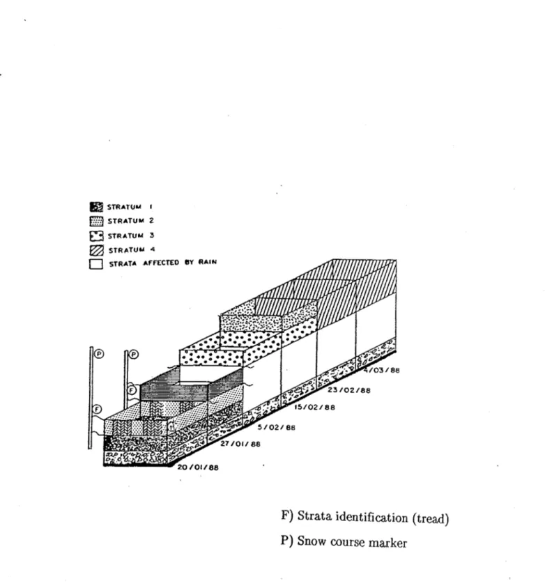
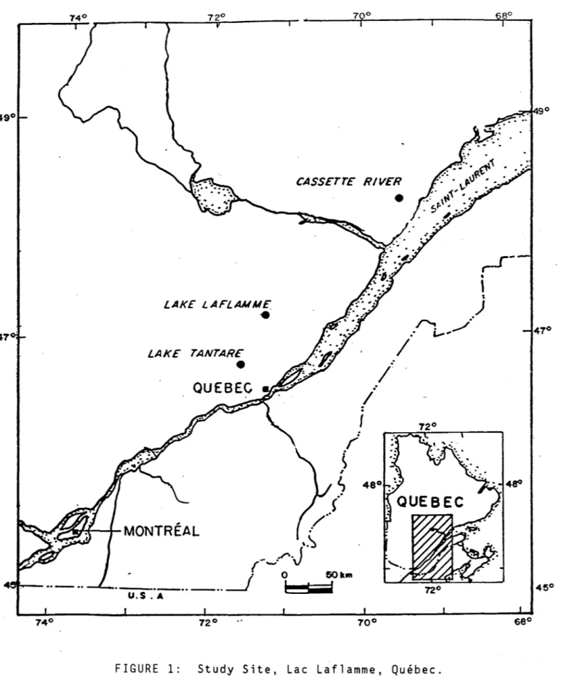
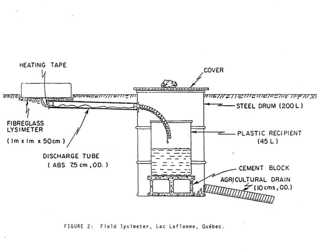
Two snow courses were laid out in the watershed of Lac Laflamme a small headwater lake (47°19' N, 71°07' W) in the Parc des laurentides, Quebec (Fig. 1). The mean annual temperature is 0.2°C ( -15°C January; 15°C, July). The total snowfall at Lac Laflamme is approximately 400 mm (Snow Water Equivalent, SWE) and the pack reaches a depth of 120-150 cm. The courses, approximately 25-30 m long and 1.5-2 m wide, were prepared before the win ter season by removing low brush and debris from open areas of the boreal forest. The length of each snow course was staked out with two parallel lines of fence posts 2m apart (Fig. 2).

The first course was sampled in 1985; four adjacent discrete strata (1,2,3,and 4), identified by means of threads, were sampled (one sample per stratum) once a week during a cold period that ran from the January 10 to

LAKE LAFLAMME.

•

tr~itttH----I~

MONTR ÉA L

./

"

,\

./ .. J

(--..,' - • 0 50 km

. _

.. _,._ .. -.-1

~l ~~! U.S,. A 7 0 "

/

.'

/

.

1

Figure L Location of the Lac Laflamme watershed.

I-6

m

STRATUM 1

[J STRATUM 2

E3

STRATUM 3

~ STRATUM 4

D

STRATA AFFt:CTEO ey RAltI

F) Strata identification (tread) P) Snow course marker

March 27. The sampling dates were January 10, 16,23 and 30, February 6,

13,20 and 27, March 7, 13,20 and 27. During the last two sampling dates,

however, sorne me1twater had began to penetrate the pack as the daytime air temperature increased in early spring.

The second snow course was sampled (5 samples per stratum) during intermittent short cold periods in 1988 when the January to March period experienced rain episodes. Rain-on-.c3now episodes displace chemical species in the pack (Jones et al. 1989) and the experiment has to be started up again with new snow strata laid down subsequent to the rain events. Four strata

(1,2,3, and 4) were sampled on two different sampling dates (Fig. 2); 8trata 1

and 2 were sampled on January 20 and 27, stratum 3 on February 5 and 15,

and stratum 4 on February 23 and March 4.

The sampling technique for 1985 and 1988 was identical; it consisted in removing a core of constant cross-.c3ectional area over the depth of each stratum by means of a small square corer of plastic. The samples were conserved at _200 C until melted for analyses. A complete analysis for major ions was carried out on each sample (Jones 1987); for purposes of discussion only the analyses for 804 are reported in this paper.

Statistica.l Approach: Background and Intercomparison between the Methods.

Trend analysis

The data from the 1985 study had to be treated by a time series analysis that would detect a trend in 804 concentrations. Of the many methods available for time series analysis those of Box and Jenkins (1976)

are the most widely used. In general, the treatment of data by the methods of these authors is restricted to modelling and prediction using ARMA models; very little attention is given to the practical determination of changes in the value of the location parameter in a definite series. Furthermore an efficient use of the Box and Jenkins methods requires a relatively large amount of data Le. at least 50 observations equidistant in time. These characteristics of the Box and Jenkins techniques make them unsuitable for the treatment of the data obtained in 1985 (10 observations over the period) and inappropriate for the majority of field experiments on

snowcover. A more fitting method for such a small data set is the detection of trends over time. Two main type of trends are generally studied. First there are monotonic trends; these are graduaI changes in time often

associated with natural phenomena (e.g. precipitation, watershed runoff). On the other hand there are step trends due to stepwise changes in system conditions; these are often the result of forces external to the system (e.g. wastewater discharges). In the case of the 1985 experiment, the nature of the changes that were to be expected for in-pack chemistry lead us to believe that tests designed to detect monotonie trends should be used.

Tests for detecting monotonie trends may be of two types. These are parametric tests and nonparametrie tests. Both types of test presuppose that successive observations are completely independent except for the possible

trend. If sorne short-term dependence exists e.g. autocorrelation or

seasonality, then the tests have to be modified to compensate for these types of dependence (Lettenmaier 1976; Hirch, and Slack 1984). Parametric tests which are best adapted to the detection of monotonic trends are those of simple linear regression over time. In the case of the analysis of the change in the concentration of any chemical species over time the regression model is:

(1)

where Ci is the concentration of the chemical at time th Co is the original

concentration, /:). is the slope of the regression, ei is a random error

component. The values of ei are assumed to be independent and identically

distributed N(O,u2). Under these conditions the estimates for the slope of the

regression and for its standard deviation indieate the significance and the

amplitude of the trend. The null hypothesis, Ho: /:).=0, is accepted if /:). is

not significantly different to 0 and the presence of a trend is then rejected. The alternative hypothesis, Hl: /:),#0, is then associated with the presence of a trend. In sorne cases the linear regression model will not fit adequately the data and a nonlinear regression may be necessary. Nonlinear trends can be transformed into linear form or can be fitted to nonlinear models

(Ratkowsky, 1983).

The disadvantage of parametric tests is that they are sensitive to aberrant values; one outlier in the data set may considerably influence the

overall result of these tests. To overcome this deficiency one can resort to nonparametic tests for the detection of monotonie trends. Nonparametric tests like the Spearman test and the Kendall test (Conover 1971) are

adequate for the detection of such trends, they are not sensitive to aberrant values as they do not presuppose normal distribution of the data and use ranks of values rather than absolute numbers. On the other hand, these tests do not yield values for regression coefficients which indicate the amplitude of the trend. Neither can the level of the series be established. Instead they

will test correlation coefficients (p) between ranks of concentrations and

time. In an analogous manner to the parametric tests the null hypothesis, Ho

is accepted if pis not significantly different from O. If pis significantly

different from 0 then the null hypothesis, Ho, is rejected and the presence of a

trend , is accepted.

Power of the tests and number of samples required

The power of a test is the probability of correctIy rejecting Ho when Hl

is true i.e. that fj. or pare different from O. It's expressed by 1-(3; where (3 is

the type II error which qualifies the case where Ho is incorrectly accepted.

The power of a test allows the calculation of the minimum number of samples that are required to detect trends of predetermined values with a known probability. The power of the parametric test used in the linear

regression model has been described by Bickel and Doksom (1977). Under Hl

we can obtain the power of this test from charts or tables of the noncentral Student distribution with noncentrality parameter b defined by:

(2)

Assuming equidistant observation (Le. ti=i) equation 2 can be reduced to:

$2 = fj.2 N(N+1)(N-1)

12 (J 2

(3)

Neter and Wasserman (1974, Table A-5) published the power function

curves for the linear regression test. Table 1 presents the relationship hetween the power (1-,8), the number of observations (N), the parameter of

noncentrality (0), and the relative amplitude of the slope with respect to the

standard deviation of the error component (Â/ u) for some values of these

parameters. As an example, the table shows that with 8 observations one

can correctly detect a trend of amplitude, Â=.31u, 4 times out of ten. As

the number of observations increases the value of

Â/

u decreases and if the

criteria for an experimental program required the correct detection of a trend with an amplitude of less than 0.018u at a success rate of 70% then more than 62 observations would be required. It should he noted that in the above

examples the supposition that u remains constant with the changes in 0 is

taken.

When observations are normally distributed, the power of

nonparametric tests (Spearman, Kendall) is approximately of the same value

of parametric tests (regression) when N

>

20; for N < 20 the power of

nonparametric tests is inferior to parametric tests. The former tests,

however, should be used if outliers occur in the data sets or if the

observations are not normally distributed. Analysis of Variance (ANOVA).

Trend analysis is less suited to replicate sampling over short time periods. The 1988 data set was thus treated by ANOVA (Montgomery, 1984). ANOVA is a statistical tool that permits the testing of the equality of

several means (/Lt,J.L2, ..• ,/La) and is thus a generalisation of the Student i-test

which can be used to test the equality of two means. The test presupposes a random sampling of the designated snowstrata within the snow course on each sampling date. Although this was not done over the whole snow course on each date the spatial heterogeneity in the chemical composition of the whole snow course was established on the first sampling date, and then a systematic and progressive sampling of the strata in the course was carried out (Fig. 2). In an ANOV A the acceptance of the null hypothesis, Ho:

J.tl=J.t2= ... =J.ta, rejects any changes in the chemical composition of snow

between successive sampling dates. This null hypothesis, is rejected if ~ù

least two means are significantly different. This differences in the level of the concentrations, however, is not necessarily a systematic trend. Multiple

1-12

Table 1. Power of the regression test for the detection of trend.

iJ.j (J C 8 1.5 0.23 0.25 8 2.0 0.31 0.40 8 2.5 0.39 0.55 22 1.5 0.050 0.28 22 2.0 0.067 0.45 22 2.5 0.084 0.64 62 1.5 0.011 0.30 62 2.0 0.014 0.50 62 2.5 0.018 0.70 a. N, number of samples. b. 0, noncentrality parameter.

c. iJ.j (J, ratio of slope (iJ.) to the standard deviation of error component (J).

comparison tests (Montgomery 1984) should be used to determine the possibility of a systematic trend.

Power of the ANOVA tests and numher of samples required

The power of Fischer tests (F) used by the ANOVA are based on the

noncentral Fischer distribution with noncentrality parameter (h') defined by:

a 2 n ~ T· 1:'/2

= __

...

1 ..,...1_ u 2 a (J (4) 2

where n is the number af replicates, a is the number of sampling dates, (J is

the variance of the error component and Ti is the difference hetween the

mean of the ith sampling date (Pi) and the general mean (p = l/a ~ Pi).

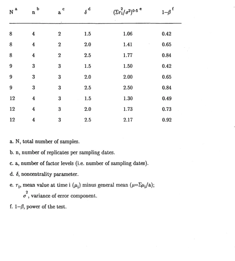
Montgomery (1984) gives the power curves for these tests. Table 2 presents

values of the power (1-,8) derived from sorne values of n, a, h' and

2 2

(~Ti/ (J )0.5. The table shows that the power increases (for any specified

value of h') as the number of replicates increases for the same numher of

sampling dates; if the number of sampling dates is not the same it is difficult

to compare the powers of the respective sampling strategies as the expression

2

([~Ti/ (J2]0.5) does not contain the same number of terms. The direct

comparison of power of trend analysis tests and ANOVA tests by comparing Tables 1 and 2 cannot he made. However, under the following circumstances a comparison of power between the statistical tests can he obtained.

Comparison of power, Trend analysis versus ANOVA.

To compare the power of trend analysis tests and ANOVA tests it is

2

necessary to relate the ampli tude of the trend ~ and the term ~Ti associated

with temporal changes of the mean. This is straightforward if time intervals

for successive samplings is the same and if there is a change of ~ between the

sampling intervals for both trend analysis and ANOV A. Even if the actual

2

time intervals are different, ~ and ~Ti can be related. In the case of Lac

Laflamme the time interval between successive samplings of the snowcover was approximately one week (6-10 days) in both 1985 (regression analysis)

Table 2. Power of the F -tests utilized in the analysis of variance. 8 8 8 9 9 9 12 12 12 b n 4 4 4 3 3 3 4 4 4 c a 2 2 2 3 3 3 3 3 3

a. N, total number of samples.

1.5 2.0 2.5 1.5 2.0 2.5 1.5 2.0 2.5

b. n, number of replicates per sampling dates.

1.06 1.41 1.77 1.50 2.00 2.50 1.30 1.73 2.17

c. a, number of factor levels (Le. number of sampling dates).

d. h, noncentrality parameter.

e. Ti' mean value at time i (JLi) minus general mean (JL=LJLi/a);

2 .

(J , varIance of error component.

f. 1-/3, power of the test.

f 1-/3 0.42 0.65 0.84 0.42 0.65 0.84 0.49 0.73 0.92 1-14

and 1988 (ANOVA).

Between two successive sampling dates, ANOVA is reduced to the

standard Student l-test which leads to the following relationship between ~

2

and ETi ,

=

±[+12

=

~2

₍₅₎

i=l

with j.t = (j.tl +j.t2 )/2 and ~ = j.t2 -j.tt since there is a change of ~ units

between two sampling dates. In a similar way it can be shown that for more

than two successive sampling dates (a>2) the general relationship between ~

2

and ETi is given by equation 6.

a _{.2 ~2}

a _{E . (a-i)}

L~=

1=1 1

a (6)

i = 1

By using tables 1 and 2, and equations 5 and 6 one can now compare the relative efficiency of the two statistical methods to detect changes in a dynamic system (e.g. the cold snowcover) for the same number of

observations. For example it can been seen from Table 1 that for a power

value of .40 (8 observations, b = 2.0 ) the regression analysis will detect a

slope of ~ = .310". For the same number of observations (N = 8) and

approximately the same value for the power of the ANOV A test of .42 2 2

(Table 2, n=4, a=2, {l = 1.5), the term (ETi/O" )0.5 is 1.06. Substituting

2 2 2 .

(1.06) 0" for ETi in equation 5 leads to a value of ~=1.50", the ANOV A test

in this case can thus only detect a slope of 1.50" from the same sample size.

The comparison is, however, only valid if the variance of the error

2

component (0") is the same for both methods.

In the above example the data for the ANOVA tests were obtained on two successive samplings of 4 replicates per sampling date (n = 4, a = 2,

Table 2). Equation 6 permits the comparison between the ANOVA test, for which the successive sampling dates are more than 2, and the trend analysis. Table 2 shows that the value of the power term for the condition of N = 9, n

= 3, a = 3 and li' = 1.5 is very similar (0.42) to the regression test (0.40) and

the ANOV A test (0.42, N=8, n=4, a=2, and 6' =1.5) cited above. If we

consider that the numher of observations are approximately the same (N = 9

2

V N = 8) then from the value of {bTi/o2)0.5 of 1.5 and equation 6 it can be

shown that the efficiency of the ANOVA can he bettered to detecting trends

of amplitude, il = 1.10',4 times out of 10 with the ANOVA (n=3, a=3) but

the trend analysis is still the most efficient method for the detection of a change in the concentrations.

Results and discussion. 1985: Trend detection

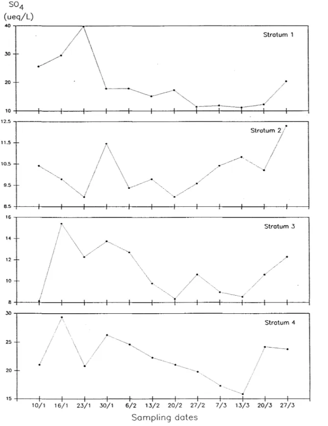
Table 3 shows the SWE, concentrations of S04 at each sampling date, and the mean concentration for the study period of four adjacent strata in the snowcover at the Lac Laflamme site between January 10 and March 27, 1985. The table also reproduces the weighted concentrations of S04 for the strata combined as one stratum. The study of the composite stratum smooths out the irregularities that occur hetween individual strata and represents a better picture of the overall evolution of that part of the snowcover where the strata are found. Although there may he a consistent monotonie trendover the whole time period the different strata may be exposed to different phenomena at different times. Thus one stratum may indicate a decrease in the concentration of S04 due to emigration of aerosols during snow metamorphism which is reflected by an increase in the S04 concentration of the adjacent stratum. In addition dry deposition will

increase the S04 particulary in those strata which comprise the surface of the pack early on in their existance even though the net dominant overall

phenomenom may result in S0410sses for the whole pack.

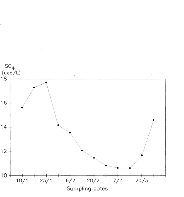
The graphical representation of the results of each individual stratum are presented in Figure 3; Figure 4 records the overall evolution of the strata combined as one stratum. Strata 1,3, and 4 (Figure 3)seem to show a

decrease between January 23 and March 13 while the behaviour of stratum 2

2-T~ble 3. S04 concentrations (p.eq 1-1_{) of four adjacent strata and of the composite stratum}

(strata 1-4) in the snowcover at Lac Laflamme, January to March, 1985.

])ate Stratum Stratum Stratum Stratum Stratum

10 Jan 16 Jan 23 Jan 30 Jan 6 Fév 13 Fév 20 Fév 27 Fév 7 Mar 13 Mar 20 Mar 27 Mar Mean 1 25.6 29.6 39.8 17.9 17.9 15.2 17.3 11.5 11.9 11.3 12.3 20.4 19.2 30.5 2 10.4 9.8 9.0 11.5 9.4 9.8 9.0 9.6 10.4 10.8 10.2 12.3 10.2 56.1 3 8.1 15.4 12.3 13.8 12.7 9.8 8.3 10.6 9.0 8.5 10.6 12.3 11.0 36.7 4 21.0 29.4 20.8 26.3 24.6 22.3 21.0 19.8 17.3 15.8 24.2 23.8 22.2 7.8

a. Snow water equivalent measured un millimeters

1-4 13.9 17.1 17.8 14.5 13.2 11.8 11.5 10.9 10.8 10.6 11.6 14.9 13.2

S04 (ueq/L) ~.---~---~ _{... /\} ... ...•.•. ...-30 \ , \. 20

\

.•.•..•. -... - ... ... Stratum 1 .-...• . _._. ____ ... _____ ._ ... __ , .. ...-P.----.. ·-.. ·· 10+----+----~--~--_+----+_--~--~----+_--_+----r---~--_+--~ 12.5 . . . - - - _ _ , Stratum 2/ 11.5 10.5 ···fi· 9.5 8.5+----+----~--~--_+---+_--~--~----+_--_+--~r_--~--_+--~

16...---Stratum 3 14 12 10 8+----+----r---1----+----+_--~--~----+_--_+--~r_--~--_+--~ ~...---, Stratum 4 25 20 15+_---+----r_--1----+----~--~--~----+_--_+--~r_--~--_+--~ 10/1 16/1 23/1 30/1 6/2 13/2 20/2 27/2 7/3 13/3 20/3 27/3 Sampling dates 1-18

Figure 3. Evolution.of S04 concentrations (J.req 1-1) in four adjacent st rata in the

snowcover, Lac Laflamme, Quebec, January to March, 1985 (sampling dates are schematic only).

S04

(ueq/L)

18~---. 16 14

•

.... ~ ...• 12 ...•.. ...• .. ...•...• 10+---+---~~---4---+--~--~'---+---+--~--~--~~

10/1

23/1

6/2

20/2

7/3

20/3

Sampling dates

Figure 4. Evolution of weighted S04 concentrations (peq 1-1

) in the composite stratum

(strata 1 to 4, Fig. 3), Lae Laflamme, Quebee, January to Mardl, 1985 (sampling dates are schematie only).

is more erratic. Figure 4 also indicates that the overall trend between

January 23 and March 13 is a decrease in 804 of approximately 7 ,.req 1-1; as

there was no loss or gain in 8WE for this specific cold period the loss

represents 39% of the original 80410ad in the pack.

Regression analyses, however, on all the data for the strata show that the trends are significant only in the case of the first stratum and the

composite stratum (Table 4). The overall trend of 804 losses is confirmed

for the composite stratum. 8pearman tests give exactly the same conclusions

thus showing that no aberrant data affected the regressions. If only the data

between January 23 and March 13 are subjected to the same analysis then

strata 3 and 4 also show a significant downward trend in 804 concentrations.

The results of the test lead us to the conclusion that there is a significant and progressive 10ss of 804 from the snow strata during the cold period. The increase in 804 concentrations at the beginning of the period may have been

due to dry deposition at the pack surface (Cadle et al. 1985); the pack

became deeper as the winter progressed, the lower strata (1-4) became

isolated from the atmosphere, and dry deposition ceased to have a direct influence on the chemical evolution of these strata. On the other hand, the general increase of 80 4 at the end of the period is due to the percolation of meltwater from the upper part of the pack during the start of the springmelt season.

1988: ANOV A analysis.

Table 5 shows the replicate values, the mean value, and the standard deviation of 804 concentrations for the four strata at the Lake Laflamme site in 1988. The weather in that year consisted of melt and rain-<>n-snow episodes and a prolonged period for the study of changes in cold snow did not occur. The longest period of persistent cold weather was experienced

between February 5 and February 15. These unfavorable weather conditions

did not allow the sampling of a stratum for more than two sampling dates. The 8tudent 1-test showed that there was a significant change over time of

80 4 concentrations for strata 2,3, and 4 during their respective cold periods.

In each case, los ses (18%, 2; 39%, 3; 27%,4) of S04 were registered; the

amplitude of the losses thus averages out at between 2.5% and 4% day-l.

2-T~ble 4. Regression tests and trend detection results of S04 concentrations in four

adjacent strata and the composite stratum(l-4) in the snowcover at Lac Laflamme for the period January 10 to March 27, 1985.

Stratum 1 2 3 4 Composite 1_4 Significant Trend (Yes/No) Yes, negative No No No Yes, negative

a.

A,

estimated slope, measured in p,eq t 1_week-1

-D.86 +0.06 -D.1I -D.21 -D.26 A b u 3.57 0.51 1.25 1.94 1.03

1-22

2-Table 5. S04 concentrations (p.eq 1-1)of four distinct strata in the snowcover of Lac Laflamme for different time periods, January 20 to March 4, 1988.

Stratum Stratum Stratum Stratum

1 2 3 4 20-1-88 20-1-88 5-2-88 23-2-88-Replicate #1 11.98 46.92 7.25 10.00 Replicate #2 11.40 50.65 7.29 10.42 Replicate #3 11.42 51.33 7.31 11.67 Replicate #4 11.52 50.98 7.33 10.83 Replicate #5 11.81 50.46 7.46 10.72 Mean 11.63 50.06 7.33 10.73 ~a _{0.26 1.80 0.08 0.62} 27-1-88 27-1-88 15-2-88 4-3-88 Replicate # 1 11.77 43.73 4.92 8.33 Replicate #2 11.90 41.13 4.52 7.92 Replicate #3 11.79 40.31 4.13 7.92 Replicate #4 11.42 40.38 4.33 7.92 Replicate #5 12.13 39.33 4.33 8.13 Mean 11.79 40.99 4.44 8.04 ~a 0.26 1.67 0.30 0.19

The tests also permitted the estimation of standard deviations of the error

component: the values are 0.26 treq 1-1_{, stratum 1; 1.74 treq 1-}1_{, stratum 2;}

0.22 treq 1-1, stratum 3; and 0046 J.req 1-1, stratum 4.

Comparison of the two methods, 1985, 1988.

From the above estimations of (J for i-tests and regression analysis we

can now compare the power of the tests to detect absolute changes in the

concentrations of 804 over time. Table 4 shows that the values of

q

for 804

concentrations varied between 0.51 J.req 1-1 and 3.57 treq 1-1 for the regression

analysis of snow strata sampled in 1985. In general the values of

q

are

proportional to the absolute values for the mean concentrations showing that the coefficient of variation is relatively stable. This is also true in the case of the ANOVA for the snow strata in 1988 (Table 5). We Can thus compare, on one hand, the power of the two methods for strata which have low

concentrations of 804, and, on the other hand, for strata which are more polluted in 804.

In the first case, stratum 2 in the 1985 series (S04 ~ 10 J.req 1-1, Table

3)) can be considered as being equivalent in mean to stratum 4 (S04 ~ 10 treq

1-1) in the 1988 ANOVA study. To estimate the powers of the different tests

used the estimated values of the standard deviations of error component are

q

= 0.51 treq 1-1_{, 1985, (Table 4) and}

q

_{= 0046 treq 1-}1_{, 1988.}

In the second case, stratum 4, 1985 (S04 ~ 20 treq t 1), the most

consistently concentrated stratum of the regression analysis, can be

compared with sorne limitations to stratum 2, 1988 (S04 ~ 40 J.req 1-1), the

most polluted stratum in 804 used for the ANOV A. Estimated values for

q

in this case are 1.9 J.req 1-1 in 1985 and 1.7 J.req 1-1 in 1988.

For the sake of comparison, the number of total samples taken (N) is set at 8. This represents 1 sample per date for 8 successive samplings in the regression analysis and 4 replicate samples per date for two samplings in ANOVA within the same time period. Substituting the respective values for

q

of strata 2 and 4, 1985, into Table 1 (regression analysis), and strata4 and

2, 1988, into Table 2 (ANOVA) permits the calculation of the amplitude of detectable changes over time of S04 concentrations at comparable powers.

Thus Table 6 shows that at a power of 0040 the regression analysis can detect

1-24

Table 6. Comparison of the power (1-,8) of regression analysis tests and of ANOVA tests

to detect trends of absolute amplitude (tre<l1-1) in S04 concentrations.

a) Low concentrations of S04 (~ 10 J-req 1-1)

N 8 8 8 1.5 2.0 2.5 0.12 0.16 0.20 Regression Analysis 1-,8 0.25 0040 0.55 ANOVA 0.69 0.92 1.15 1-,8 0042 0.65 0.84

b) High concentrations of S04 (> 20 J-req 1-1₎

N 8 8 8 1.5 2.0 2.5 0044 0.59 0.74 Regression Analysis 1-,8 0.25 0040 0.55 2.61 3047 4.36 ANOVA 1-,8 0042 0.65 0.84

relatively dilute snow. The ANOVA test, however, detects values of!:l. of onIy more than 0.69 J.teq 1-1 per sampling interval for similarly dilute snow at

the same power. For polluted snow strata the regression analysis at a power of 0.40 cau detect a trend amplitude of 0.59 p.eq 1-1 per sampling interval compared to 2.61 p.eq 1-1 per sampling interval by the ANOVA test at the same power.

Conclusion

The results of the 1985 and the 1988 studies clearly show that losses of

S04 cau occur in snow during cold periods. Analysis of the data also

demonstrates that for the same number of samples, the maximal distribution of the total number of samples over time (Le. 1 sample per sampling date), and regression analysis, is more efficient in detecting the chemical changes in snow than the alternative method of regrouping the number of samples for a lesser number of successive sampling dates and using ANOVA.

This information can be used to plan future sampling programs of cold snow. Two senarios for sampling can be envisaged. The first senario is that in which the cost of the field sampling is the major financial burden of the study .. If one has a prior knowledge of the variability of concentrations of

S04 in the snow, a minimum value for the amplitude of the changes that are detectable for the particular study in question may be set. By constructing tables similar to Table 6, the relationship between the number of samples, the maximum number of sampling trips that the budget will permit, the amplitude of the trend that is desired, and the probable success rate of detecting the trend (power of the test) for ANOVA may be found.

Conversely, if the number of samples is restricted by the budget but the field sampling is not, then a table of the power to detect the required amplitude of chemical change by regression analysis may be drawn up. This methodology, however, is only of value in simple systems e.g. in regions where the

probability of prolonged cold periods is high (Arctic, Antarctic). In the Lac Laflamme area the probability of accurately forecasting cold periods of more than one week or so is very 10w; in addition, the budget costs for analysis of samples and field sampling are comparable. In general, the program of snow sampling at this site relies more extensively on the ANOV A approach the lost of power is then offset by fewer field samplings and lower probability of

unfavorable weather conditions. On the other hand the study of chemical changes in cold snow in the laboratory where experimentaI conditions may be easily controlled (Jones, and Deblois 1987) is more amenable to regression analysis.

Acknowledgements

This research was made possible with the financiaI aid of Environment Canada and the N aturaI Sciences and Engineering Research Council of Canada.

References

Bickel,P.J., and K.A. Doksum. 1977. Mathematieal Statisties: Basie Ideas

and Seleeted Topies. Oakland: Holden-Day.

Box,G.E.P., and G.M. Jenkins. 1976. Time Series Analysis: Foreeasting and

Control. Revised Edition. Oakland: Holden-Day.

Cadle,S.H., J.M. Dash, and N.E. Grossnickle. 1984. Retention and release of chemical species by a northern Michigan snowpack. Water, Air and Soil Pollution 22:303-319.

Colbeck,S.C. 1981. A simulation of the enrichment of atmospheric pollutants in snow coyer runoff. Water Resourees Researeh 17(5):1383-1388. Conover,W.J. 1971. Praetieal Non-Parametrie Statisties. 2nd Edition. New

York: John Wiley.

Delmas,V., and H.G. Jones. 1987. Wind as a factor in the direct

measurement of the dry deposition of acid pollutants to snowcovers. In Seasonal Snoweovers: Physics, Chemistry, Hydrology. Eds. H.G. Jones and W.J. Orville-Thomas, NATO ASI Series C, Volume 211:321-335.

Hirsch,R.M., and J.R. Slack. 1984. A non-parametric trend test for seasonaI data with seriaI dependence. Water Resourees Researeh 20:727-732. Jeffries,D.S., and W.R. Snyder. 1981. Variations in the chemical composition

of the snowpack and associated meltwaters in central Ontario. In

Proceedings of3Sth Eastern Snow Conference. Syracuse, N.Y.:B.E.

Goodison.

Jones,H.G., M. Tranter, and T.D. Davies. 1989. The leaching of strong acid

anions from snow during rain-on-snow events: evidence for two

component mixing. Atmospheric Deposition (Proceedings of the

Baltimore Symposium, May 1989). IAHS Publ. NO.179:239-250. Jones,H.G. 1987.Chemical dynamics of snowcover and snowmelt in a Boreal

Forest. In Seasonal Snowcovers: Physics, Chemistry, Hydrology. Eds.

H.G. Jones and W.J. Orville-Thomas, NATO ASI Series C, Volume 211:531-574.

Jones,H.G., and C. Deblois. 1987. Chemical dynamics of N-rontaining ionic species in a boreal forest snowcover during the spring melt period.

Hydrological Processes 1:271-282.

Jones,H.G., and W. Sochanska. 1985. The chemical characteristics of snowcover in a northern boreal forest during the spring run-off

period. Annals of Glaciology 7:167-174.

Jones,H.G., and M. Bisson. 1984, Physical and chemical evolution of

snowpacks on the Canadian Shield (winter 1979-1980). Verh.

Internat. Verein. Limnol. 22: 1786-1792.

Lettenmaier,D.P. 1976. Detection of trends in water quality data from

records with dependents observations. Water Resources Research

12:1037-1046.

Montgomery,D.C. 1984. Design and Analysis of Experiments. Second Edition.

New York: John Wiley.

Netter,J., and W. Wasserman. 1974. Applied Linear Statistical Models.

Hemewood: Richard D. Irmin.

Ratkowsky,D.A. 1983. Nonlinear Regression Modeling. New York: Marcel

Dekker.

Tranter,M., et al. 1986. The composition of snowfall, snowpack and

meltwater in the scottish highlands : evidence for preferential elution.

CHAPITRE II CHAPTER II

SNOQUAL, a model for the simulation of meltwater quantity and quality in boreal fore st catchments: a study of the model

variants for the chemistry of snow meltwaters.

(SNOQUAL, un modèle pour simuler la quantité et la qualité des eaux de fonte dans des bassins de la forêt boréale; une étude de trois

versions du modèle pour la chimie des eaux de fonte)

H.G. Jones

INRS-Eau, Université du Québec, CP 7500, 2700 Einstein, Ste-Foy, Québec, Canada, G1V 4C7

J. Stein

Faculté de forestrie et de géodésie, 0870 Vachon, Université Laval, Québec, Canada, G1K 7P4

W. Sochanski

INRS-Eau, Universite du Québec, Carrefour John Molson, 2800 rue Einstein, Ste-Foy, Québec, Canada, G1X 4N8

II-2

Résumé

Le modèle conceptuel SNOQUAL, établit le rapport entre la quantité et la composition chimique des eaux déchargées du couvert de neige en période de fonte. Le modèle est structuré à partir de deux modules. Le premier, SNOW-17, est quantitatif; il simule le taux de décharge des eaux de fonte selon

l 'échange d'énergie à l 1 interface neige-atmosphère. Le deuxième est qualitatif; il utilise les extraits de SNOW-17 pour calculer la concentration des ions dans chaque volume de fonte par temps de pas utilisé. Ce deuxième module est dérivé des expressions de lessivage de divers espèces ioniques du couvert de neige par

les eaux de fonte. Le module qualitatif est caractérisé par un ou des coefficient(s) de lessivage (k) dont la valeur peut être différente selon l'espèce ionique lessivée.

Cet article décrit trois versions du module qualitatif qu10n a comparé pendant la calibration du SNOQUAL. Il s'agit de SNOQUAL1, SNOQUALR et SNOQUALD. Ces versions tiennent compte respectivement du processus de lessivage surficiel des crystaux de neige, du lessivage surficiel et de la charge ionique résiduelle qui se trouve à l 1 intérieur des grains, du lessivage surficiel de neige et du lessivage relativement plus lent du débris forestier sur le couvert de neige.

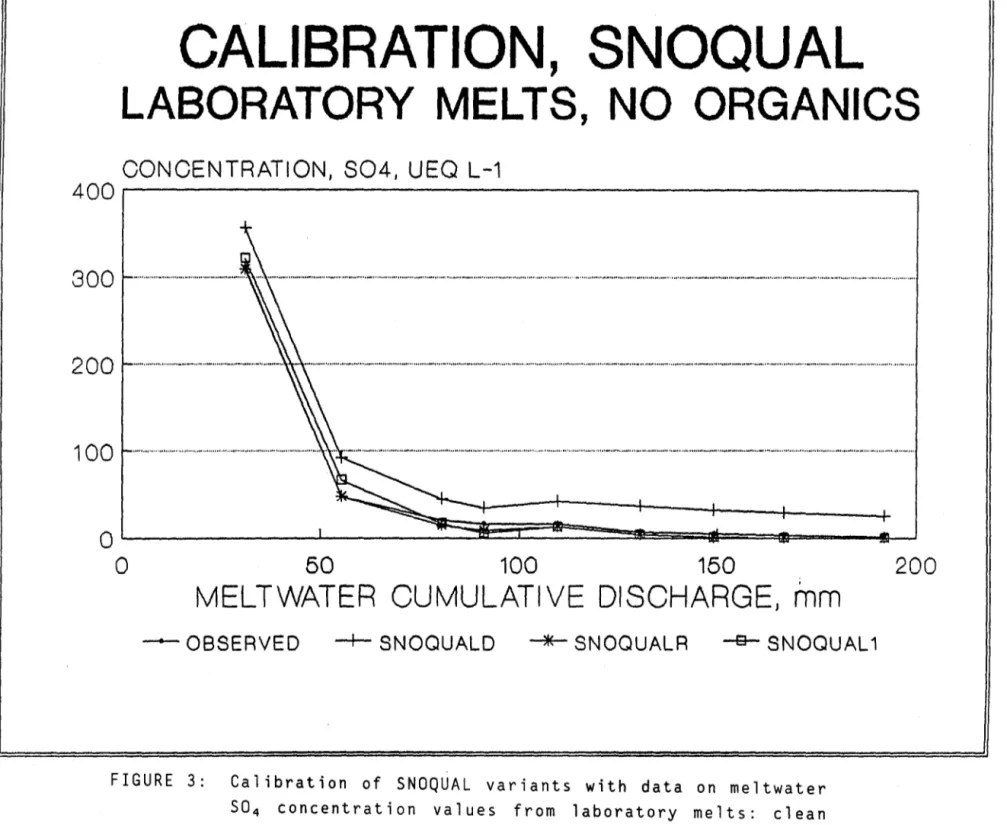
La calibration de chacun de ces modules qualitatifs par l'utilisation des données des fontes prises "in situ" au Lac Laflamme, Québec, et des fontes contrôllées en laboratoire démontre que les valeurs pour les coefficients de

lessivage sont influencées par la quantité de débris organique dans le couvert. De plus, les résultats démontrent que le module qui simule le mieux les

Enfin, on décrit les résultats d'une application du 5NOQUALR pour la simulation de l'acidité (pH) des premières eaux de fonte des couverts hivernaux accumulés

à partir de neige précipitée sous des conditions théoriques. Ces conditions

sont soit d'une réduction soit d'une augmentation des émissions de 502 par

11-4

ABSTRACT

SNOQUAL is a conceptual model that relates the quantity of meltwater released from the snowpack to the chemical composition of the discharge. The structure of the model consists of two modules. The first, SNOW-17 (Anderson, 1973), simulates the rate of meltwater discharge from the estimation of energy exchange across the snow-air interface. The second module takes the output from SNOW-17 and calculates the concentration of ions in each discrete

discharge by a routine which is derived from a, or two, first order leaching expression(s) for the soluble species from the snowpack. The qualitative module is characterized by a leaching coefficient(s) (k) the value of which can differ for each ionic species present in the pack leachate.

This paper discusses three versions of the qualitative module that have been used in the calibration of SNOQUAL. These three variants (SNOQUAL1, SNOQUALR, and SNOQUALD) attempt to reflect the physical reality of the interaction of meltwater and the snow in situ. They take into account, respectively, the leaching process of ice crystals, the suficial leaching plus the non-surficial ionic load which resides within the ice structure, and the presence of both rapid and slow leaching components (snow and canopy debris) in forested snowpacks.

The calibration of each of these qualitative modules with snow meltwater concentrations in laboratory and field experiments at Lac Laflamme, Quebec, shows that the leaching coefficients of the model variants are influenced by the quantity of organic debris in the pack. The results also show that the model which best generates meltwater concentrations close to those measured in the field is SNOQUALR.

The application of SNOQUALR to the simulation of the acidity (pH) of the first meltwaters that can be expected from snowpacks deposited under condition of either a reduction or an increase in S02 emissions is also given.

INTRODUCTION

In the southeastern region of the Canadian Shield the pH of the precipitation is often in the range of 3.8-4.5. These levels of acidity are judged to be detrimental to the aquatic and terrestrial ecosystems of the area. In the

"Réserve faunique des Laurentides" north of Quebec City, Environment Canada has established an experimental program on the measurement and impact of acid

precipitation on the aquatic ressources of the Lake Laflamme watershed (Jones and Deblois, 1987). One of the major research projects of the program is the modelling of the fluxes of acid waters through the watershed during the spring melt. The mean pH of the waters of Lake Laflamme is 6.4 during the greater part of the year; it is only during the spring melt period that the lake waters undergo episodic acidification. pH values of 4.2 for sub-ice waters in inshore spawning areas have been recorded (Charette et al., 1984).

The model development has centered mainly on the construction of a

comprehensive model for the acidity of lake waters. The model is modular and consists of a snow meltwater model (SNOQUAL) which serves as the input to a

model of soil solution chemistry (SOILEQ). The output from SOILEQ is th en used

to model the movement of meltwaters through the lake (the model SHOREMIX). A

hydrological model VSAS2 based on the variable source area concept is used to simulate the meltwater pathways in the watershed from the time penetrates to

11-6

first is SNOW-17 which simulates quantitatively meltwater discharge from the snowpack. The second module simulates the release of chemical components from the snow by the meltwaters.

This paper describes the meltwater leaching of snow and other in-pack material, the basic process variable of the chemical model. The various versions of the model which have been used to simulate the chemical composition of meltwaters discharged from the snowpack at Lake Laflamme are discussed. The difficulties in the calibration of the models using field data are outlined and the accuracy of the different versions of the model to generate the concentrations of the

strong-acid anions SO~- and NO; in meltwaters are compared. Laboratory studies

to determine the probable range of values for the leaching parameter of ionic species from the melting snowpack are also described.

STUDY SITE AND METHODOLOGY

The site: Lac Laflamme is a small headwater lake (0.06 km-2 ; location, 47°19'

N, 71°07'W) in the Parc des laurentides, Quebec (Fig. 1). The watershed ( 0.6

km-2 ) is covered with close-knit mature stands of Balsam Fir interspersed with

small areas of birch and spruce. The trees are heavily covered with epiphytic lichens. The mean annual temperature is 0.2°C (-15°C January; 15°C, July).

The total snowfall (October-May) at Lac Laflamme is approximately 400 mm (Snow

Water Equivalent, SWE) and the pack usually attains a depth of 120-150 cm at the end of the accumulation period. During the winter the pack receives considerable amounts of canopy fallout consisting mostly of lichens, bark, needles, leaves and small twigs (Jones and Deblois, 1987). The melt season

47 LAKE LAFLAMME'.

•

LAKE TANTARE

•

CASSETTE RIVER

•

/

/

-/

--1

~'....F~~~--t-MONTRÉAL ~-~

(-__ .r--J

- 0

---_

.. ---.1

1 ;

U.$. A 401~-•• - •• 50Iun

,

f ' , --.. ï.,... .. .../

FIGURE 1: Study Site, Lac Laflamme, Québec.

9°

•

\

t

11-8

generally begins towards the end of April and maximum meltwater discharge occurs during the first two weeks of May.

Field snowcover and meltwater study: four square shaped lysimeters (1 m by 1 m; sidewall height, 0.5 m) were installed for the 1988 melt season. The

lysimeters were constructed of plastic covered fiberglass (Fig 2). Three were placed within a 8alsam Fir stand under a closed canopy, an open canopy (50% coyer), a mixed canopy of 8alsam Fir and White 8irch. The fourth lysimeter was placed in clear-cut area. The extent of the canopy coyer was determined by photography (subtended angle of view, 23°) of the canopy coyer from the forest floor. Snowcover samples were taken in the vicinity of the lysimeters using an Adirondack corer. Precipitation was sampled by means of a Sangamo wet-only collector. Meltwater samples representing the integrated sample of all

meltwater discharges over 24 hours were ta ken at midday (noon to 14:00 hours) every day. All samples were kept at DoC during transport to the laboratory; pH and conductivity measurements were taken on arrival and the samples filtered and conserved for further chemical analysis (Jones, 1987).

Laboratory study: a simulator for snowmelt discharge was constructed of plastic; the simulator consisted of four columns within which IIcleanll _snow

taken from open areas in the forest, and different combinat ions of clean snow and organic debris could be melted under carefully controlled conditions (Jones and Deblois, 1987). Between 80-100 cm of snow or snow-organic mixtures were placed in the columns and the melt conditions were adjusted to give meltwater discharges similar to those observed in the field. The amount of organic matter added to the clean snow (weight per unit area of snow surface) was approximately equal to that found on the snowcover at the Lac Laflamme site

FIBREGLASS LYSIMETER ( 1

m x

1

m

x

50

cm )

DISCHARGE TUBE (ABS 7.5

cm ,00. )

t-'---:z:..-STEEL ORUM (200 L )

t-'--t---z::.._ PLASTI C REel PIENT

(45 L )

CEMENT BLOCK

FIGURE 2: Field lysimeter, Lac Laflamme, Québec.

...

... 1

II-la

just prior to the springmelt. As in the case of the field lysimeters the

meltwater samples were gathered every 24 hours and analysed in exactly the same manner.

Chemical analysis: the samples were analysed for the major ions (Na, K, Ca, Mg, Cl, S04' N0_{3 );} details of the precise methods used may be found in Jones and Sochanska, 1985. The washing of field lysimeters with distilled water showed that contamination of meltwater by the collectors was not a feature of the experimental set-up; the laboratory lysimeters, however, did show sorne

contamination (Cl) probably due to sorne microbiological degradation of the PVC used to construct the columns.

MODEl PROCESSES

The models are chemical subroutines of the global model for the simulation of snow meltwater quantity and quality (SNOQUAL, Stein et al, 1986). They are based both on the physical phenomena that are known to occur when snow meltwaters move down through the pack and on observations of meltwater composition from meltwater studies in the field (Jones, 1987) and the

laboratory (Jones and Deblois, 1987). The models are of three types all of which, however, are based on the physical concept of the leaching of solubles from the pack matrix by a diminishing reserve of ice meltwaters. In all of the models the parameter for the rate of leaching is a leaching coefficient 'k ' (Foster,1978).

In the first model (SNOQUAL1) the value of the leaching coefficient represents the net leaching effect of the removal of solubles from both the surface of

snow crystals and other material (mostly fallout of organic matter from the

canopy) in the pack. In the case of field studies the contribution of solubles

from organic matter to the total amount of matter leached from the pack may be

appreciable e.g. K+. Conversely, organic matter may also show an apparent

effect of adsorption of sorne ions e.g. N0₃ due to microbiological assimilation

of nutrients in situ during the melt period (Hoham et al, 1989).

In the second model (SNOQUALR) the value of the leaching coefficient again represents the net leaching effect of solubles from the pack; the snow and organic matter being lumped together. However, in this particular model the material to be removed from the snowpack is segregated into two components. The first component consists of concentrated solutions of ionic species on the surfaces of snow grains. The segregation and concentration of ionic solutions on the surfaces of the grains is known to occur during the metamorphism of snow crystals to grains prior to the melt season (Tranter et al, 1986). This

process, however, leaves sorne of the ions as a residual component of the original composition of the snow crystals within the ice lattice structure of the snow grains. This residual component may be easily shown from laboratory leaching experiments.

For the purposes of the modelling of snow meltwater chemistry, the residual component is not classed as a leacheable material as such, but rather is the basic contribution of the melting ice to the overall chemical composition of meltwaters. As the melting snow removes more and more of the concentrated surface solutions from the snow grains (plus surface leaching of organic

matter), the composition of the meltwaters discharged from the pack approaches that of the residual concentrations in the ice lattices of the snow grains.

11-12

This residual component is expressed by means of a constant, R, the

fractionation coefficient. Although it is convenient to adopt this concept of segregation of solubles in the pack based on the results of the laboratory experiments on "clean" snow, field studies on meltwaters cannot distinguish between residual solubles within ice grains and those which may be removed by the meltwaters from organic matter in the later stages of the melt.

The third model (SNOQUALD) is similar to (SNOQUALR) in that the model

segregates the material to be leached from the pack into components. In this

model, however, a distinction is not only made between surface leachables and residual concentrations in the ice structure but also between snow and other pack components (e.g. organic matter, dry deposited material). A constant, s, the segregation coefficient, is used to distinguish between the contribution of the snow to the meltwater composition and that of the other matter. The model thus contains two leaching coefficients, ks and km' representing respectively the leaching of snow and the leaching of the other components, particularly the organic matter. Laboratory studies are carried out in an attempt to distinguish the two coefficients; curve fitting will also optimise the values

MODEl STRUCTURES

In all the models the common model parameters are the concentration of ions in

the snow, C (~eq 1-1_{) , the height of the pack, H (snow water equivalent, SWE,}

mm), and k (net leaching coefficient, mm-1_{) or k and k in the case of}

s m

SNOQUALD. Model inputs are Co' the bulk ionic concentration of the snow prior

height of the pack at the end of a specified melt period. The leaching

coefficient(s), K, can either be an input or an output, the latter being the result of curve-fitting of the numbers generated by the models to the real data of snow and/or meltwater compositions in the field. Ci the concentration of an ionic species in the snow at the condition H

=

Hi is the primary output which transposed into the meltwater concentration, Cm' is used as the basis for the curve fitting exercises to determine other model parameters (Jones et al,

1986).

The expressions 1, 2, and 3 represent SNOQUAL1, SNOQUALR, and SNOQUALD respectively.

-k (H -H.)

C.

=

C e 0 1 (1)

-k (H -H.)

Ci

=

C o(l-R)s e S O l 1 0

-k (H -H.)

e 0 1 _{+ RC} o (2)

-k (H -H.)

C o(l-R)(l-s)e m O l + RCo (3)

ln SNOQUALR the term, R, the fractionation coefficient is either an input to the model, the value being determined from laboratory studies, or an output, the value being determined by default during the calibration procedure. In SNOQUALD, R, is an input determined from observations in the field or the laboratory (the value of R is usually calculated as the mean value of measured concentration in the last 10-20% of the residual meltwaters. In this model, the second constant, segregation coefficient, s, which quantifies that part of the