arXiv:1409.1690v2 [astro-ph.SR] 8 Mar 2016
X-ray emission from magnetic massive stars
1Ya¨el Naz´e
∗GAPHE, D´epartement AGO, Universit´e de Li`ege, All´ee du 6 Ao ˆut 17, Bat. B5C, B4000-Li`ege, Belgium
V´eronique Petit
Dept. of Physics & Space Sciences, Florida Institute of Technology, Melbourne, FL, 32901, USA
Melanie Rinbrand
Department of Physics & Astronomy, University of Delaware, Bartol Research Institute, Newark, DE 19716, USA
David Cohen
Department of Physics & Astronomy, Swarthmore College, Swarthmore, PA 19081, USA
Stan Owocki
Department of Physics & Astronomy, University of Delaware, Bartol Research Institute, Newark, DE 19716, USA
Asif ud-Doula
Penn State Worthington Scranton, Dunmore, PA 18512, USA and
Gregg A. Wade
Department of Physics, Royal Military College of Canada, PO Box 17000, Station Forces, Kingston, ON K7K 4B4, Canada
ABSTRACT
Magnetically confined winds of early-type stars are expected to be sources of bright and hard X-rays. To clarify the systematics of the observed X-ray properties, we have analyzed a large series of Chandra and XMM-Newton observations, corresponding to all available exposures of known massive magnetic stars (over 100 exposures covering ∼60% of stars compiled in the catalog of Petit et al. 2013). We show that the X-ray luminosity is strongly correlated with the stellar wind mass-loss-rate, with a power-law form that is slightly steeper than linear for the majority of the less luminous, lower- ˙M B stars and flattens for the more luminous, higher- ˙M O stars. As the winds are radiatively driven, these scalings can be equivalently written as relations with the bolometric luminosity. The observed X-ray luminosities, and their trend with mass-loss rates, are well reproduced by new MHD models, although a few overluminous stars (mostly rapidly rotating objects) exist. No relation is found between other X-ray properties (plasma temperature, absorption) and stellar or magnetic parameters, contrary to expectations (e.g. higher temperature for stronger mass-loss rate). This suggests that the main driver for the plasma properties is different from the main determinant of the X-ray luminosity. Finally, variations of the X-ray hardnesses and luminosities, in phase with the stellar rotation period, are detected for some objects and they suggest some temperature stratification to exist in massive stars’ magnetospheres.
1. Introduction
As they lack deep outer convective envelopes, dy-namos analogous to the Sun’s are not expected to op-erate in early-type stars (A, B, O). Magnetic fields were however found in a few percent of the popula-tion of main sequence A and late B-type stars in the Galaxy (Wolff 1968; Power et al. 2007) and, more re-cently, in a similar proportion of early B and O stars (Hubrig et al. 2011; Wade et al. 2013, and references therein). While they are most probably fossil fields, their detailed origin remains elusive (primordial field, early dynamo, binary mergers, Ferrario et al. 2009; Braithwaite 2013; Langer 2013). The detected mag-netic fields share similar properties: they are generally strong (a few kG), organized on large scales (i.e., with important dipole component), and globally stable on timescales of at least years.
Such strong, organized magnetic fields are able to channel the stellar wind flows towards the magnetic equator, giving rise to regions of magnetically confined wind (MCW) and creating a stellar magnetosphere (Shore & Brown 1990; Babel & Montmerle 1997a; ud-Doula & Owocki 2002). The presence of these dense confined winds leads to additional emissions or absorptions throughout the electromagnetic spectrum. In the high-energy range, X-rays should arise from the collision between the high-velocity wind flows chan-neled from both hemispheres along the magnetic field lines (e.g. Babel & Montmerle 1997a).
Indeed the observed properties of θ1Ori C (O7Vfp, Ku et al. 1982; Schulz et al. 2000; Gagn´e et al. 2005) agree well with theoretical expectations (Babel & Montmerle 1997b; Gagn´e et al. 2005). The X-ray emission is overluminous by one dex compared to similar non-magnetic stars and is dominated by a thermal compo-nent at ∼3 keV, compared to 0.2–0.6 keV in ‘normal’ O stars. Furthermore, the X-ray lines are narrow and on average unshifted while the line ratios indicate a for-mation region close to the photosphere, as expected for slow-moving material trapped in a magnetosphere. Si-multaneous X-ray and optical variations further under-line the link between MCWs and X-rays (Gagn´e et al. 1997, 2005). While some details of the observations are not yet reproduced by models2, the overall
agree-*Research Associate FRS-FNRS
1Based on data collected with XMM-Newton, and Chandra. 2The emitting plasma is located too close to the photosphere;
unex-plained variations of the X-ray absorption are observed as the view-ing angle of the magnetosphere changes; the observed X-ray line
ment is still quite satisfactory. θ1Ori C thus appears as a prototype for understanding magnetospheres of slowly-rotating massive stars.
For cooler and more rapidly rotating objects,
σOri E (B2Vp) appears as another well-studied land-mark. Its emission is also hard and luminous in the X-ray range (Sanz-Forcada et al. 2004; Skinner et al. 2008), although no details on its X-ray lines are yet available. The properties of σ Ori E are roughly repro-duced by models (Townsend et al. 2007) and even the predicted magnetic braking has been detected obser-vationally for this object (Townsend et al. 2010).
These two prototypes are not the sole magnetic objects observed in the X-ray range. However, the other objects conform less well to the theoretical ex-pectations. The magnetic Of?p stars display order-of-magnitude ray overluminosity, some narrow X-ray lines, and correlated X-X-ray/optical changes but their high-energy emission is dominated by soft X-rays rather than hard ones (Naz´e et al. 2004, 2007, 2008, 2010, 2012a). τ Sco (B0.2V) displays an over-luminosity, a relatively hot (1.7 keV) component, nar-row and unshifted X-ray lines formed close to the star (Mewe et al. 2003; Cohen et al. 2003). However, the relatively complex magnetic topology of the star (Donati et al. 2006) was expected to generate strong variability of the X-ray emission with the rotational pe-riod, which was not observed (Ignace et al. 2010). Fi-nally, Oskinova et al. (2011) compared the X-ray prop-erties of a sample of 11 magnetic B stars, including
σOri E (see above), β Cep (Favata et al. 2009), LP Ori and NU Ori (Stelzer et al. 2005), while Ignace et al. (2013) analyzed new X-ray observations of two τ Sco analogs. The situation again appears quite varied: some objects displayed hard X-ray emission, while others rather emit soft X-rays; overluminosity seemed to be the exception rather than the rule. No obvious correlation was found by Oskinova et al. (2011) be-tween the high-energy properties and bolometric lu-minosity, magnetic field strength, rotation period, or pulsation period (when existing). Therefore, the origin of the discrepancy between observations and models remains unknown.
The situation thus appears less satisfactory than the few iconic magnetic objects would at first suggest. In order to clarify the situation, the detailed correla-tion between magnetic/stellar properties and the X-ray widths are slightly too large; small shifts of X-ray lines are observed throughout the rotation cycle, but are not predicted Gagn´e et al. 2005
characteristics should be assessed systematically for a larger sample of stars, notably searching for poten-tial differences in X-ray observables related to their magnetospheric structure. To do so, we examine the overall sample of magnetic massive stars whose stel-lar and magnetic parameters are generally well known (Petit et al. 2013). Section 2 presents the X-ray ob-servations used in this study and the analysis method, Sections 3 and 4 describe the observational results and their interpretation while Section 5 summarizes our findings and concludes this paper.
2. Observations
Several X-ray observatories have flown since the 1970s. However, their instruments had various capa-bilities, not always comparable. In this study, we aim to maximize the number of detections while ensur-ing the highest possible homogeneity in the analysis (i.e. similar spectral resolution and energy band). We searched Swift and Suzaku archives for observations of the magnetic stars of Petit et al. (2013) but, with the exception of τ Sco (Ignace et al. 2010), no source was detected by these facilities. We also found ASCA de-tections for five of our targets, but these objects lie in clusters, where the coarse PSF of ASCA makes it dif-ficult to extract uncontaminated data. We thus focused our work on CCD spectra in the 0.5–10.0 keV band, which allows us to detect hard emissions. Our analysis is based on XMM-Newton-EPIC and Chandra-ACIS data, with a mix of targeted programs (notably our own programmes, PI Naz´e and PI Petit) and serendipitous archival observations. There are more than a hundred exposures available for 40 targets. Therefore X-ray ob-servations are available for 63% of the Petit et al. cat-alog. Table 1 provides the stellar/magnetic properties of the sample, from Petit et al. (2013), whereas Table 2 provide the detailed information on the X-ray obser-vations.
It is of interest to examine the location of our sam-ple in the magnetic confinement-rotation diagram de-scribing the dynamical structure of magnetospheres (Fig. 1, see also Petit et al. 2013 for further details). Although we do not have observations of the entire catalog of Petit et al. (2013), our targets are well dis-tributed: we are thus not sampling a particular sub-population amongst the known magnetic massive stars, and our conclusions on the magnetic OB stars should therefore have a general character.
XMM-Newton data were reduced with SAS v13.0.0
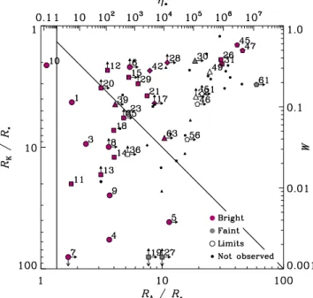
Fig. 1.— Location of the targets in the magnetic confinement-rotation diagram (see Fig. 3 of Petit et al. 2013, for the identification of all individual stars). The confinement parameter η∗ = B2pR2∗/(4 ˙Mv∞) and
the Alfven radius RA(R∗) ∼ 0.3 + (η∗+ 0.25)1/4 are
given as top/bottom abscissa, respectively. The right and left ordinates show the ratio of rotation speed to orbital speed W and the Kepler corotation radius RK = W−2/3R∗, respectively (see e.g. Petit et al. 2013,
for more discussion about these parameters). Highly confined winds of rapidly rotating stars therefore ap-pear at the top right of the diagram. The symbol shapes represent spectral types (circles: O-type stars, squares: B-type stars with Te f f >22 kK, triangles:
B-type stars with 19< Te f f < 22 kK, pentagons:B-type
stars with Te f f <19 kK, diamonds: Herbig Be stars).
Darker symbols correspond to objects with brighter X-ray emission (see Sect. 2: “bright” objects are those studied spectroscopically).
using calibration files available in June 2013 and fol-lowing the recommendations of the XMM-Newton team3. Data were filtered for keeping only best-quality data (PAT T ERN of 0–12 for MOS and 0–4 for pn) and discarding background flares affecting the obser-vations. A source detection was performed on each EPIC dataset using the task edetect chain on the 0.4– 10.0 keV energy band and for a likelihood of 10. This task searches for sources by using a sliding box and determines the final source parameters from point-spread-function (PSF) fitting: the final count rates cor-respond to equivalent on-axis, full PSF count rates. When sources displayed high count rates, the possi-bility of pile-up was assessed using the pattern dis-tribution (task epatplot): datasets with non-negligible pile-up were discarded and do not appear in Table 2. For the remaining observations, we then extracted EPIC spectra using the task especget for circular re-gions centered on the best-fit positions of the sources and regions as close as possible to the targets for the backgrounds. The background positions as well as the extraction radii were adapted taking into account the crowding near the source as well as the off-axis PSF degradation. EPIC spectra were grouped, using specgroup, to obtain an oversampling factor of five and to ensure that a minimum signal-to-noise ratio of three (i.e. a minimum of 10 counts) was reached in each spectral bin of the background-corrected spec-tra. Note that for σ Ori E, only the events outside the flare were considered, as this flare is probably due to a low-mass companion (Sanz-Forcada et al. 2004; Bouy et al. 2009).
The Chandra ACIS observations were reprocessed following the standard reduction procedure with ciao version 4.54. The procedure is similar to the one de-scribed for EPIC observations. Source where searched with the celldetect tool and the count rates where deter-mined with aprates. The ACIS spectra and responses where extracted using the standard specextract with re-gions centred on the source with background rere-gions as close as possible to the target. The spectra were grouped in the same fashion as the EPIC spectra. The presence of pile-up was estimated from the count rate per frame, and exposures with non-negligible pile-up were discarded.
Of the 40 magnetic massive stars with X-ray
obser-3SAS threads, see
http://xmm.esac.esa.int/sas/current/documentation/threads/
4CIAO threads see http://cxc.harvard.edu/ciao/threads/.
vations, six B stars (ALS3694, HD 55522, HD 36485, HD 306795, HD 37058, HD 156424) remain unde-tected while five other ones (Tr16-13, HD 163472, ALS15956, HD 37017, HD 175362) have only very faint detections and the last object, ALS8988, a ques-tionable detection5. For XMM-Newton, the equivalent on-axis count rates associated with faint detections as well as the 90% detection limits throughout the field-of-view were automatically calculated during the source detection process. For the Chandra observa-tions, the number of counts, count rates, and their associated 1σ errors at the position of these targets were estimated from aperture photometry by the task aprates, with a Bayesian estimation of the background. The one-sided, 90% upper limits are taken as 1.28σ in case of non-detection. Corrections for incomplete PSF and effective area from the Chandra manual were then applied to obtain the final estimate of the upper lim-its6. The Chandra and XMM-Newton count rates were then converted into fluxes (corrected for ISM absorp-tion) using WEBPIMMs. To this aim, we used models combining the individual interstellar absorption (with-out additional absorption) and one thermal component. For the latter, several temperatures between 0.3 and 2.0 keV, as found suitable for most other B stars (see below), were tried and they yielded comparable re-sults. Table 3 provides the derived X-ray luminosities and LX/LBOLratios.
A total of 28 magnetic stars have at least one X-ray spectrum usable for spectral modelling (i.e. 44% of the Petit et al. catalog). These spectra were fitted within Xspec v12.7.0 with the aim of using homogeneous fit-ting procedures to get homogeneous and comparable results. We fitted the spectra using absorbed optically-thin thermal plasma models, i.e. wabs × phabs ×
Papec, with solar abundances (Anders & Grevesse
1989). The first absorption component represents the interstellar column, which was fixed to 5.8 × 10²¹ × E(B − V) cm−2 (Bohlin et al. 1978, see Table 1). The second absorption allows for possible additional (lo-cal) absorption, e.g. due to the stellar wind (con-fined or not). Regarding the emission components, two
5The X-ray detection of ALS8988 was first reported by
Townsley et al. (2003) but a longer Chandra exposure resolved the emission into two sources, each separated by 2” from the B star position, casting doubt on the detection of X-rays from ALS8988 (Wang et al. 2008). We thus discard this source from our sample and do not discuss it further.
6A factor of two correction was also applied to HD 36485, which
was observed with ACIS-S+HETG (resulting from the redirection of 50% of the flux into towards the gratings)
methods were used. The first uses one or two optically-thin thermal models with free temperatures. Two ther-mal components were only used if a single component did not provide a satisfactory fit. In this case, input temperatures of 0.45 and 1.0 keV were used as first guesses. The second method considers a given set of four absorbed optically-thin thermal plasma models, this time with fixed temperatures of 0.2, 0.6, 1.0, and 4.0 keV. This set of temperatures was chosen to mini-mize erratic results and to ensure a good representation of the X-ray emissions of the magnetic stars. Tables 4, 5, and 6 provide the parameters of the best fits. We also provide the observed fluxes in 3 energy bands and their associated fluxes corrected for the interstellar ab-sorption, with 1σ error bars7. It must be noted that the results described in the next sections are consistent when using either fitting method.
For the brightest objects in the sample, the reduced
χ2 of the best-fit are sometimes larger than 2, hence are formally not acceptable. We however kept these results notably because, even in these cases, the fitting was good in the 0.5–10.0 keV energy band where the flux was estimated. Most of the problems in such cases probably results from nonsolar abundances and/or un-realistically small error bars (that do not account for the calibration systematics). In some cases, we fixed one or several spectral parameters. This typically hap-pened when: (1) the additional absorption was very low (< 1019cm−2) and its associated error was unreal-istically large (∼ 1023cm−2) - the absorption was then fixed to zero, and (2) several spectra of the same target were available (see Sect. 4.3) - we identified the best-fit parameters (absorption and/or temperature(s) and/or normalizations, depending on the source’s behaviour) which were not significantly varying throughout expo-sures and we used them as fixed parameters for a sec-ond fit of the individual exposures. This allows us to clarify the observed trends by avoiding erratic results (especially when individual spectra display a low num-ber of recorded counts) and removing the uncertainty in temperature coming from its interplay with absorp-tion.
7These errors were calculated using Xspec error command for
spec-tral parameters or flux err command for observed fluxes. When the error bars were asymmetric, the largest value is given here. As is usual in Xspec, these errors do not adequately take into account the interactions between spectral parameters and errors on dered-dened fluxes cannot be formally calculated (as some information is missing, e.g. the error coming from the good/bad choice of model). Note that unrealistically large errors may sometimes be derived, es-pecially when the additional absorption is close to zero.
Once X-ray spectra have been fitted, the next step is to evaluate how the X-ray emission of magnetic stars relates to the MCW phenomenon, through the compar-ison of specific parameters. Three main observables are available for each spectral fitting: the level of X-ray emission, its spectral shape, and its absorption. We examine each one in turn in the following sections, and then determine the variability properties of the targets, when possible.
3. The X-ray luminosity of magnetic massive stars 3.1. Observational results
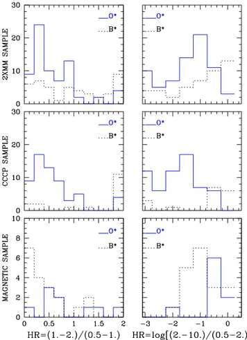
In our sample, we observed a large range of X-ray luminosities and log[LX/LBOL] ratios. Fig. 2 compares the observed values for our sample of magnetic mas-sive stars with two large samples of OB stars: Chandra Carina Complex Project (CCCP, Naz´e et al. 2011) and the 2XMM survey (Naz´e 2009)8. There are some ob-vious differences.
First, the X-ray observations of a particular region (e.g. Carina, but see also NGC6231, Sana et al. 2006) have rather high detection limits, leading to a high cut-off in the luminosities: while this generally has lit-tle impact on O star detectability, many B stars with faint X-ray emission are thus missed. In our sample, some deeper exposures are available, notably because of observations acquired by the authors, and this leads to the detection of much fainter X-ray emission (Fig. 2). Second, for “normal” single, non-magnetic O stars, embedded wind shocks lead to LX/LBOLof about 10−7 (Fig. 2, Berghoefer et al. 1997; Naz´e 2009; Naz´e et al. 2011, and references therein) while larger values are observed for the magnetic stars.
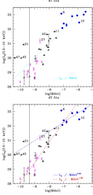
To better understand the phenomena at work, we searched for correlations between the X-ray luminosi-ties and the stellar/magnetic parameters, first and fore-most the mass-loss rates. Indeed, since every wind shock mechanism extracts kinetic energy from the wind flow and converts it to thermal energy (partly radiated away as X-rays) at shock fronts, we expect some scaling of the X-ray properties with wind mass-loss rate ˙M. Fig. 3 (top panel) shows that there is of course a strong trend of LXvs. ˙M (from Table 1), al-beit with a fair amount of scatter. In particular, a linear
8Note that these samples are not fully representative of non-magnetic
single stars, as they are contaminated by a few X-ray bright colliding wind binaries and a few magnetic objects (which are also included in our sample).
Fig. 2.— X-ray luminosities (corrected for ISM absorption) and LX/LBOL ratios of massive stars in 2XMM (Naz´e 2009, top panel) and CCCP (Naz´e et al. 2011, middle panels) compared to values for stars in this paper (4T fits, bottom panels). The solid blue lines refer to O stars, and the black dotted ones to B stars. Note that the shift in average log[LX/LBOL] between CCCP and 2XMM comes from the different analysis choices (see Naz´e et al. 2011, for a discussion of this problem).
Fig. 3.— X-ray luminosity (corrected for ISM ab-sorption, from 4T fits) as a function of mass-loss rate. Filled blue dots correspond to O stars, black empty triangles to B stars, magenta crosses and downward-pointing arrows to faint detections and upper limits on the X-ray luminosity, respectively. The labelled line on the top panel illustrates a LX∝ ˙M relation, whereas we show on the bottom panel the best-fit relations (see text and Table 7). Stars of particular interest are la-beled according to their identification number in Table 1.
Fig. 4.— Ratio between the X-ray luminosity and the bolometric luminosity as a function of mass-loss rate or bolometric luminosity. Symbols are as in previous figure.
relation between log(LX) and log( ˙M) does not seem to hold for the low/high extreme values of the mass-loss rates. Looking at the log[LX/LBOL] values (Fig. 4), we can more clearly distinguish two groups of ob-jects with different behaviours, one with a high value of log[LX/LBOL]∼ −6.2 notwithstanding the mass-loss rate (group 1) and one with log[LX/LBOL] varying with log( ˙M) or log(LBOL) (group 2).
The first group comprises all of the O stars and six B stars with log[LX/LBOL]> −6.6 (see IDs in Fig. 3). These objects seem to follow the LX ∝ M˙0.6 relation for radiative shocks in high-density winds (Owocki et al. 2013) even if three of them (#31, #45, and #47) have very low mass-loss rates. We may also note that two particular cases amongst the O stars, #6 Plaskett’s star (higher luminosity) and #10 ζ Ori (lower luminosity)9. The particular properties of these two O stars could be due to the possible non-magnetic ori-gin of their X-rays. For Plaskett’s star, not only there is a close companion to the magnetic star but there may be an X-ray bright collision of their stellar winds (Linder et al. 2006). For ζ Ori, the strength of the mag-netic field is low, hence its impact on the stellar wind is weak and its X-rays may thus come from embedded wind-shocks, as in non-magnetic stars: the very “nor-mal” X-ray properties of this star (no overluminosity, softness of the emission) confirm this view.
Group 2 consists of the remaining 13 B stars, which follow a significantly steeper trend in mass-loss rate than those in the first group.
We determined the best-fit power-laws between log(LX) and log( ˙M) using least squares for these two groups (Fig. 3 and Table 7). It should be noted that, despite not being included in their derivation, the points corresponding to upper limits and faint de-tections match well these relations (Figs. 3 and 4).
The mass-loss rates used for this study were de-rived from the Vink et al. (2000) recipe and thus actu-ally correspond to theoretical magnetosphere feeding rates. To use a more “observational” value, we have also derived the relations with the bolometric luminos-ity log(LBOL) (Fig. 4 and Table 7). Since the wind is driven by radiation, both types of relations (with ˙M and LBOL) yield similar results, but it should be noted that the correlations are slightly tighter for log( ˙M) than for log(LBOL), which is why we will focus on the for-mer ones in the following.
9It must be noted that considering or excluding these two stars from
We examined whether alternative relations (e.g. with wind density, traced by ˙M/4πR2
∗v∞) would yield
tighter correlations, but that was not the case. We also examined the relation between the X-ray lumi-nosity and the maximum strength of the Hα emis-sion, which should reflect the quantity of material in the magnetosphere, but the latter did not appear to be a good discriminant either10. Finally, we exam-ined relations including additional parameters, such as magnetic field strength or magnetospheric size, e.g. log(LX) = a × log( ˙M) + b × log(Bp) + c, but they
did not result in significantly better fits. This may be due to more complex relations with secondary pa-rameters (see next section) as well as the different ranges covered by the parameters in our sample: ter-minal velocities v∞ cover a 760–3600 km s−1 interval
(i.e. variations by 0.7 dex), magnetic field strengths Bp cover a larger 0.2–20 kG interval corresponding
to 2 dex variations (excluding the extremely low field of ζ Ori), while bolometric luminosities log(LBOL/L⊙)
cover a range 2.8–5.8 (i.e. 3 dex variations) and mass-loss rates ˙M are between 10−10.4 and 10−5.5M
⊙yr−1
(or 5 dex variations). It is thus quite normal for the bolometric luminosity or the mass-loss rate to be the main discriminant for the predicted X-ray luminosi-ties, although the field strength and terminal velocity could explain some of the scatter around the relations shown in Figs. 3 and 4.
3.2. Comparison with theoretical predictions The MCW shock model was first discussed in de-tail by Babel & Montmerle (1997a) on the basis of the confined magnetosphere scenario of Shore & Brown (1990). While most directly aimed at understanding a single star (IQ Aur), the paper of Babel & Montmerle (1997a) also presented a formula to predict the X-ray luminosity of magnetic massive stars with power-law dependences on the three basic parameters mag-netic field strength, wind velocity, and mass-loss rate: LX = 2.6 1030B0.4∗ M v˙ ∞ where the magnetic field B∗
is expressed in units of kG, the mass-loss rate ˙M in units of 10−10M
⊙yr−1and the terminal velocity v∞in
units of 1000 km s−1. Fig. 5 compares the predictions from this formula (listed in Table 1) with the observed X-ray luminosities in the 0.5–10.0 keV energy band af-ter correcting for inaf-terstellar absorption. The observed
10O stars have similar log[L
X/LBOL] but a large range of Hα strengths,
whereas B stars have Hα equivalent widths close to zero but a large range of log[LX/LBOL] values
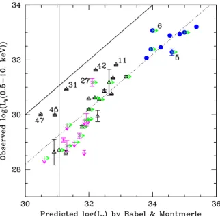
and predicted luminosities appear to be globally cor-related (confirming the hints of Oskinova et al. 2011), but two remarks should be made.
The first and main one is that the Babel & Mont-merle formula fails to reproduce the observed trends. Indeed, a steeper-than-unity slope relates the observed and predicted luminosities for low X-ray luminosities (Fig. 5). This is related to our finding of two relations, LX∝ ˙M0.6or LX∝ ˙M1.4, rather than one. Second, the predicted values are on average 1.8 dex higher than the observed ones, for both groups (as illustrated in Fig. 5). This may be partly due to the definition of instru-mental bandpass (Babel & Montmerle were analyzing ROSAT data but never explicitly stated the bandpass to which their formula applies) but also to some idealiza-tion of the physics involved (notably a nearly perfect shock heating efficiency).
The pioneering work of Babel & Montmerle has long been the sole one available, but recently a new study by ud-Doula et al. (2014) re-investigated the subject, this time considering specific instrumental bandpass and including more precise physics through the use of 2D MHD simulations. They notably found that properly accounting for the post-shock cooling length steepens the relationship at low mass-loss rates through a shock retreat effect11. Additionally, at high ˙M, the reduced confinement for a given dipolar strength makes the LX vs. M relation become shal-˙ lower, and may even turn over at the highest values of the mass-loss rate. These trends are indeed seen in our data.
As MHD simulations are computationally costly, and nearly impossible for η∗∼104−106confinement
values appropriate for many observed magnetic B stars, ud-Doula et al. (2014) developed a semi-analytic “XADM” model, which predicts the X-ray luminosi-ties as a function of magnetic field strength, stellar radius, and wind velocity. It reproduces well the over-all trends in the MHD-computed LX vs. M but the˙ idealized XADM analysis, which assumes 100% ef-ficiency, display larger values than the MHD results. This reflects a reduced X-ray efficiency (.20%) from infall and other dynamical effects in the full 2D MHD
11When channelled winds from opposite footpoints collide near the
loop apex, the cooling layer where X-ray emission arises extend from loop top to the shock. In low density plasma, this shock is “re-treated” back into the accelerating wind, because of the inefficiency of radiative cooling (cooling length comparable to Alfven radius). This effect is thus more pronounced for B stars with low-density winds.
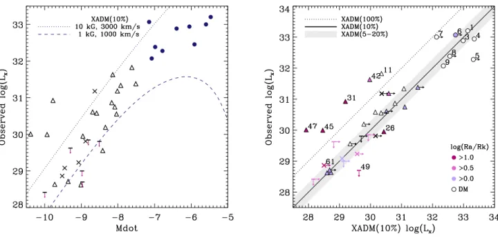
Fig. 6.— Left: Relation between the X-ray luminosity in the 0.5–10.0 keV band (corrected for ISM absorption, from 4T fits) and logarithm of mass-loss rate. The dotted and dashed lines represents predicted X-ray luminosities in the same energy band using the XADM model (ud-Doula et al. 2014), scaled by 10%, for a single value of the stellar radius of 1012cm and two set of (indicated) magnetic field and wind parameters bracketing the parameters of our sample. Symbols are as in Fig. 3. Right: Comparison between the observed X-ray luminosity of magnetic stars (as in left panel) and the predicted values using the XADM model of ud-Doula et al. (2014). The dotted line illustrates the ideal model with 100% efficiency whereas the solid line indicates a scaling by 10%; the grey shaded area corresponds to scalings by 5–20% (a range in efficiency consistent with MHD models). Rightward-pointing arrows indicate stars for which the dipolar field strength is a lower limit. The symbols are colour-coded according to the predicted size of their centrifugally supported regions caused by rapid rotation (with darker shades for larger sizes); stars without predicted centrifugal support (see Petit et al. 2013) have empty symbols. Stars of particular interest are labeled according to their identification number in Table 1. Note that ζ Ori (#10) is not present on this plot as the XADM model is only valid for stars with significant magnetic confinement (i.e., η∗>1).
Fig. 5.— Comparison of the X-ray luminosities of magnetic stars (corrected for ISM-absorption, from 4T fits) with the predicted values using the formula of Babel & Montmerle (1997a). Green rightward-pointing arrows indicate lower limits on the predicted luminosities when only lower limits on the dipolar field strengths are known, the solid line corresponds to a 1-to-1 correlation while the dotted line is located 1.8 dex below, other symbols are as in Fig. 3.
simulations, implying that a scaling of the XADM model is necessary. The left panel of Fig. 6 shows that predictions by this model, scaled by 10% and for parameters bracketing the most extreme combinations of magnetic field and wind velocity in our sample, bracket well the observed data. To explore the effects of additional model parameters, we computed the X-ray luminosities using the individual parameters of our targets (see last column of Table 1 and the right panel of Fig. 6): a good agreement is found, with less scatter than in Figs. 3 and 5.
The overall observed emission levels suggest effi-ciencies in the range of 5–20% (grey area in Fig. 6), with a best-fit around 10%. Note that refining this value will notably require more precise determinations of the mass-loss rates since both a lower ˙M and a lower efficiency similarly lead to a lower X-ray emission. In-deed, detailed studies (e.g. Oskinova et al. 2011) often show significantly lower mass-loss rates than theory predicts and mass-loss rates of OB stars, generally in-ferred from density-squared diagnostics, could be low-ered by a factor of ∼ 3 to take into account the effects of wind clumping (Oskinova et al. 2008): the theoret-ical mass-loss rates used here may thus have to be re-vised downward.
A few discrepancies nevertheless exist between data and the predictions from ud-Doula et al. (2014), as can be noted in Fig. 6 by the presence of stars with over- or under-luminosities. Amongst O stars, the most discrepant point is NGC1624-2 (#5) which displays an X-ray luminosity lower by about 1 dex compared to the model prediction (see also Fig. 5). In this context, it must be recalled that the model does not take into account the absorption of the X-ray emis-sion by the cool wind material. However, the spectra of the O stars require such additional absorption to be reproduced by apec thermal models (see Sect. 4.2), which is not surprising in view of their dense stel-lar winds. Therefore, the amount of X-rays actually generated, which should be compared with the model, may be higher than the emergent X-ray emission level derived here. This effect, which may explain why the efficiency appears slightly lower for O stars than for B stars (Fig. 6), particularly applies to NGC1624-2 (#5) as this star hosts the largest magnetic field amongst O stars, hence the largest magnetosphere, and requires the highest absorption (1.2 × 1022cm−2, see Tables 4 and 5). Its generated X-ray emission level could easily be 1 dex higher (see Petit et al., submitted). The other apparently deviant point amongst O stars is HD 108
Fig. 7.— Left: Comparisons of the hardness ratios obtained with the two fitting choices: they are independent of the method, showing their robustness. Right: Relation between hardness ratios and temperatures (4T fits). There is no unique linear relationship between the two parameters, but an interesting dichotomy showing that two values of the same average temperature yield the same hardness ratio. Filled blue dots correspond to O stars, black empty triangles to B stars.
(#7), which appears brighter than expected (Fig. 6). However, the detailed magnetic properties of this ob-ject are not known, and the presence of an overlumi-nosity can thus only be truly ascertained after further monitoring.
There are also five B-type stars with observed lumi-nosities larger by at least one dex compared to the pre-dictions (Fig. 6): those are #11 τ Sco, #31 σ Ori E, #42 HD 200775, #45 HD 182180, and #47 HD 142184. This is unlikely to be due to the contamination by low-mass companions undergoing X-ray bright flares: the observed X-ray emission is mostly soft, and no flares are detected in their lightcurve. Another pos-sible origin for this discrepancy is the uncertainty in mass-loss rate, as the X-ray luminosity is a strong function of ˙M. Beyond remarks already made above, this particularly applies to stars near the bi-stability jump (22.5< Te f f <30 kK), but only one object out
of 5 belong to this category. A last possibility for ex-plaining the high luminosity of these stars is the role of rapid stellar rotation, which can contribute significant centrifugal acceleration to the pre-shock wind plasma (ud-Doula et al. 2008; Townsend & Owocki 2005) but is not included in the models of ud-Doula et al. (2014).
However, while four of these five B stars are among the rapid rotators with the most extreme magnetospheres (darker symbols in the right panel of Fig. 6), it is not a general rule, as the luminosity of some other rapidly-rotating objects are well reproduced by the model (e.g. #26, #49, or #61) and one overluminous star (i.e. #11) is not rapidly rotating. In the same vein, a mismatch also exists for τ Sco (#11) whose high-energy behaviour differs from those of its “clones” (#13 HD 63425 and #14 HD 66665, Ignace et al. 2013, and this work). Further investigation of the effect of rotation, combined with multi-wavelength detailed study of the individual stars to mitigate the mass-loss rate uncertainties would thus be useful. 4. Other X-ray properties
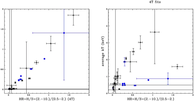
4.1. Hardness or temperature
Our fittings also characterize the spectral shape of the X-ray emission, through two parameters. The first one is a “hardness ratio” calculated as the ratio be-tween the hard (2.–10.0 keV) and soft (0.5–2.0 keV) ISM absorption-corrected fluxes. This hardness ra-tio appears very reliable as it is notably independent
Fig. 8.— Hardness ratios of massive stars in 2XMM (Naz´e 2009, top panels) and CCCP (Naz´e et al. 2011, middle panels) compared to values for stars in this pa-per (bottom panels). Note that one limit of the energy bands is different (2 keV in our data, 2.5 keV in CCCP and 2XMM).
of details of the fitting itself (see left panel of Fig. 7). However, when the source is both faint and rel-atively soft, the hard X-ray flux (hence the hardness ratio) may be underestimated. It is a problem which is difficult to solve without better observations, but it should be noted that it does not prevent us from de-tecting sources mostly composed of very hot plasma. The second parameter is the average temperature, de-fined as kT = (PkTi ×normi)/(Pnormi), where
normiare the normalization factors of the spectral fits,
i.e. 10−14R nenHdV/4πd2, listed in Tables 4 and 5.
This parameter is sometimes used as diagnostic for the properties of the X-ray emission of massive stars (Gagn´e et al. 2011; Ignace et al. 2013). However, we found it to be not as reliable as the hardness ratio (Fig. 7). Indeed, even for bright sources, there is a trade-off between absorption and temperature, which means that a unique spectral shape can be fitted by sev-eral solutions with very different average temperatures. This effect was reported several times in the past (e.g. Naz´e et al. 2007), even when high-resolution spectra were used (Naz´e et al. 2012a). In this work, we were regularly confronted with this problem, e.g. fits with similar hardness ratios but average temperatures of 0.2 and 1.0 keV fit equally well the spectra of σ Ori E. The main problem is that it is difficult to securely constrain independently the level of additional absorption: av-erage temperatures should thus not be taken at face value. Fortunately, the same conclusions are reached for both parameters, so that we present only hardness ratios in the following.
Our targets cover a wide (2 dex) range of hardness ratios (see e.g. Table 6). Compared to large samples of generally non-magnetic stars (Fig. 8), the magnetic O stars appear to have larger hardness ratios. Indeed,
ζOri has the lowest hardness ratio of our sample, con-sistent with the probably non-magnetic origin of its X-rays. The situation is different for B stars: the mag-netic B stars of our sample appear softer than most B stars in CCCP or 2XMM. However, as noted above, the CCCP and 2XMM sample mostly X-ray bright B stars, which may introduce an observational bias.
To assess the possibility of a link between the spec-tral shape and the emission level, Fig. 9 shows hard-ness ratios as a function of X-ray luminosities. The situation appears quite varied. O stars display various hardness ratios despite similar X-ray luminosities (and even more similar LX/LBOLratios). Most of the B stars display low (< 0.2) hardness ratios despite an extended range of luminosities though there are also a few
ob-jects displaying elevated hardness ratios compared to other stars of similar luminosities. Amongst them, we find three B stars with brighter than predicted X-ray emission (#31, #45, and #47) as well as two B stars for which observation and prediction agree (#17 and #35).
We searched for correlations between hardness/temperature and the stellar or magnetic parameters but none are found. From the theoretical point of view, the MCW shock mechanism should, in principle, result in higher plasma temperatures, because of the higher velocity jump in the head-on MCW shocks compared to those in stochastic embedded wind shocks. It is true that the emission of magnetic O stars appears, on average, slightly harder than that of “normal” O stars, but the scatter in each group is large. In addition, the situation is opposite for magnetic B stars, whose X-ray emis-sion is predominantly soft, even slightly softer than “normal” B stars. Detailed models by ud-Doula et al. (2014) further predict a harder X-ray emission for a higher confinement and/or a higher mass-loss rate but this theoretical prediction is not verified. Also, there is no obvious link between the detected overluminosities and hardness ratios (Fig. 10). These facts, together with the large scatter amongst O stars, suggest that the main driver for plasma temperature properties must be different than the main driver for the X-ray luminosity, which may guide future theoretical modelling. 4.2. Absorption
Another interesting observable to investigate is the additional, local absorption (i.e. above interstellar ab-sorption). For “normal” O stars, the high-energy emis-sion arises throughout the wind, whose cool parts may absorb X-rays. Some absorption effects are indeed de-tected, in the shapes of the line profiles (Cohen et al. 2010; Herv´e et al. 2013) as well as in the additional absorption needed to model spectra (with values up to 8 × 1021cm−2 and an average of 4 × 1021cm−2, see e.g. Naz´e 2009; Naz´e et al. 2011). No such additional absorption is needed to model the spectra of “normal” B stars (Naz´e 2009). However, as magnetic stars pos-sess dense magnetospheres, significant local absorp-tion might still be possible.
Except for the highest value (found in NGC1624-2, the most magnetic O star), the absorption values found for magnetic O stars are not significantly dif-ferent from what is observed in “normal” O stars. It may be noted that the O stars with the three highest absorptions also display the three highest hardness
ra-tios, pointing to absorption as responsible for elevated ratios, rather than temperature (Fig. 9 and Tables 4, 5). However, no correlation between absorption and the stellar/magnetic parameters could be found.
In a similar way, magnetic B stars do not generally require additional absorption, like their non-magnetic siblings. Whenever best-fits require additional absorp-tions (Tables 4 and 5), a fit with (forced) zero addi-tional absorption has a similar quality. There are how-ever two exceptions (#29 and #42). It is difficult to find a common point between these two objects, apart from the fact that they have both been reported to be Herbig stars - but they are not the only ones in our sample. Rapid rotation, associated with large and dense mag-netospheres, is not an explanation either, as the latter object is rapidly-rotating, but not the former, and other rapidly-rotating magnetic stars do not show such in-creased absorption.
4.3. Variability of the X-ray emission
To assess the presence of changes in the observed X-ray emission, several exposures are needed but in our dataset, only eight targets have more than one spectrum available. We have therefore examined this subsample, by searching for variability between the individual exposures (see Table 8 for a summary). It should be mentioned that this subsample represent only a small fraction of the Petit et al. catalog: the de-rived conclusions thus do not have a general character. 4.3.1. Stable X-ray emission: HD 148937, σ Ori E,
and ζ Ori
The observations (XMM-Newton only) of ζ Ori yield remarkably stable results. For HD 148937, there is also no significant difference between the two XMM-Newton observations, but the average tempera-ture appears 10% higher in the Chandra exposure, and the associated flux are about 15% lower. This is rem-iniscent of the results of Schellenberger et al. (2013) for isolated galaxy clusters. The detected changes therefore seem to be related to cross-calibration dif-ferences and cannot be attributed to the star without further information. A similar situation is found for
σOri E.
The constancy of the X-ray emission of these three objects can be attributed to their magnetic and geo-metric properties. HD 148937 has a low obliquity an-gle between the magnetic pole and the rotational axis, so that the variations of the line profiles in the
opti-Fig. 11.— Evolution of the average temperatures and hardness ratios (HR = H/S = FIS Mcor(2. − 10.0 keV)/FIS Mcor(0.5 − 2. keV)) as a function of observed fluxes for the three objects with many (> 6) observa-tions: HD 47777 (left), NU Ori (middle) and Tr16-22 (right). Red open symbols correspond to Chandra data, while black filled symbols correspond to results from XMM-Newton observations. The values shown here correspond to the results from 2T fits (results are similar for the 4T fits, and for ISM-absorption corrected fluxes). HD 47777 displays flux variations but no large spectral changes, whereas NU Ori and Tr16-22 display simultaneous flux and hardness variations.
cal domain are of very small amplitude (Naz´e et al. 2010; Wade et al. 2012a). This geometry also reduces the possibilities of change in occultation or absorption (see Sect. 4.3.3), explaining the stable X-ray emis-sion. For σ Ori E, the rotation period is short (1.19d, or 103ks) so that changes related to confined winds would be easily detected during a long exposure like the Chandra observation (91ks) but that is not the case (Skinner et al. 2008, see in particular their Fig. 5). This absence of phase-locked X-ray variations in
σOri E explains the stability of the X-ray emission when comparing XMM-Newton and Chandra datasets. It could be related to the large size of the magneto-sphere (about 31R∗for the Alfven radius), which
min-imizes the impact of occultations in the high-energy domain. Finally, the wind confinement of ζ Ori is very small, so that the wind is nearly undisturbed by the presence of the (small) magnetic field. Its X-ray emis-sion, most probably linked to embedded wind shocks as for non-magnetic O stars, is not expected to vary (cf. ζ Pup, Naz´e et al. 2013).
4.3.2. Flux variations without obvious spectral changes:
βCep and HD 47777
The observations of β Cep display small flux vari-ations, though the spectral shape (hence the average temperature and hardness ratio) appears stable. This confirms the analysis of Favata et al. (2009) of the same data. The available datasets were taken over 10d, an interval comparable to the rotation period (12d), but, without additional data, it is difficult to judge whether these small flux variations are truly correlated with the stellar rotation period: their origin remains uncertain.
HD 47777 also displays a quite stable spectral shape, but its flux varies by at least a factor of two (Fig. 11). A rotation period of 2.64d (about 228ks) was recently derived for this object (Fossati et al. 2014). The longest available exposures cover about half of that period (Table 2), and we therefore examined the X-ray lightcurves to search for variations compatible with it. None was detected, but ∼10ks flares at least tripling the X-ray emission level are observed in Chan-dra exposure #2540 and in XMM-Newton exposure #0011420101. Outside flaring episodes, the flux ap-pears less variable. It must be recalled that HD 47777 is a Herbig star, hence the presence of flares is not totally surprising (e.g. through the possible contami-nation by X-rays from a low-mass companion). Their link with the MCWs is certainly not established.
4.3.3. Flux variations with spectral changes: HD 191612, NU Ori, Tr16-22
The changes in HD 191612 were reported by Naz´e et al. (2007, 2010), and we confirm here the results of varying flux and spectral shape. These variations are clearly phase-locked, with the maxi-mum (resp. minimaxi-mum) flux occurring when the dense equatorial regions are seen face-on (resp. edge-on) (Naz´e et al. 2010).
Similar variations are seen for NU Ori (Fig. 11). In addition, the Chandra data systematically yield fittings with lower hardness ratios and lower average temper-atures, which is contrary to known calibration effects (Schellenberger et al. 2013). This suggests that the tar-get truly was softer when observed with Chandra.
Tr16-22 was observed more than 20 times in the X-ray range and shows clear flux and spectral shape variations (Fig. 11, and Naz´e et al. 2014). Changes are best seen on XMM-Newton data, because of their higher quality, their higher number, and the fact that they cover a large range of flux and hardness values. The large number of exposures helped us identify-ing, for the first time, the possible period of Tr16-22 (Naz´e et al. 2014).
Variations in both flux and spectral shape are thus detected for three stars, as well as for θ1Ori C (Gagn´e et al. 2005; Stelzer et al. 2005). Moreover, for HD 191612, θ1Ori C, and possibly Tr16-2212, the flux variations are clearly phased with the stellar rotation period, as demonstrated by the simultaneous minima in X-ray and optical emissions. This can be qualita-tively explained in the case of magnetic oblique ro-tators: as the view on the magnetosphere changes as the star rotates, occultation of the X-ray emitting re-gions by the star or obscuration by its confined wind can cause periodic variations, recurring with the stel-lar rotation period. However, the latter explanation can be discarded: a large increase in absorption would be required to explain the observed flux decreases, but no significant one (i.e. larger than 2–3σ) was detected during our spectral fitting nor for θ1Ori C, (Gagn´e et al. 2005, see in particular their Fig. 14). Moreover, if absorption was the cause of the flux vari-ations, the X-ray emission would actually always be softer when the flux is minimum, which is not the case (see below).
12The period of NU Ori is unknown, so that we cannot check the
We are thus left with the hypothesis of occultation as the main cause of the X-ray variations. In this case, the observation of simultaneous flux and hard-ness changes indicates that the X-ray production re-gion is somewhat stratified in temperature. However, HD 191612, Tr16-22, and NU Ori, appear harder when brighter, while θ1Ori C appears to be softer while brighter in the COUP data (see Fig. 7 in Stelzer et al. 2005), i.e. the opposite behaviour despite the fact that
θ1Ori C is not conceptually different from the three others. Since there are two hardness/flux trends, the in-ferred magnetospheric geometry must differ from star to star: for θ1Ori C, the warm plasma, responsible for the soft X-rays, is the one suffering most from occul-tation and should thus be confined in a smaller region; for the other stars, the hard X-rays should be produced closer to the photosphere and magnetic equator, ex-plaining their disappearance during occultations, while the soft X-rays should be produced in a larger region, less prone to such effects.
Up to now, the problem of flux or hardness changes was not addressed in published MCW models yet. The behaviours reported above therefore represents strong observational constraints, that can help guiding future modelling.
5. Conclusion
The goal of this analysis is to study the X-ray emis-sion of magnetic OB stars. With this aim, we have analyzed a large series of X-ray observations (more than 100 exposures), which cover ∼60% of the known magnetic massive stars listed recently by Petit et al. (2013). Spectra were extracted and fitted by thermal models whenever the sources were bright enough (28 cases). In addition, we converted the count rates into X-ray luminosities for 5 faint sources, while upper lim-its on the X-ray luminosities were derived for 6 unde-tected objects. Two O stars (ζ Ori and Plaskett’s star) show distinct X-ray properties, indicating that the main origin of their X-ray emission is most probably non-magnetic.
We analyzed the whole sample in quest of relations between X-ray properties and stellar/magnetic param-eters. The X-ray luminosities follow LX∝ ˙M0.6(hence log[LX/LBOL] is constant at −6.2) for O stars and a few B stars, and LX∝ ˙M1.4 for most B stars. Considering alternative relations or a two-parameter dependence of the luminosity, e.g. on mass-loss rate and magnetic field rather than on mass-loss rate only, does not
im-prove significantly the results. It must be noted that the observed X-ray luminosities, and their trends with mass-loss rates, cannot be explained within the frame-work of embedded wind shocks. On the other hand, luminosity predictions using the Babel & Montmerle (1997a) model of MCWs are too high (by 1.8 dex) and fail to reproduce the observed trends at high and low mass-loss rates. New MHD modelling of MCWs in-cluding shock retreat (ud-Doula et al. 2014) are how-ever able to match observations (level of X-ray emis-sion, trend with mass-loss rates) fairly well. There are nevertheless five B stars much more luminous than ex-pected: most of them are rapid rotators, but not all; in a similar way, not all rapid rotators are overlumi-nous. The origin of their intense X-ray emission thus remains uncertain, requiring more observational and theoretical work.
Regarding other observables, the situation appears less clear. Additional absorption is needed for fit-ting X-ray spectra from O stars and a few B stars, but no obvious correlation with stellar/magnetic prop-erties is detected. Spectral shape varies amongst the targets, but again, no obvious correlation with stel-lar/magnetic properties is detected, contrary to expec-tations of harder emission with higher confinement or mass-loss rate. Further theoretical work is thus re-quired to identify the missing ingredient explaining this (lack of) trends.
Finally, when several observations were available, we have examined the variability of the objects and observe three different behaviours. First, X-ray char-acteristics were found to be constant in some cases, as expected from the properties of the target (pole-on geometry for HD 148937, large magnetosphere for σ Ori E, non-magnetic origin of the X-rays for
ζOri). Second, flux changes without changes in spectral shape are observed in two cases (HD 47777 and β Cep) but they cannot be linked to the confined wind phenomenon using current data. Lastly, periodic changes in flux and spectral shape are also observed (e.g. HD 191612 and θ1Ori C). They are most prob-ably linked to occultation effects in magnetic oblique rotator systems and suggest various temperature strat-ification for the MCW regions.
Acknowledgments
YN acknowledges careful reading by G. Rauw, as well as support from the Fonds National de la Recherche Scientifique (Belgium), the Communaut´e
Franc¸aise de Belgique, the PRODEX XMM and In-tegral contracts, and the ‘Action de Recherche Con-cert´ee’ (CFWB-Acad´emie Wallonie Europe). VP ac-knowledges support from NASA through Chandra Award numbers G02-13014X and TM-15001C issued by the Chandra X-ray Observatory Center which is op-erated by the Smithsonian Astrophysical Observatory for and behalf of NASA under contract NAS8-03060. MR acknowledges support from NASA ATP Grant NNX11AC40G and from University of Delaware. AuD thanks NASA for support through Chandra Award number TM4-15001A. GAW acknowledge Discovery Grant support from the Natural Science and Engineering Research Council of Canada (NSERC). ADS and CDS were used for preparing this document.
Facilities: XMM, CXO. REFERENCES
Anders, E., & Grevesse, N. 1989, Geo. Chim. Acta, 53, 197
Babel, J., & Montmerle, T. 1997a, A&A, 323, 121 Babel, J., & Montmerle, T. 1997b, ApJ, 485, L29 Berghoefer, T. W., Schmitt, J. H. M. M., Danner, R., &
Cassinelli, J. P. 1997, A&A, 322, 167
Bohlin, R. C., Savage, B. D., & Drake, J. F. 1978, ApJ, 224, 132
Bouy, H., Hu´elamo, N., Mart´ın, E. L. et al. 2009, A&A, 493, 931
Braithwaite, J. 2013, Proc. of IAUS 302, arXiv:1312.4755
Cohen, D. H., Cassinelli, J. P., & Macfarlane, J. J. 1997, ApJ, 487, 867
Cohen, D. H., de Messi`eres, G. E., MacFarlane, J. J., et al. 2003, ApJ, 586, 495
Cohen, D. H., Leutenegger, M. A., Wollman, E. E., et al. 2010, MNRAS, 405, 2391
Donati, J.-F., Howarth, I. D., Jardine, M. M., et al. 2006, MNRAS, 370, 629
Favata, F., Neiner, C., Testa, P., Hussain, G., & Sanz-Forcada, J. 2009, A&A, 495, 217
Ferrario, L., Pringle, J. E., Tout, C. A., & Wickramas-inghe, D. T. 2009, MNRAS, 400, L71
Fossati, L., Zwintz, K., Castro, N., et al. 2014, A&A, in press, arXiv:1401.5494
Gagn´e, M., Caillault, J.-P., Stauffer, J. R., & Linsky, J. L. 1997, ApJ, 478, L87
Gagn´e, M., Oksala, M. E., Cohen, D. H., et al. 2005, ApJ, 628, 986 (see erratum in ApJ, 634, 712) Gagn´e, M., Fehon, G., Savoy, M. R., et al. 2011, ApJS,
194, 5
Herv´e, A., Rauw, G., & Naz´e, Y. 2013, A&A, 551, A83
Hubrig, S., et al. 2011, A&A, 528, A151
Ignace, R., Oskinova, L. M., Jardine, M., et al. 2010, ApJ, 721, 1412
Ignace, R., Oskinova, L. M., & Massa, D. 2013, MN-RAS, 429, 516
Ku, W. H.-M., Righini-Cohen, G., & Simon, M. 1982, Science, 215, 61
Langer, N. 2013, Proc. of IAUS 302, arXiv:1312.2373 Linder, N., Rauw, G., Pollock, A. M. T., & Stevens,
I. R. 2006, MNRAS, 370, 1623
Mewe, R., Raassen, A. J. J., Cassinelli, J. P., et al. 2003, A&A, 398, 203
Naz´e, Y., Rauw, G., Vreux, J.-M., & De Becker, M. 2004, A&A, 417, 667
Naz´e, Y., Rauw, G., Pollock, A. M. T., Walborn, N. R., & Howarth, I. D. 2007, MNRAS, 375, 145 Naz´e, Y., Walborn, N. R., Rauw, G., et al. 2008, AJ,
135, 1946
Naz´e, Y. 2009, A&A, 506, 1055
Naz´e, Y., ud-Doula, A., Spano, M., et al. 2010, A&A, 520, A59
Naz´e, Y., Broos, P. S., Oskinova, L., et al. 2011, ApJS, 194, 7
Naz´e, Y., Zhekov, S. A., & Walborn, N. R. 2012a, ApJ, 746, 142
Naz´e, Y., Bagnulo, S., Petit, V., et al. 2012b, MNRAS, 423, 3413
Naz´e, Y., Flores, C. A., & Rauw, G. 2012c, A&A, 538, A22
Naz´e, Y., Oskinova, L. M., & Gosset, E. 2013, ApJ, 763, 143
Naz´e, Y., Wade, G.A., & Petit, V. 2014, A&A, in press (arXiv:1408.6098)
Oskinova, L. M., Hamann, W.-R., & Feldmeier, A. 2008, Clumping in Hot-Star Winds, 203
Oskinova, L. M., Todt, H., Ignace, R., et al. 2011, MN-RAS, 416, 1456
Owocki, S. P., Sundqvist, J. O., Cohen, D. H., & Gay-ley, K. G. 2013, MNRAS, 429, 3379
Petit, V., Owocki, S. P., Wade, G. A., et al. 2013, MN-RAS, 429, 398
Power, J., Wade, G. A., Hanes, D. A., Aurier, M., & Silvester, J. 2007, Physics of Magnetic Stars, 89 Sanz-Forcada, J., Franciosini, E., & Pallavicini, R.
2004, A&A, 421, 715
Sana, H., Rauw, G., Naz´e, Y., Gosset, E., & Vreux, J.-M. 2006, MNRAS, 372, 661
Schellenberger, G., Reiprich, T., & Lovisari, L. 2013, http://web.mit.edu/iachec/meetings/2013/ Presenta-tions/Schellenberger.pdf
Schulz, N. S., Canizares, C. R., Huenemoerder, D., & Lee, J. C. 2000, ApJ, 545, L135
Shore, S. N., & Brown, D. N. 1990, ApJ, 365, 665 Skinner, S. L., Sokal, K. R., Cohen, D. H., et al. 2008,
ApJ, 683, 796
Stelzer, B., Flaccomio, E., Montmerle, T., et al. 2005, ApJS, 160, 557
Townsend, R. H. D., & Owocki, S. P. 2005, MNRAS, 357, 251
Townsend, R. H. D., Owocki, S. P., & Ud-Doula, A. 2007, MNRAS, 382, 139
Townsend, R. H. D., Oksala, M. E., Cohen, D. H., Owocki, S. P., & ud-Doula, A. 2010, ApJ, 714, L318
Townsley, L. K., Feigelson, E. D., Montmerle, T., et al. 2003, ApJ, 593, 874
ud-Doula, A., & Owocki, S. P. 2002, ApJ, 576, 413 ud-Doula, A., Owocki, S. P., & Townsend, R. H. D.
2008, MNRAS, 385, 97
ud-Doula, A., Owocki, S., Townsend, R., Petit, V., & Cohen, D. 2014, MNRAS, 441, 3600
Vink, J. S., de Koter, A., & Lamers, H. J. G. L. M. 2000, A&A, 362, 295
Wade, G. A., Grunhut J., Graefener G., et al. 2012a, MNRAS, 419, 2459
Wade, G. A., Grunhut, J., Alecian, E., et al. 2013, Proc. of IAUS 302, arXiv:1310.3965
Wang, J., Townsley, L. K., Feigelson, E. D., et al. 2008, ApJ, 675, 464
Wolff, S. C. 1968, PASP, 80, 281
This 2-column preprint was prepared with the AAS LATEX macros
Fig. 9.— Relation between hardness ratios and X-ray luminosities. Symbols are as in Fig. 7.
Fig. 10.— Same as right panel of Fig. 6 with symbols colour-coded according to their measured hardness ra-tios. No strong trend emerges, though it is interest-ing to note that three overluminous B stars, which are rapid rotators, display hard X-rays. However, as be-fore, other rapidly-rotating B stars do not stand out: while the connection with rapid rotation is suggestive, it is certainly far from conclusive.
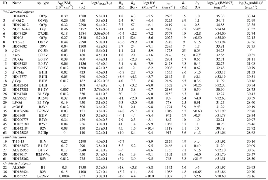
Table 1: ONLINE MATERIAL – List of targets, with their stellar and magnetic properties.
ID Name sp. type NH(ISM) d log(LBOL/L⊙) RA RK log( ˙M)a v∞ R∗ Bp log(LX)(B&M97) log(LX)(udd14)b
(1022cm−2) (pc) (R⊙) (R⊙) (M⊙yr−1) (km s−1) (R⊙) (G) (erg s−1) (erg s−1)
Well detected objects
1 HD148937 Of?p 0.39 1380 5.8±0.1 1.8 4.3 −5.5 2693 15 1.0 35.38 33.14 3 θ1Ori C O7Vfp 0.26 450 5.3±0.1 2.4 9.4 −6.4 3225 9.9 1.1 34.47 32.99 4 HD191612 Of?p 0.32 2290 5.4±0.2 3.7 57. −6.1 2119 14 2.5 34.85 33.35 5 NGC1624-2 O?p 0.46 5152 5.1±0.2 >11. 41. −6.8 2890 9.7 >20m >34.61 33.32 6 HD47129 O7.5III 0.18 1584 5.09±0.04 >5.4 <2.2 −7.2 3567 10 >2.8 >34.00 32.74 7 HD108 Of?p 0.27 2510 5.7±0.1 >1.7 526. −5.6 2022 19 >0.50 >35.00 32.13 8 Tr16-22 O8.5V 0.44 2290 5.0±0.1 >3.6 <9.9 −7.0 2742 9 >1.5 >33.94 32.56 9 HD57682 O9V 0.04 1300 4.8±0.2 3.7 24. −7.1 2395 7 1.7 33.81 32.35 10 ζOri O9.5Ib 0.05 414 5.6±0.1 1.1 2.1 −5.9 1723 25 0.06 34.25 c 11 τsco B0.2V 0.03 180 4.5±0.1 1.8 20. −7.6 2176 5.6 0.20m 32.85 30.35 12 NU Ori B0.5V 0.39 400 4.4±0.1 3.5 <2.3 −8.1 2901 5.7 0.65 32.71 31.11 13 HD63425 B0.5V 0.06 1136 4.5±0.4 3.1 <16. −7.9 2478 6.8 0.46 32.75 31.08 14 HD66665 B0.5V 0.012 1500 4.2±0.5 4.0 12. −8.2 2008 5.5 0.67 32.48 30.79 15 ξ1CMa B1III 0.02 423 4.6±0.1 >5.3 2.7 −7.5 1555 8.6 >1.5 >33.17 31.53 17 HD47777 B1III 0.05 760 4.0±0.2 >8.6 <4.3 −8.7 2142 5 >2.1 >32.19 30.51 18 βCep B1IV 0.017 182 4.22±0.08 4.0 7.3 −8.6 2169 6.5 0.36 31.99 30.16 20 HD122451 B1III 0 108 4.4±0.2 >3.1 <3.2 −8.0 1552 8.7 >0.25 >32.33 30.34 21 HD127381 B1-2V 0.007 127 3.76±0.06 7.5 3.8 −9.7 2186 4.8 0.50 30.90 28.73 26 HD64740 B1.5Vp 0.012 350 4.1±0.3 30. 1.9 −9.0 2152 6.3 16 32.27 30.43 28 ALS9522 B1.5Ve 0.32 1800 4.0±0.1 >11. <2.0 −8.0 989 6.4 >4.0 >32.63 30.59 29 LP Ori B1.5Vp 0.19 450 3.1±0.2 6.3 <3.0 −9.0 758 2.5 0.91 31.27 28.60 31 σOri E B2Vp 0.012 500 3.6±0.2 31. 2.1 −9.8 1794 3.9 9.6m 31.29 29.19 35 HD136504 B2IV-V 0.03 131 3.8±0.2 >4.8 <5.7 −8.3 1019 5.3 >0.60 >31.99 29.78 39 HD3360 B2IV 0.017 183 3.7±0.2 >4.1 4.4 −8.4 942 5.9 >0.34 >31.78 29.34 42 HD200775 B2Ve 0.34 429 4.0±0.3 7.9 2.3 −8.1 862 10 1.0 32.21 29.97 45 HD182180 B2Vn 0.04 236 3.0±0.1 41. 1.4 −9.9 1058 3.7 11. 30.93 28.46 47 HD142184 B2V 0.08 130 2.8±0.1 45. 1.6 −10.4 1118 3.1 10. 30.48 27.92 63 HD125823 B7IIIp 0 140 3.2±0.1 >10. 8.4 −9.4 917 3.6 >1.3 >31.06 28.68 Faint detections 19 Tr16-13 B1V 0.27 2290 4.0±0.1 >7.7 −8.9 2129 4.9 >1.4 >31.92 30.16 23 HD163472 B1-2V 0.17 290 3.8±0.1 5.2 5.2 −9.5 2466 4.1 0.40 31.20 29.09 27 ALS15956 B1.5V 0.17 5848 4.3±0.2 >9. −8.6 1755 9.1 >1.5 >32.10 30.36 30 HD37017 B2:IV-Vp 0.05 450 3.4±0.2 >18. 1.9 −9.1 1102 3.9 >6.0 >31.70 29.57 61 HD175362 B5V 0.012 275 3.2±0.1 >59. 3.0 −9.5 765 5.8 >21.m >31.31 28.50 Undetected objects 22 ALS3694 B1 0.3 1750 3.7±0.3 >18. <3.8 −8.8 1142 5.6 >6 >31.97 29.93 36 HD156424 B2V 0.15 1100 3.7±0.4 >5.2 <11. −8.5 1058 4.8 >0.65 >31.86 29.70 46 HD55522 B2IV-V 0.0004 257 3.0±0.1 >19. 4.4 −10.0 1037 3.3 >2.6 >30.60 28.16 2 0
Table 1: Continued
ID Name sp. type NH(ISM) d log(LBOL/L⊙) RA RK log( ˙M)a v∞ R∗ Bp log(LX)(B&M97) log(LX)(udd14)b
(1022cm−2) (pc) (R
⊙) (R⊙) (M⊙yr−1) (km s−1) (R⊙) (G) (erg s−1) (erg s−1)
49 HD36485 B3Vp 0.03 524 3.5±0.1 24. 2.4 −9.0 1012 4.5 10. 31.85 29.63
51 HD306795 B3V 0.1 2100 3.2±0.3 >21. <3.6 −9.3 821 4.1 >5.0 >31.31 28.81 56 HD37058 B3VpC 0.012 758 3.5±0.2 >16. 8.6 −9.0 822 5.6 >3.0 >31.54 29.13
Columns giving the ID, Name, sp. type, log(LBOL/L⊙), RA, RK, R∗and Bpare reproduced from Tables 1 and 6 of Petit et al. (2013). The distance d, mass-loss rates log( ˙M), and color excesses (used to calculate
the NH(ISM), see text) are the ones used in the Petit et al. paper: they were not extensively listed there and are thus reproduced here for completeness. In fact, distances d and reddening for stars with luminosity
determined by Petit et al. (2013) appear in their Table 4 and 5 while for the other objects, they were taken from the references in their Table 2. Mass-loss rates and wind velocities have been calculated using the recipes of Vink et al. (2000) for the chosen stellar parameters. Note that the ˙M corresponds to the mass driven from an equivalent unmagnetized star, which is the parameter used in theoretical models of MCWs. Discussions
on the errors of the stellar/magnetic parameters can be found in Petit et al. (2013, notably Sect. 3.3.3). Finally, the predictions log(LX)(B&M97) and log(LX)(udd14) listed in the last two columns were calculated using
the stellar/magnetic properties using the models of Babel & Montmerle (1997a) and ud-Doula et al. (2014), respectively (see also text for details). Notes: the dubious detection of ALS8988 is not mentioned.
aThe mass-loss rates correspond to those that the stars would have in absence of the field (which may not correspond to the actual mass-loss rate of the magnetic star, but are the parameters to be used in model
calculations).
bThese predictions have been calculated using the XADM model and a 10% efficiency. cThere is no prediction for this object as the wind of the star is not confined (η
∗<1).
mThere are higher multipoles components.
2
Table 2: ONLINE MATERIAL – List of targets, with the details of the X-ray observations. Note that, for XMM-Newton, the quoted exposure times correspond to the shortest amongst available EPIC cameras (usually pn).
ID Name X # Obs. ObsID (exp. time) ID Name X # Obs. ObsID (exp. time)
Well detected objects 12 NU Ori 4 XMM 0134531601 (16ks)
1 HD148937 1 XMM 0022140101 (10ks) 12 NU Ori 5 XMM 0134531701 (21ks)
1 HD148937 2 XMM 0022140601 (8ks) 12 NU Ori 6 Chandra 18 (47ks)
1 HD148937 3 Chandra 10982 (99ks) 12 NU Ori 7 Chandra 1522 (38ks) 3 θ1Ori C 1 XMM 0112590301 (37ks) 12 NU Ori 8 Chandra 3498 (69ks) 4 HD191612 1 XMM 0300600201 (9ks) 12 NU Ori 9 Chandra 3744 (164ks) 4 HD191612 2 XMM 0300600301 (12ks) 12 NU Ori 10 Chandra 4373 (171ks) 4 HD191612 3 XMM 0300600401 (24ks) 12 NU Ori 11 Chandra 4374 (169ks) 4 HD191612 4 XMM 0300600501 (11ks) 12 NU Ori 12 Chandra 4395 (100ks) 4 HD191612 5 XMM 0500680201 (19ks) 12 NU Ori 13 Chandra 4396 (165ks) 5 NGC1624-2 1 Chandra 14572 (49ks) 13 HD63425 1 XMM 0671990201 (18ks) 6 HD47129 1 XMM 0001730601 (14ks) 14 HD66665 1 XMM 0671990101 (25ks) 7 HD108 1 XMM 0109120101 (29ks) 15 ξ1CMa 1 XMM 0600530101 (7ks) 8 Tr16-22 1 XMM 0112560101 (23ks) 17 HD47777 1 XMM 0011420101 (31ks) 8 Tr16-22 2 XMM 0112560201 (24ks) 17 HD47777 2 XMM 0011420201 (34ks) 8 Tr16-22 3 XMM 0112560301 (29ks) 17 HD47777 3 Chandra 2540 (96ks) 8 Tr16-22 4 XMM 0112580601 (28ks) 17 HD47777 4 Chandra 13610 (92ks) 8 Tr16-22 5 XMM 0112580701 (8ks) 17 HD47777 5 Chandra 13611 (60ks) 8 Tr16-22 6 XMM 0145740101 (7ks) 17 HD47777 6 Chandra 14368 (74ks) 8 Tr16-22 7 XMM 0145740201 (7ks) 17 HD47777 7 Chandra 14369 (66ks) 8 Tr16-22 8 XMM 0145740301 (7ks) 18 βCep 1 XMM 0300490201 (28ks) 8 Tr16-22 9 XMM 0145740401 (8ks) 18 βCep 2 XMM 0300490301 (29ks) 8 Tr16-22 10 XMM 0145740501 (7ks) 18 βCep 3 XMM 0300490401 (28ks) 8 Tr16-22 11 XMM 0145780101 (8ks) 18 βCep 4 XMM 0300490501 (28ks) 8 Tr16-22 12 XMM 0160160101 (15ks) 20 HD122451 1 XMM 0150020101 (42ks) 8 Tr16-22 13 XMM 0160160901 (31ks) 21 HD127381 1 XMM 0690210101 (10ks) 8 Tr16-22 14 XMM 0160560101 (12ks) 26 HD64740 1 Chandra 13625 (15ks) 8 Tr16-22 15 XMM 0160560201 (12ks) 28 ALS9522 1 Chandra b
8 Tr16-22 16 XMM 0160560301 (19ks) 29 LP Ori 1 Chandra COUP (838ks) 8 Tr16-22 17 XMM 0311990101 (26ks) 31 σOri E 1 XMM 0101440301 (12ks) 8 Tr16-22 18 XMM 0560580101 (14ks) 31 σOri E 2 Chandra 3738 (91ks) 8 Tr16-22 19 XMM 0560580201 (11ks) 35 HD136504 1 XMM 0690210201 (5ks) 8 Tr16-22 20 XMM 0560580301 (26ks) 39 HD3360 1 XMM 0600530301 (14ks) 8 Tr16-22 21 XMM 0560580401 (23ks) 42 HD200775 1 XMM 0650320101 (9ks) 8 Tr16-22 22 XMM 0650840101 (27ks) 45 HD182180 1 XMM 0690210401 (8ks) 8 Tr16-22 23 Chandra 50 (12ks)a 47 HD142184 1 Chandra 13624 (26ks) 8 Tr16-22 24 Chandra 632 (90ks) 63 HD125823 1 Chandra 13618 (10ks) 8 Tr16-22 25 Chandra 1249 (10ks)a Faint detections
8 Tr16-22 26 Chandra 6402 (87ks) 19 Tr16-13 1 Chandra CCCP
8 Tr16-22 27 Chandra 11993 (44ks) 23 HD163472 1 XMM 0600530201 (9ks)
8 Tr16-22 28 Chandra 11994 (39ks) 27 ALS15956 1 Chandra CCCP
9 HD57682 1 XMM 0650320201 (8ks) 30 HD37017 1 XMM 0049560301 (14ks) 10 ζOri 1 XMM 0112530101 (40ks) 61 HD175362 1 Chandra 13619 (11ks) 10 ζOri 2 XMM 0657200101 (68ks) Undetected objects
10 ζOri 3 XMM 0657200201 (33ks) 22 ALS3694 1 Chandra 4503 (89ks) 10 ζOri 4 XMM 0657200301 (30ks) 36 HD156424 1 Chandra 5448 (20ks) 11 τsco 1 XMM 0112540101 (22ks) 46 HD55522 1 XMM 0690210301 (15ks) 12 NU Ori 1 XMM 0112590301 (38ks) 49 HD36485 1 Chandra 639 (49ks) 12 NU Ori 2 XMM 0093000101 (62ks) 51 HD306795 1 XMM 0201160401 (42ks)
Table 3: Luminosities (ISM absorption corrected, in the 0.5-10.0 keV band) and LX/LBOLratios for faint X-ray detec-tions of magnetic stars. Upper limits of the same quantities (90%) for non-detected objects.
ID Name sp. type LX log[LX/LBOL]
erg s−1 Faint detections 19 Tr16-13a B1V (6.5±3.4)e29 −7.8 ± 0.2 23 HD 163472 B1/2V (1.2±0.2)e29 −8.3 ± 0.1 27 ALS15956a B1.5V (1.5±0.5)e31 −6.7 ± 0.1 30 HD 37017 B1.5-2.5 IV-Vp (1.7±0.4)e29 −7.7 ± 0.1 61 HD 175362 B5V (7.3±3.4)e28 −7.9 ± 0.2 Non-detections 22 ALS3694 B1 <7.0e29 < −7.4 36 HD 156424 B2V <6.4e29 < −7.5 46 HD 55522 B2IV/V <2.6e28 < −8.1 49 HD 36485 B3Vp <5.0e28 < −8.3 51 HD 306795 B3V <4.2e29 < −7.1 56 HD 37058 B3VpC <1.0e29 < −8.0
Note:aFor Chandra observations of ALS15956 and Tr16-13, we used the X-ray luminosity derived in the Carina survey (Naz´e et al. 2012b), taking into account the