WASP-31b: a low-density planet transiting a metal-poor, late-F-type dwarf star

(1)

arXiv:1011.5882v1 [astro-ph.EP] 25 Nov 2010

Astronomy & Astrophysicsmanuscript no. wasp31 _{ESO 2010}c

November 30, 2010

WASP-31b: a low-density planet transiting a late-F-type star

⋆ , ⋆⋆

D. R. Anderson

1

, A. Collier Cameron

2

, C. Hellier

1

, M. Lendl

3

, T. A. Lister

4

, P. F. L. Maxted

1

, D. Queloz

3

,

B. Smalley

1

, A. M. S. Smith

1

, A. H. M. J. Triaud

3

, R. G. West

5

, D. J. A. Brown

2

, M. Gillon

6

, F. Pepe

3

, D. Pollacco

7

,

D. S´egransan

3

, R. A. Street

4

, and S. Udry

3 1 _{Astrophysics Group, Keele University, Staffordshire ST5 5BG, UK}

e-mail: dra@astro.keele.ac.uk

2 _{SUPA, School of Physics and Astronomy, University of St. Andrews, North Haugh, Fife KY16 9SS, UK} 3 _{Observatoire de Genève, Université de Genève, 51 Chemin des Maillettes, 1290 Sauverny, Switzerland} 4 _{Las Cumbres Observatory, 6740 Cortona Dr. Suite 102, Santa Barbara, CA 93117, USA}

5 _{Department of Physics and Astronomy, University of Leicester, Leicester LE1 7RH, UK}

6 _{Institut d’Astrophysique et de Géophysique, Université de Liège, Allée du 6 Août, 17, Bat. B5C, Liège 1, Belgium}

7 _{Astrophysics Research Centre, School of Mathematics & Physics, Queen’s University, University Road, Belfast BT7 1NN, UK}

Received February 9, 2099; accepted March 10, 2099

ABSTRACT

We report the discovery of the low-density, transiting giant planet WASP-31b. The planet is 0.47 Jupiter masses and 1.56 Jupiter radii. It is in a 3.4-day orbit around a .1-Gyr-old, late-F-type, V = 11.7 star, which is a member of a common proper motion pair. In terms of its low density, WASP-31b is second only to WASP-17b, which is a more highly irradiated planet of similar mass.

Key words.binaries: eclipsing – planetary systems – stars: individual: WASP-31

1. Introduction

To date, 107 transiting extrasolar planets have been discovered1, the majority of which are gas giants in short orbits. The radii of a subset of these exoplanets are larger than predicted by stan-dard models of irradiated gas giants (e.g., Burrows et al. 2007; Fortney et al. 2007), including TrES-4b (Mandushev et al. 2007; Sozzetti et al. 2009), 12b (Hebb et al. 2009), and WASP-17b (Anderson et al. 2010a,c). A number of mechanisms have been proposed as potential solutions to the radius anomaly (see Fortney et al. (2009) for a review), each of which involves either injecting heat into the planet from an external source or slowing heat loss from the planet.

One such mechanism is the dissipation of energy within a planet as heat during the tidal circularisation of an eccentric orbit (Bodenheimer et al. 2001; Gu et al. 2003; Jackson et al. 2008; Ibgui & Burrows 2009). Though these studies found that tidal heating would be sufficient to explain the large radii of even the most bloated exoplanets (although we would have to be observing some systems at very special times), they all trun-cated the tidal evolution equations to second order in eccen-tricity. Leconte et al. (2010) recently showed that, other than for near-circular orbits, one must solve the complete tidal equations. Neglecting to do so results in an underestimate of the energy dis-sipation rate and an overestimate of the timescale over which

en-⋆ _{Based in part on observations made with the HARPS}

spectro-graph on the 3.6-m ESO telescope (proposal 085.C-0393) and with the CORALIE spectrograph and the Euler camera on the 1.2-m Euler Swiss telescope, both at the ESO La Silla Observatory, Chile.

⋆⋆ _{The photometric time-series and radial velocity data used in}

this work are only available in electronic form at the CDS via anonymous ftp to cdsarc.u-strasbg.fr (130.79.128.5) or via http://cdsweb.u-strasbg.fr/cgi-bin/qcat?J/A+A/

1 _{2010 Nov 25, http://exoplanet.eu}

ergy is dissipated. The consequence is that tidal dissipation can account for the radii of moderately bloated planets, but not the most bloated ones.

Burrows et al. (2007) suggested that enhanced opacities would retard the loss of internal heat and thus slow contraction. These enhanced opacities were implemented by the use of su-persolar metallicities, a simplistic approach which neglects the increase in molecular weight that would partially or completely counter the effect on the planet radius (Guillot 2008). Also, strongly irradiated planetary atmospheres are radiative down to deep levels, so heavy elements are likely to settle out. However, atmospheric dynamics may keep the atmosphere well mixed (Showman et al. 2008; Spiegel et al. 2009).

The bloated planets are all very strongly irradiated by their host stars, and a small fraction of stellar insolation energy would be sufficient to account for the observed degrees of bloating. Guillot & Showman (2002) suggested that the kinetic energy of strong winds, induced in the atmosphere by the large day-night temperature contrasts that result from tidal locking, may be transported downward and deposited as thermal energy in the deep interior. However, a mechanism to convert the kinetic en-ergy into thermal enen-ergy would still be required. Li & Goodman (2010) and Youdin & Mitchell (2010) found that turbulence is efficient at dissipating kinetic energy. Magnetic drag on weakly ionized winds (Perna et al. 2010) and Ohmic heating (Batygin & Stevenson 2010) are alternative mechanisms. The non-bloated planets too are highly irradiated. Hence, either such a mechanism would either have to act more efficiently on the bloated planets, or some other property must counteract its ef-fect. One such possibility is the presence of a massive core. Indeed, Guillot et al. (2006) and Burrows et al. (2007) found a correlation between the core masses required to reproduce the

(2)

Fig. 1. WASP-South discovery light curve. Upper panel:

Photometry folded on the orbital period of P = 3.4 d. Points with error above three times the median error (0.012 mag) were clipped for display purposes. Lower panel: Photometry folded on the orbital period and binned in phase (∆φ = 0.025), with the transit model generated from the parameters of Table 2 superim-posed.

observed radii of known exoplanets and the metallicities of their host stars.

In this paper, we present the discovery of the bloated, tran-siting, giant planet WASP-31b. Compared to the ensemble of known short-period planets, WASP-31b is moderately irradiated by its low-metallicity host star.

2. Observations

WASP-31 is a V = 11.7, F7–8 star located in the constel-lation Crater. WASP-31 has been observed by WASP-South (Pollacco et al. 2006) during the first five months of each year since the start of full-scale operations (2006 May 4), and four of these five seasons of data were available at the time of writ-ing. A transit search (Collier Cameron et al. 2006) of the result-ing 19 815 usable photometric measurements (Figure 1) found a strong, 3.4-d periodicity.

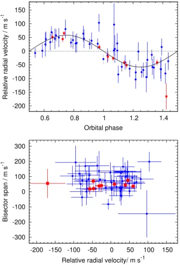
Using the CORALIE spectrograph mounted on the 1.2-m Euler-Swiss telescope (Baranne et al. 1996; Queloz et al. 2000b), we obtained 34 spectra of WASP-31 during 2009 and a further 13 spectra during 2010. In April 2010, we obtained an additional 10 spectra with the HARPS spectrograph mounted on the 3.6-m ESO telescope. Radial velocity (RV) measurements were computed by weighted cross-correlation (Baranne et al. 1996; Pepe et al. 2005) with a numerical G2-spectral template. RV variations were detected with the same period found from the WASP photometry and with a semi-amplitude of 58 m s−1, consistent with a planetary-mass companion. The RV measure-mentsvare plotted in Figure 2.

To test the hypothesis that the RV variations are due to spectral line distortions caused by a blended eclipsing binary, a line-bisector analysis (Queloz et al. 2001) of the CORALIE and HARPS cross-correlation functions was performed. The lack of correlation between bisector span and RV (Figure 2, lower panel), especially for the high-precision HARPS measurements, supports the identification of the transiting body as a planet.

Fig. 2. Upper panel: Spectroscopic orbit of WASP-30, as

illus-trated by CORALIE (blue circles) and HARPS (red squares) ra-dial velocities. The best-fitting Keplerian model, generated from the parameters of Table 2, is overplotted as a solid line. An RV taken at BJD = 2 455 168.8468, depicted in the plot with dotted error bars, fell during transit. As we did not treat the Rossiter-McLaughlin effect (e.g., Queloz et al. 2000a), we ex-cluded this measurement from our combined analysis. Lower

panel: A lack of correlation between bisector spans and radial

velocities rules out a blended eclipsing binary or starspots as the cause of the photometric and spectroscopic variaitions. We adopted uncertainties on the bisector spans twice the size of those on the radial velocities. For both plots, the centre-of-mass velocity, γ = −125 m s−1_{, was subtracted from the radial} veloc-ities and the Keplerian model.

To refine the system paramters, we obtained high signal-to-noise transit photometry. Photometric follow-up observations of WASP-31 were obtained with the LCOGT2 _{2.0-m Faulkes}

Telescope North (FTN) on Mt. Haleakala, Maui on the night of 2010 Feb 26. The fs03 Spectral Instruments camera was used with a 2 × 2 binning mode giving a field of view of 10′× 10′and a pixel scale of 0.303 arcsec/pixel. The data were taken through a Pan-STARRS-z filter and the telescope was defocussed to pre-vent saturation and to allow 60-sec exposure times to be used.

The data were pre-processed using the WASP Pipeline (Pollacco et al. 2006) to perform masterbias and flat construc-tion, debiassing and flatfielding. Due to the very low dark cur-rent of the fs03 Fairchild CCD (< 0.0001 e−_{/pix/sec), dark}

(3)

Fig. 3. High signal-to-noise transit light curves. The upper

ob-servations (blue circles) were obtained by FTN, using a Pan-STARRS z filter, on 2010 Feb 26. The lower observations (red diamonds), offset in relative flux by 0.026 for display, were ob-tained by Euler, using a Gunn r filter, on 2010 Apr 15. The best-fitting transit models generated from the parameters of Table 2 are overplotted.

traction was not performed. Aperture photometry was performed using DAOPHOT within the IRAF environment using an aper-ture with a radius of 11 pixels. Differential photometry was then performed relative to 20 comparison stars that were within the FTN field of view (Figure 3).

On 2010 April 15 we obtained 4.1 hours of photometry in the Gunn r filter with the Euler camera on the Euler-Swiss telescope, covering a complete transit together with 40 and 55 minutes of observations before and after the transit, respectively. The con-ditions were variable, with seeing ranging from 0.6 arcsec to 1.7 arcsec while an airmass range of 1.15 to 1.34 was covered. Euler now employs absolute tracking to keep the stars on the same pix-els during a whole transit. By identifying point sources in each image and matching them with a catalogue, the image centre is calculated. Drifts from the nominal position are then corrected by adjusting the telescope pointing between exposures.

After bias-subtracting and flat-fielding the images, we per-formed aperture photometry. The flux was extracted for all stars in the field and the final light curve (Figure 3) was obtained by differential photometry of the target and a reference source ob-tained by combining the 4 brightest reference stars. The aver-age accuracy obtained was 2.7 mmag, which was limited by the number of available reference stars.

Table 1. Stellar parameters from the spectroscopic analysis

Parameter Value T_∗,eff _{6300 ± 100 K} log g_∗ _{4.4 ± 0.1 (cgs)} ξt 1.4 ± 0.1 km s−1 v sin i _{7.6 ± 0.4 km s}−1 [Fe/H] −0.20 ± 0.09 [Na/H] −0.24 ± 0.04 [Mg/H] −0.11 ± 0.06 [Si/H] −0.13 ± 0.07 [Ca/H] −0.03 ± 0.08 [Sc/H] −0.07 ± 0.06 [Ti/H] −0.10 ± 0.09 [V/H] _{−0.16 ± 0.09} [Cr/H] _{−0.20 ± 0.08} [Mn/H] _{−0.45 ± 0.11} [Ni/H] −0.25 ± 0.08 log A(Li)[LTE] _{2.82 ± 0.08} log A(Li)[NLTE] _{2.75 ± 0.08} M_∗ _{1.15 ± 0.08 M}_⊙ R_∗ _{1.12 ± 0.15 M}_⊙ R.A. (J2000) = 11h₁₇m_45.35s Dec. (J2000) = −19◦₀₃′_17.3′′ USNO-B1.0 0709-0239208 2MASS 11174536-1903171

Note: NLTE Lithium value using correction of Carlsson et al. (1994).

Mass and Radius estimate using the Torres et al. (2010) calibration.

3. Stellar parameters

The individual HARPS spectra of WASP-31 were co-added to produce a single spectrum with an average S/N of around 100:1. The analysis was performed using the methods given in Gillon et al. (2009). The Hα line was used to determine the ef-fective temperature (T_∗,eff), while the Na i D and Mg i b lines were used as surface gravity (log g_∗) diagnostics. The parame-ters obtained from the analysis are listed in Table 1. The elemen-tal abundances were determined from equivalent width measure-ments of several clean and unblended lines. A value for micro-turbulence (ξt) was determined from Fe i using the method of

Magain (1984). The quoted error estimates include that given by the uncertainties in T_∗,eff, log g_∗and ξt, as well as the scatter due

to measurement and atomic data uncertainties.

The projected stellar rotation velocity (v sin i) was deter-mined by fitting the profiles of several unblended Fe i lines. We assumed a value for macroturbulence (vmac) of 5.2 ± 0.3 km s−1,

based on the tabulation by Gray (2008), and we used an instru-mental FWHM of 0.06 ± 0.01 Å, determined from the telluric lines around 6300Å. A best-fitting value of v sin i = 7.6 ± 0.4 km s−1was obtained. However, recent work by Bruntt et al. (2010) suggests a lower value for macroturbulence of vmac = 4.2 ± 0.3

km s−1 _{which yields a slightly higher v sin i = 8.1 ± 0.4 km} s−1_{. We therefore adopt the average of these two determinations,} v sin i = 7.9 ± 0.6 km s−1_{. If v}

mac= 0 km s−1, then a value of

v sin i = 8.7 ± 0.4 km s−1_{is found, which is the upper-limit of} the projected rotation velocity.

4. Combined analysis

The WASP, FTN and Euler photometry were combined with the CORALIE and HARPS radial velocities in a si-multaneous Markov-chain Monte Carlo (MCMC) analysis (Collier Cameron et al. 2007; Pollacco et al. 2008; Enoch et al. 2010b). The proposal parameters we used are: Tc, P, ∆F, T14, b,

(4)

K1, T∗,eff, [Fe/H], √e cos ω and √e sin ω. Here Tcis the epoch

of mid-transit, P is the orbital period, ∆F = Rp2/R∗2is the frac-tional flux-deficit that would be observed during transit in the absence of limb-darkening, T14is the total transit duration (from

first to fourth contact), b is the impact parameter of the planet’s path across the stellar disc, K1is the stellar reflex velocity

semi-amplitude, T_∗,effis the stellar effective temperature, [Fe/H] is the stellar metallicity, e is the orbital eccentricity and ω is the argu-ment of periastron.

As Ford (2006) notes, it is convenient to use e cos ω and e sin ω as MCMC jump parameters, because these two quantities are nearly orthogonal and their joint probability density function is well-behaved when the eccentricity is small and ω is highly uncertain. Ford cautions, however, that the use of e cos ω and e sin ω as jump parameters implicitly imposes a prior on the ec-centricity that increases linearly with e. Instead we use √e cos ω and √e sin ω as jump parameters, which restores a uniform prior on e.

At each step in the MCMC procedure, each proposal pa-rameter is perturbed from its previous value by a small, ran-dom amount. From the proposal parameters, model light and RV curves are generated and χ2 _{is calculated from their}

compari-son with the data. A step is accepted if χ2(our merit function) is lower than for the previous step; a step with higher χ2_{is accepted}

with probability exp(−∆χ2_/_{2). In this way, the parameter space}

around the optimum solution is thoroughly explored. The value and uncertainty for each parameter are respectively taken as the median and central 68.3% confidence interval of the parameter’s marginalised posterior probability distribution. At each step in the MCMC procedure, we calculate the centre-of-mass velocity, γ, at the fiducial epoch of transit as the mean of the RV residu-lals about the RV model. We do this separately for the CORALIE and HARPS data, to allow for a systematic instrumental offset, ∆γHARPS, between the two spectrographs.

From the proposal parameters, we calculate the mass M, radius R, density ρ, and surface gravity log g of both the star (which we denote with subscript *) and the planet (which we denote with subscript P), as well as the equilibrium temperature of the planet TP,eqlassuming it to be a black-body and that energy

is efficiently redistributed from the planet’s day-side to its night-side. We also calculate the transit ingress and egress durations, T12and T34, and the orbital semi-major axis a.

With eccentricity floating, we find e = 0.027+0.034

−0.020. Applying the ‘F-test’ of Lucy & Sweeney (1971), we find a 66% proba-bility that an eccentricity of or above the fitted value could have arisen by chance if the the underlying orbit is in fact circular. As such, we impose a circular orbit, but we note that doing so has no signicant effect as the fitted eccentricity was so small.

The median parameter values and their 1-σ uncertainties from our MCMC analysis are presented in the middle column of Table 2. The corresponding best-fitting transit light curves are shown in Figure 1 and Figure 3, and the best-fitting RV curve is shown in Figure 2.

Without exquisite photometry, our implentation of MCMC tends to bias the impact parameter, and thus R_∗and RP, to higher

values. This is because, with low signal-to-noise photometry, the transit ingress and egress durations are uncertain, and symmet-ric uncertainties in those translate into asymmetsymmet-ric uncertain-ties in b and thus in R_∗. The effect on the stellar and planetary radii is larger for high-impact-parameter planets such as WASP-31b. Therefore we explored an MCMC with a main-sequence (MS) prior imposed (Collier Cameron et al. 2007). This employs a Bayesian penalty to ensure that, in accepted steps, the values of stellar radius are consistent with the values of stellar mass for

Table 2. System parameters from the combined analysis

Parameter (Unit) no MS prior with MS prior

(adopted solution) P (d) _{3.405909 ± 0.000005} _{3.405909 ± 0.000005} Tc(HJD-2450000) 5189.2828 ± 0.0003 5189.2828 ± 0.0003 T14(d) 0.1107 ± 0.0014 0.1093 ± 0.0012 T12= T34(d) 0.0276 ± 0.0020 0.0257 ± 0.0016 ∆F = R2 P/R 2 ∗ 0.01622 ± 0.00032 0.01596 ± 0.00029 b _{0.769 ± 0.016} _{0.752 ± 0.016} i (◦₎ _{84.54 ± 0.27} _{84.81 ± 0.23} K1(m s−1) 58.2 ± 3.5 58.0 ± 3.5 a (AU) _{0.04657 ± 0.00034} _{0.04662 ± 0.00035} e 0 (adopted) 0 (adopted) γCORALIE(m s−1) −124.924 ± 0.036 −124.922 ± 0.036 ∆γHARPS(m s−1) −5.268 ± 0.096 −5.264 ± 0.096 M_∗(M_⊙) _{1.161 ± 0.026} _{1.165 ± 0.026} R_∗(R_⊙) _{1.241 ± 0.039} _{1.206 ± 0.035} ρ_∗(ρ_⊙) _{0.608 ± 0.052} _{0.664 ± 0.050} log g_∗(cgs) _{4.316 ± 0.024} _{4.341 ± 0.021} T_∗,eff(K) _{6203 ± 98} _{6339 ± 99} [Fe/H] −0.19 ± 0.09 −0.18 ± 0.09 MP(MJup) 0.478 ± 0.030 0.477 ± 0.030 RP(RJup) 1.537 ± 0.060 1.482 ± 0.053 ρP(ρJup) 0.132 ± 0.017 0.146 ± 0.017 log gP(cgs) 2.665 ± 0.042 2.696 ± 0.038 TP,eql(K) 1568 ± 33 1555 ± 33

Table 3. Proper motions of WASP-31 and its visual companion

Star Catalogue µRA(mas) µDec(mas)

WASP-31 UCAC3 −28.2 ± 1.3 −0.4 ± 1.6

WASP-31 PPXML −25.0 ± 2.3 −0.1 ± 2.4

Companion UCAC3 _{−33.1 ± 3.1} _{+1.0 ± 3.8} Companion PPXML _{−28.5 ± 4.2} _{+1.6 ± 4.2}

a main-sequence star. The difference between the solutions with and without MS priors is small (Table 2), indicating that the tran-sit light curves are of a quality such that the ingress and egress durations are measured sufficiently well. As such, we adopt the solution without the MS prior, which has more conservative er-ror bars.

5. System age

WASP-31 is a visual double with a V ∼ 15.8 star (2MASS 11174477-1903521) approximately 35′′ _away3_{. The 2MASS}

colours of the companion suggest that it is a mid-to-late K-type star. The proper motions for the two stars listed in the PPMXL (Roeser et al. 2010) and UCAC3 (Zacharias et al. 2010) catalogues suggest that this is a common proper motion pair (Table 3).

Using 2MASS photometry we constructed a colour-magnitude diagram (Figure 4). A distance modulus of 8.0 ± 0.2 (400 ± 40 pc) is required to place the companion on the main-sequence, and this puts WASP-31 very close to the zero-age 3 _{The companion is blended with WASP-31 in the WASP images.}

Though it is 40 times fainter than WASP-31 and it is resolved in the Euler and FTN images, we did correct the WASP photometry for the contamination prior to producing the MCMC solution presented. We checked the effect of the contamination by producing another MCMC solution using the non-corrected WASP photometry. The best-fitting pa-rameter values were the same to within a tenth of an error bar.

(5)

Fig. 4. Colour-magnitude diagram for WASP-31 and its

compan-ion. Various isochrones from Marigo et al. (2008) are given, with ages indicated in the figure.

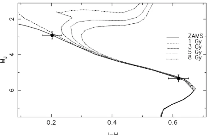
Fig. 5. Modified H-R diagram. The evolutionary mass tracks

(Z = 0.017 ≈ [Fe/H] = −0.05; Y = 0.30) and isochrones (Z = 0.012 ≈ [Fe/H] = −0.20) for the ages 0.5, 1, 2, 3, 4, 5 and 10 Gyr are from Marigo et al. (2008).

main sequence and 1-Gyr age lines. At a distance of 400 pc, the two stars would be separated by at least 14 000 AU (0.2 light-year).

Assuming aligned stellar-spin and planetary-orbit axes, the measured v sin i of WASP-31 and its derived stellar radius indi-cate a rotational period of Prot = 8.0 ± 0.7 d. Combining this

with the B − V colour of an an F6 star from Gray (2008), we used the relationship of Barnes (2007) to estimate a gyrochrono-logical age of 1.5+1.3

−0.6Gyr. We found no evidence for rotational modulation in the WASP light curves.

The lithium abundance (ALi= 2.75±0.10) found in WASP-31

implies an age (Sestito & Randich 2005) between that of open clusters such as M34 (250 Myr; ALi= 2.92 ± 0.13) and NGC 752

(2 Gyr; ALi= 2.65 ± 0.13). However, lithium is a poor indicator

of age for a star as hot as WASP-31, and the measured abundance is consistent at the 1-σ level with that of the upper envelope of the 5-Gyr M67 (ALi= 2.55 ± 0.18).

We interpolated the stellar evolution tracks of Marigo et al. (2008) using ρ_∗ from the MCMC analysis and using T_∗,eff and [Fe/H] from the spectral analysis (Figure 5). This suggests an age of 4 ± 1 Gyr and a mass of 1.12 ± 0.05 M⊙for WASP-31.

6. Discussion

With a mass of 0.48 MJup and a radius of 1.54 RJup,

WASP-31b has a density 13 per cent that of Jupiter and is ∼0.3 RJup

larger than predicted by standard models of irradiated gas giants (Fortney et al. 2007). Only WASP-17b (Anderson et al. 2010a), which has a similar mass (0.49 MJup), is known to have a lower

density (0.06 ρJup, Anderson et al. 2010c).

With an increasingly large sample of well-characterised planets, we can begin to make statistical inferences as to the physical reasons behind their diverse natures. Enoch et al. (2010a) showed the radii of 16 of the 18 known low-mass (0.1– 0.6 MJup) planets strongly correlate with equilibrium

temper-ature and host-star metallicity. The calibration of Enoch et al. (2010a) predicts a radius of 1.39 RJup for WASP-31b. In a

similar study, but using a different metallicity dependence and treating the 74 known Jupiter-mass (0.2–2.5 MJup) planets,

Anderson et al. (2010b) also found a strong correlation be-tween planetary radius and equilibrium temperature and host-star metallicity. The calibration of Anderson et al. (2010b) pre-dicts a radius of 1.23 RJupfor WASP-31b. In each case, the

pre-dicted radius of WASP-31b is smaller than the measured radius (1.54 ± 0.06 RJup).

WASP-31 has a similarly low metallicity to WASP-17 ([Fe/H] = −0.19 ± 0.09; Triaud et al. 2010), thus both could rea-sonably be expected to have small cores (Guillot et al. 2006; Burrows et al. 2007). However, this would only somewhat ex-plain why the two planets are so large. Both planets are highly irradiated, with 17b being more irradiated than WASP-31b as, despite being in a slightly wider orbit (a = 0.052 AU), its host star is larger (R_∗ = 1.58 R_⊙) and hotter (T_∗,eff = 6650 K; Anderson et al. 2010c). This results in an equilibrium tem-perature for WASP-17b hotter by 200 K than for WASP-31b and, from this, we could expect WASP-17b to be larger than WASP-31b. Both planets, though, are larger than predicted by standard models of irradiated giant planets (e.g. Fortney et al. 2007), and by the empirical relations of Enoch et al. (2010a) and Anderson et al. (2010b). Hence, it seems likely that some addi-tional physics is at play.

The RV data place a stringent upper limit on WASP-31b’s or-bital eccentricity (e < 0.13; 3σ). It is therefore unlikely that tidal heating resulting from the circularisation of an eccentric orbit (e.g. Bodenheimer et al. 2001) was responsible for significantly inflating the planet. However, we could happen to be viewing the system soon after circularisation occurred and prior to the planet significantly contracting. This would have made finding the planet easier due to the greater transit depth.

The metallicity of WASP-31 is at the lower end of what may be expected for a star of its age in the Solar neighbourhood (at a Galactocentric radius of 8.5 kpc; Magrini et al. 2009).

Acknowledgements. WASP-South is hosted by the South African Astronomical

Observatory and we are grateful for their ongoing support and assistance. Funding for WASP comes from consortium universities and from the UK’s Science and Technology Facilities Council. M. Gillon acknowledges support from the Belgian Science Policy Office in the form of a Return Grant.

References

Anderson, D. R., Hellier, C., Gillon, M., et al. 2010a, ApJ, 709, 159 Anderson, D. R. et al. 2010b, in preparation

Anderson, D. R. et al. 2010c, in preparation

Baranne, A., Queloz, D., Mayor, M., et al. 1996, A&AS, 119, 373 Barnes, S. A. 2007, ApJ, 669, 1167

Batygin, K. & Stevenson, D. J. 2010, ApJ, 714, L238

Bodenheimer, P., Lin, D. N. C., & Mardling, R. A. 2001, ApJ, 548, 466 Bruntt, H., Bedding, T. R., Quirion, P., et al. 2010, MNRAS, 405, 1907

(6)

Burrows, A., Hubeny, I., Budaj, J., & Hubbard, W. B. 2007, ApJ, 661, 502 Carlsson, M., Rutten, R. J., Bruls, J. H. M. J., & Shchukina, N. G. 1994, A&A,

288, 860

Collier Cameron, A., Pollacco, D., Street, R. A., et al. 2006, MNRAS, 373, 799 Collier Cameron, A., Wilson, D. M., West, R. G., et al. 2007, MNRAS, 380,

1230

Enoch, B., Cameron, A. C., Anderson, D. R., et al. 2010a, MNRAS, 1531 Enoch, B., Collier Cameron, A., Parley, N. R., & Hebb, L. 2010b, A&A, 516,

A33+

Ford, E. B. 2006, ApJ, 642, 505

Fortney, J. J., Baraffe, I., & Militzer, B. 2009, ArXiv e-prints Fortney, J. J., Marley, M. S., & Barnes, J. W. 2007, ApJ, 659, 1661 Gillon, M., Smalley, B., Hebb, L., et al. 2009, A&A, 496, 259

Gray, D. F. 2008, The Observation and Analysis of Stellar Photospheres, ed. Gray, D. F.

Gu, P., Lin, D. N. C., & Bodenheimer, P. H. 2003, ApJ, 588, 509 Guillot, T. 2008, Physica Scripta Volume T, 130, 014023 Guillot, T., Santos, N. C., Pont, F., et al. 2006, A&A, 453, L21 Guillot, T. & Showman, A. P. 2002, A&A, 385, 156

Hebb, L., Collier-Cameron, A., Loeillet, B., et al. 2009, ApJ, 693, 1920 Ibgui, L. & Burrows, A. 2009, ApJ, 700, 1921

Jackson, B., Greenberg, R., & Barnes, R. 2008, ApJ, 681, 1631

Leconte, J., Chabrier, G., Baraffe, I., & Levrard, B. 2010, A&A, 516, A64+ Li, J. & Goodman, J. 2010, ArXiv e-prints

Lucy, L. B. & Sweeney, M. A. 1971, AJ, 76, 544 Magain, P. 1984, A&A, 134, 189

Magrini, L., Sestito, P., Randich, S., & Galli, D. 2009, A&A, 494, 95

Mandushev, G., O’Donovan, F. T., Charbonneau, D., et al. 2007, ApJ, 667, L195 Marigo, P., Girardi, L., Bressan, A., et al. 2008, A&A, 482, 883

Pepe, F., Mayor, M., Queloz, D., et al. 2005, The Messenger, 120, 22 Perna, R., Menou, K., & Rauscher, E. 2010, ApJ, 719, 1421

Pollacco, D., Skillen, I., Collier Cameron, A., et al. 2008, MNRAS, 385, 1576 Pollacco, D. L., Skillen, I., Cameron, A. C., et al. 2006, PASP, 118, 1407 Queloz, D., Eggenberger, A., Mayor, M., et al. 2000a, A&A, 359, L13 Queloz, D., Henry, G. W., Sivan, J. P., et al. 2001, A&A, 379, 279 Queloz, D., Mayor, M., Weber, L., et al. 2000b, A&A, 354, 99 Roeser, S., Demleitner, M., & Schilbach, E. 2010, AJ, 139, 2440 Sestito, P. & Randich, S. 2005, A&A, 442, 615

Showman, A. P., Menou, K., & Cho, J. 2008, in Astronomical Society of the Pacific Conference Series, Vol. 398, Astronomical Society of the Pacific Conference Series, ed. D. Fischer, F. A. Rasio, S. E. Thorsett, & A. Wolszczan, 419–+

Sozzetti, A., Torres, G., Charbonneau, D., et al. 2009, ApJ, 691, 1145 Spiegel, D. S., Silverio, K., & Burrows, A. 2009, ApJ, 699, 1487 Torres, G., Andersen, J., & Gim´enez, A. 2010, A&A Rev., 18, 67

Triaud, A. H. M. J., Collier Cameron, A., Queloz, D., et al. 2010, ArXiv e-prints Youdin, A. N. & Mitchell, J. L. 2010, ApJ, 721, 1113