Development of an integrated modelling framework for evaluating beneficial management practices Phase I: Hydrologic modelling in Bras d'Henri Watershed (BH), Quebec, and development of the GIBSI integrated, economic-hydrologic, modelling system

(1)

Development of an integrated

modelling framework for

evaluating beneficial management

practices

Phase I

(2)

(3)

Hydrologie Modelling in Bras d'Henri Watershed (BH),

Quebee, and Development of the GIBSI Integrated,

Economie-Hydrologie, Modelling System

2006/2007 Ducks Unlimited Canada (DUC) WEBs Progress Report

Alain N. Rousseau, Ph.D., ing. Stéphane Savary, M.Sc..

Renaud Quilbé, D.Se. Sébastien Tremblay

Centre Eau Terre et Environnement

Institut national de la recherche scientifique (INRS-ETE) 490, rue de la Couronne, Québec (QC), G lK 9A9

Report N° R910

(4)

(5)

LIST OF FIGURES

Figure 1. DEM of the Beaurivage watershed... 15 Figure 2. Stream network of the Beaurivage watershed... 16 Figure 3. Comparison of the modelled path-flow directions using Orlandini’s algortihm

(i,j,k,l) and other algortihms such as the D8-LAD & D8-LTD methods (e,f,g,h) for four synthetic drainage systems (a,b,c,d) (Orlandini et al., 2003)... 17

Figure 4. Flow directions of Beaurivage watershed and main outlet surrounding cell... 18 Figure 5. Comparison of the current Beaurivage watershed boundary based on the

20-m DEM (black line) with that generated using the 100-20-m resolution DEM (as depicted by the green area) ... 18

Figure 6. Current (a) and previous (b) Beaurivage river network generated using

PHYSITEL... 20

Figure 7. Current (a) and previous (b) BH river network generated using PHYSITEL... 20 Figure 8. Current (a) and previous (b) computational domains of RHHUs of the

Beaurivage watershed... 21

Figure 9. Current (a) and previous (b) computational domains of RHHU of the BH

watershed... 21

Figure 10. 1995 land use classes of the Beaurivage watershed... 22 Figure 11. Soil polygon map of the Beaurivage watershed ... 24 Figure 12. Example of the determination of the weighted mean soil type and properties

for a RHHU ... 24

Figure 13. Current (a) and previous (b) mean soil types of Beaurivage watershed

RHHUs ... 25

Figure 14. Mean soil properties difference between previous and current Beaurivage

(8)

Figure 15. Current Beaurivage watershed project within HYDROTEL ...27 Figure 16. Current (a) and previous (b) simulated and measured streamflows for

calibration of HYDROTEL on Beaurivage watershed for the 1984-1985 hydrological year. ...29

Figure 17. Current (a) and previous (b) simulated and measured streamflows for

calibration of HYDROTEL on Beaurivage watershed for the 1988-1989 hydrological year. ...29

validation of HYDROTEL on Beaurivage watershed for hydrological year 1990-1991...30

Figure 19.Current (a) and previous (b) simulated and measured streamflows for

validation of HYDROTEL on Beaurivage watershed for hydrological year 1992-1993...31

(9)

LIST OT TABLES

Table 1. Land use occupation of the Beaurivage and BH watersheds ... 23

Table 2. HYDROTEL submodel simulation options... 28

Table 3. Comparison of HYDROTEL performance for the calibration period... 30

Table 4. Comparison of HYDROTEL performance for the validation period... 31

Table 5. Comparison of HYDROTEL long term behaviour (1994-1994) ... 32

(10)

(11)

A. RATIONALE FOR INTEGRATED MODELLING WORK

Within the Bras d’Henri (BH) watershed, Quebec, farmers and councillor members of ‘Club de fertilization de la Beauce’ have been implementing Beneficial Management Practices (BMPs) such as riparian buffers, reduced herbicide use, hog slurry management and crop rotation. Water quality impacts of these BMPs are being monitored and recorded at the outlets of studied micro-watershed and the BH watershed. These efforts established a solid foundation for developing an integrated modelling framework to examine economic and environmental tradeoffs of BMPs and to evaluate cost effectiveness of conservation projects in these watersheds. The knowledge developed in the proposed study will make a contribution to the Watershed Evaluation of BMPs (WEBs project; AAFC, 2006b), a national initiative led by the Agricultural and Agri-Food Canada (AAFC) and Ducks Unlimited Canada (DUC), and will have important policy implications for better design of agricultural conservation programs within the Agricultural Policy Framework of AAFC (AAFC, 2006a).

B. OBJECTIVES AND HYPOTHESES

The purpose of the modelling component of WEBs is to develop an integrated modelling framework for evaluating economic and environmental outcomes of BMPs in agricultural watersheds (see Yang et al. (2007): “An Integrated Economic-Hydrologic Modelling Framework for the Watershed Evaluation of Beneficial Management Practices: A Conceptual Framework”). In the proposed project, we are leading the development of a prototype, integrated, economic-hydrological, modelling system based on the Canadian Integrated Modelling System (IMS) GIBSI (‘Gestion Intégrée des Bassins Versants à l’aide d’un Système Informatisé’), developed by INRS-ETE (Mailhot et al., 1997; Villeneuve et al., 1998; Rousseau et al., 2000; 2005a). In this modelling system for BH watershed, the hydrologic model will be integrated with the on-farm economic model(s) and the farm behaviour model(s) (developed under separate agreements with other Bruno LaRue of Université Laval, Paul Thomassin of McGill University, and Peter Boxall of University of Alberta). The modelling system will be further developed if non-market valuation model(s) are available in the subsequent phase. The Phase I of this project has the following objectives:

(i) To apply a hydrologic model (GIBSI) to characterize water quality benefits of BMPs within the BH watershed; and

(12)

(ii) To develop a prototype, integrated modelling system based on GIBSI to examine the economic and environmental tradeoffs of BMPs within BH.

C. METHODS

C.1. To apply hydrologic model to characterize water quality benefits of bmps

The purpose of hydrologic modelling is to characterize watershed processes under base conditions and examine water quality benefits of BMP implementation. For this project, the integrated, economic-hydrological, modelling system GIBSI will be used to accomplish this task. GIBSI is comprised of a database, simulation models (hydrology, soil erosion, agricultural-chemical transport, and water quality), management modules (land use, point source, agricultural production systems, and reservoir management modules), a relational database management system and a geographic information system (GIS). The database includes readily available spatial and attribute data and decision variables which can be used to compare simulation results with water quality standards. The computational units (i.e., spatial simulation unit or SSU) used in GIBSI consist of elementary sub-watersheds (also referred to as relatively homogenous hydrological units). The computational time step is the day. The agricultural management module of GIBSI allows for the modification of management parameters of one or more SSUs, sub-watersheds of the main water courses or administrative units (e.g., municipality).

Basic input data for the hydrologic model may be derived from the following datasets: climate data, Digital Elevation Model (DEM) data, land use data, soil data, hydrographic and hydrometric data. Climate data like precipitation and temperature represent the driving forces of the hydrologic processes. The DEM data, in conjunction with river network data, set up the spatial structure and surface runoff routing of the watershed. The DEM data also provide data for important model parameters such as slope, slope length, and aspect (flow direction). The land use data including agricultural management practices is the basis for defining crop-related model parameters such as crop type, crop rotation, tillage, crop management factor, and conservation practice factor. Other than those input data, stream flow data and water quality data will be used for model calibration and validation. Because GIBSI uses sub-watersheds as computational units and some BMPs such as riparian buffers are located along the hydrographic network, the model will need to be adapted to adequately model the impact of these popular alternative management practices. One possible way to resolve this problem is to link a field-scale model of riparian buffers such as Riparian Ecosystem System model (REMM) (Lowrance et al., 2000) with the watershed model (e.g., Yang and Weersink, 2004).

(13)

The current application of GIBSI focuses on the BH watershed, a sub-watershed (150 km2_{) of}

the Beaurivage River watershed (727 km2_{), the latter being a sub-watershed of the Chaudière}

River watershed (6682 km2_{). Several applications of GIBSI have taken place on the Chaudière}

River watershed. For example, Mailhot et al. (2002), Lavigne et al. (2004), Rousseau et al. (2002), and Salvano et al. (2004, 2006) respectively used GIBSI to: (i) quantify the impacts of a municipal clean water program on the water quality of this watershed, (ii) predict the impact of deforestation on the hydrologic regime of the 728-km2_{Famine River watershed, another}

sub-watershed of the Chaudière, (iii) develop a risk-based TMDL (total maximum daily load) assessment approach, and (iv) illustrate the importance of valuing environmental benefits associated with water quality improvement in the assessment of mandatory nutrient management plans required by Quebec legislation.

In the application of Salvano et al. (2004, 2006), two scenarios were considered: (i) a base-case scenario assuming application of all available manure and (ii) an on-farm nutrient management scenario based on meeting phosphorus crop requirements with manure and treating any manure surpluses. Two types of management units were selected to evaluate these scenarios: (i) contiguous municipalities, and (ii) watersheds. Results showed that management at sub-watershed levels had the largest environmental benefit/on-farm cost (B/C) ratio when compared to contiguous municipalities. For one of those sub-watersheds, the ratio was close to one although only various recreational benefits were accounted for in the calculation. If a more holistic set of benefits would have been accounted for, a B/C ratio greater than one would surely have been obtained. A sensitivity analysis revealed that variations of 37.5%, 22.5%, and - 20% for monetary benefits, on-farm manure treatment costs, and average probabilities of exceeding the targeted water quality standard were necessary to obtain a B/C ratio greater than one, respectively. Such a framework provides a means to compare regulation, policy and agricultural BMP scenarios and identifies the most suitable scenario in terms of monetary value of environmental benefits resulting from water quality improvements (i.e., benefits of restored water uses) and on-farm costs (i.e., costs of manure treatment technologies). One of the characteristics of this B/C analysis methodology relates to the flexibility of data management. Data updates can be easily carried out either directly by modifying the data in the database or at the time of analysis using the graphical user interface (GUI) of GIBSI. This way, it becomes possible to directly verify the impact of various BMP parameters on the B/C ratio.

For all the above applications, the Chaudière watershed was subdivided into 1849 SSUs (i.e., relatively homogeneous hydrological units, RHHUs) averaging 350 ha. Within the Bras d’Henri watershed, the BMPs are being implemented on 900-ha micro-watersheds and water quality impacts of these BMPs are being monitored and recorded at the outlets of the micro-watershed and the BH micro-watershed. To meet the specific needs of this project, GIBSI needs to

(14)

be implemented at the scale of the Beaurivage River watershed (727 km2_{) in order to have}

RHHUs between 50 to 100 ha on average. This application will provide a means to examine the impacts of the studied BMPs of the BH micro-watersheds studied by AAFC at various up scaling levels, that is, those of the BH and Beaurivage River watersheds.

C.2. To develop a prototype IMS to examine economic and environmental tradeoffs of BMPs

In the proposed project, we will lead the development of a prototype, integrated, economic-hydrological, modelling system based on GIBSI. In this modelling system for BH, the hydrologic model will be integrated with the on-farm economic model(s) and the farm behaviour model(s) (developed under separate agreements as mentioned before). As mentioned before, on-farm economics and farm behavioural model(s) for BH are being developed in part by Bruno La Rue of Université Laval and Paul Thomassin of McGill University. These models will be eventually integrated in GIBSI for BH. The modelling system will be further developed if non-market valuation model(s) are available in the subsequent phase of WEBs I.

The IMS will have several important features. First, it will serve as a data management tool for various models (i.e., watershed information system). The GUI will be used to assemble various datasets together and develop data protocols. In particular, economic data associated with farm production or BMP adoption will be managed using the GUI to facilitate model integration. This will be particularly important given the spatial distribution of multiple farm operations in the watershed. Second, the framework will build GIS functions to manipulate those datasets to establish common spatial references. For example, economic data collection is based on farm field boundary or the boundaries defined by the fields owned or rented by various farm managers, but the hydrologic data may be based on sub-watershed boundaries or smaller units. Overlaying, re-sampling or aggregating can be used to establish common spatial units for various datasets. Third, visualization tools will be developed to view data with 2-D maps, figures, and tables to examine spatial patterns of economic and environmental characteristics in the study sites. Fourth, data analysis tools could be developed to examine the tradeoffs between on-farm economic costs and environmental improvements in study sites under different BMP adoption scenarios. For example, spatial patterns of high costs and high benefits, high costs and low benefits, low costs and high benefits, and low costs and low benefits could be generated to illustrate economic and environmental tradeoffs within study watersheds.

(15)

D. COMPLETED MILESTONES AND ACTIVITIES

As mentioned before, the BH watershed (150 km2₎ _{is located within the Chaudière River}

watershed (6682 km2_{) so we can say that the model is running on the study site using RHHUs}

of about 350 ha. To meet the specific requirements of this project, GIBSI needs to have RHHUs between 50 to 100 ha on average. Such downscaling process requires a complete reintegration of the Beaurivage watershed into the spatial and attribute database of GIBSI. To accomplish this task, the following steps need to be performed:

(i) Definition of the spatial structure and surface runoff routing of the Beaurivage watershed using PHYSITEL (Turcotte et al., 2001; Royer et al., 2006; Rousseau et al., 2007).

(ii) Calibration of the hydrological model of GIBSI, that is HYDROTEL (Fortin et al., 2001a,b), on the Beaurivage watershed.

(iii) Updating of the existing GIBSI database, simulation models, and relational database management system structure to characterize water quality benefits of BMPs within the BH watershed.

D.1. Completed from October 1, 2006 – December 31, 2006

D1.1. Collection and preparation of input data for GIBSI:

(i) The spatial structure and surface runoff routing of the Beaurivage watershed are completely redefined at a higher resolution to support precise physical representation of the BH watershed application. The RHHUs (100 ha) were defined using PHYSITEL which includes the newly integrated path-based algorithm of Orlandini et al. (2003) for the determination of non dispersive drainage directions in grid-based DEM. When compared to the aforementioned applications of GIBSI on the Chaudière River watershed. The downscaling process was supported by a higher resolution DEM and a more precise digitized river network.

(ii) The discretized Beaurivage watershed was successfully integrated into HYDROTEL and the calibration of the model has been undertaken.

(16)

D.1.2. Projected activities from January 1, 2007 to March 31, 2007 include:

(i) Completion of the hydrologic calibration of HYDROTEL on the Beaurivage watershed and comparison of simulated and measured streamflows at the outlet of the BH watershed.

(ii) Updating of the GIBSI database, simulation models, and relational database management system structure to characterize water quality benefits of BMPs within the BH watershed.

E. PLANNED ACTIVITIES FOR 2007/08

(i) Run GIBSI for selected BMPs and supply environmental export coefficients (i.e., mass of agricultural contaminants/cropland/period of Interest).

(ii) Design the integration of on-farm economic model(s) developed by Bruno LaRue of Université Laval and Paul Thomassin of McGill University in the integrated modelling system.

F. PRELIMINARY RESULTS

Preliminary results mainly refer to the presentation of the completed tasks (construction of the watershed database using PHYSITEL; calibration of HYDROTEL on the Beaurivage watershed) and comparison to previous applications on the Chaudière river watershed with emphasis on the simulation of stream flows.

F.1. Construction of the Beaurivage watershed database using PHYSITEL

PHYSITEL is a watershed GIS developed to determine the topographical, path-flow structure to support hydrological modelling using HYDROTEL. To determine the path-flow structure, PHYSITEL requires as input data: a DEM and a digitized river network. Also, as required by HYDROTEL, land use and soil type data need to be integrated into PHYSITEL to complete the physiographic characterisation of each RHHU.

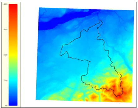
For this project, we used a high-resolution (20 m) DEM of the Beaurivage watershed. This resolution captures the essential topographic features of the watershed in order to reflect the

(17)

spatial variability of the hydrologic response of the watershed. Previous applications of GIBSI on the Chaudière watershed were based on a lower-resolution DEM (100 m) that limited the representation of the topography and the accurate discretization of the Beaurivage watershed, river network, and sub-watersheds such as the BH watershed. A higher-resolution DEM allows for an improved simulation of the hydrological response of small watersheds such as those of the Beaurivage and BH. The DEM data provide the basic information to derive the slope, slope length, and flow direction of and within RHHUs.

Figure 1 presents the DEM of the Beaurivage watershed (represented here by approximate watershed boundary). Note that the illustrated watershed boundary is that approximated from the previous application of PHYSITEL using the 100-m DEM of the watershed. This display allows for a global localisation of the Beaurivage watershed.

Figure 1. DEM of the Beaurivage watershed

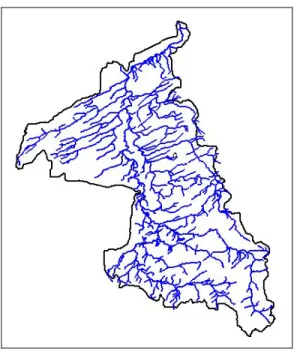
The high-resolution stream network and the watershed path-flow structure have improved the identification of lakes, reservoirs and ponds which could not be detected by DEM analysis solely. Also, definition of the RHHUs can be influenced by stream network complexity and ramification. Consequently, the BH watershed river network can be reproduced or represented either with a small or a large group of streams that restrain or increase the definition of

(18)

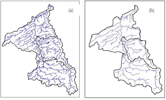
RHHUs and the implementation of BMPs. Figure 2 presents the stream network of the Beaurivage watershed with the previous watershed boundary.

Figure 2. Stream network of the Beaurivage watershed

The next step required by PHYSITEL calls for the determination of the modified altitude values of the stream network and within a buffer zone along the network. This stream burning process simplifies the water drainage and path-flow structure from land surface to stream. Based on the DEM, PHYSITEL calculates the slope of every pixel composing the DEM matrix. Note that the slopes are defined with north-south and east-west couples of neighbouring altitudes.

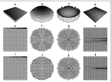
The modified altitudes and slopes are used for the determination of flow directions according to the Orlandini algorithm (Orlandini et al., 2003). We have shown that this algorithm is superior to other algorithms based on computational time and physical representation of path-flow path-flow directions (Rousseau et al., 2005b). This performance relates to the determination of a cumulative (path-based) deviation matrix that influences downstream, cell-flow direction by considering upstream, cell-flow direction. Figure 3 presents a comparison of the performance of Orlandini’s algorithm with other algorithms with respect to the accuracy of the modelled drainage network of four synthetic drainage systems.

(19)

Figure 3. Comparison of the modelled path-flow directions using Orlandini’s algortihm

(i,j,k,l) and other algortihms such as the D8-LAD & D8-LTD methods (e,f,g,h) for four synthetic drainage systems (a,b,c,d) (Orlandini et al., 2003).

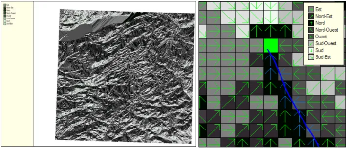
These results show that Orlandini’s cumulative (path-based) deviation matrix allows for the reasonably accurate reproductions of flow directions that are non-locally unbiased with respect to grid orientation. Thus, Orlandini’s algorithm will contribute to the improved physical representation of computational sub-watersheds (RHHUs) based on cell-to-cell upstream processes. Figure 4 presents the flow directions of the Beaurivage watershed and its outlet. Once the main outlet of the watershed is defined, PHYSITEL identifies all surrounding cells flowing into the main outlet and, going upstream from cell-to-cell, all the cells constituting the watershed. The resulting watershed boundary can be redefined via edition of flow directions to insure appropriate superposition of land use data and watershed area. This process prevents the accounting of null land use area over the watershed. Figure 5 compares the current Beaurivage watershed boundary with that generated using the 100-m resolution DEM.

(20)

Figure 4. Flow directions of Beaurivage watershed and main outlet surrounding cell.

Figure 5. Comparison of the current Beaurivage watershed boundary based on the 20-m

DEM (black line) with that generated using the 100-m resolution DEM (as depicted by the green area)

(21)

Figure 5 shows notable differences between the current and previous Beaurivage delimitations. They can be attributed to the following points:

• The previous PHYSITEL application was based on the use of a 100-m DEM and D8 method to determine the path-flow structure that limited the precision of the watershed definition. Lower resolution may interfere with determination of flow directions leading to inaccurate cell rejection or consideration in the watershed constituting algorithm.

• Globally, in both instances the drainage area remains similar but the use of a high-resolution DEM suggests better representation of the watershed physical boundaries.

Since the drainage identification process determines implicitly and inherently the internal drainage structure of the watershed, the next step consists inidentifying the river network by assuming that all cells draining more than a specific upstream area are part of that network. A more or less detailed river network can be identified, depending on the selected upstream threshold area. This step is crucial for the delineation of RHHUs. A small upstream threshold area will result in a detailed river network associated with a complex distribution of RHHUs. On the other hand, a high upstream threshold area will result in a simplifed river network and distribution of RHHUs. The previous application of PHYSITEL on the Chaudière watershed resulted in a simplified representation of the Beaurivage river network leading to a limited number of RHHUs composing the watershed. The same observation occurs for the BH watershed. The current application produces a detailed river network with better representation of the integrated stream network. Consequently, stream network ramification resulted into a larger numbers of RHHUs over both the Beaurivage and BH watersheds. Figures 6 and 7 respectively present the and previous Beaurivage and BH river networks generated using PHYSITEL. Also Figure 6 includes both Beaurivage and BH watershed boundaries.

(22)

Figure 6. Current (a) and previous (b) Beaurivage river network generated using PHYSITEL

Figure 7. Current (a) and previous (b) BH river network generated using PHYSITEL

Both previous river networks clearly demonstrate that the current application on Beaurivage watershed produces a detailed river network. Ensuing network ramifications with respect to the original stream network (Figure 2) have resulted into a high-resolution computational domain of RHHUs. Increased number and improved resolution of RHHUs will be conducive to more precise BMPs applications with increased physical representation of land surface path-flow structure.

(b) (a)

(23)

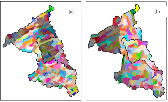
The resulting computational domain of RHHUs corresponds to the segmentation of the studied watersheds into stream-associated land area. Thus, every RHHU is associated to a single river segment. Figures 8 and 9 present current and previous computational domains of RHHUs of the Beaurivage and BH watersheds, respectively.

Figure 8. Current (a) and previous (b) computational domains of RHHUs of the Beaurivage

watershed

Figure 9. Current (a) and previous (b) computational domains of RHHU of the BH

watershed

Figures 8 and 9 show the current application is more detailed with an important diminution in the average size of RHHUs. Newly defined RHHUs are in agreement with the downscaling study objectives and allow for a more precise definition of BMPs. Note that the previous application was characterized by 192 RHHUs (mean area of 375 ha) for the Beaurivage

(a) (b)

(24)

watershed (Figure 8b) and 30 RHHUs (mean area of 440 ha) for the Bras d’Henri watershed (Figure 9b). The current application regroups 675 RHHUs (mean area of 105 ha) for the Beaurivage watershed (Figure 8a) and 127 RHHUs (mean area of 120 ha) for the Bras d’Henri watershed (Figure 9a). The large number of RHHUs is needed for improving the simulation of the water quality in any part of the Beaurivage or BH watershed.

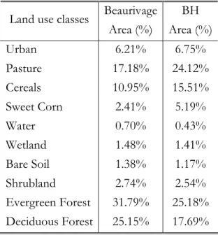
To complete the watershed description for hydrologic simulation, land use classes and soil types are defined for the entire Beaurivage watershed. The previous application required land use determination of the Chaudière watershed. This land use determination was derived from processing a Landsat TM image taken on August 28, 1995 (Gauthier et al., 1996). To compare with the previous hydrologic simulation, the same land use classification map was reused. This map presents the distinctive classes required by GIBSI. Note that recent work on land use evolution of Chaudière watershed generated land use maps for different years (1976, 1981, 1987, 1990, 1995, 1999, 2003) (Savary et al., 2006). These maps were derived using a continuous object-oriented classification process of Lansat images. Identified classes for every scenario also respected GIBSI’s classes. Figure 10 presents the 1995 land use classification map of the Beaurivage watershed. Table 1 introduces the percentages of each land use classes of the studied watersheds (Beaurivage and BH).

(25)

Table 1. Land use occupation of the Beaurivage and BH watersheds

Beaurivage BH Land use classes

Area (%) Area (%) Urban 6.21% 6.75% Pasture 17.18% 24.12% Cereals 10.95% 15.51% Sweet Corn 2.41% 5.19% Water 0.70% 0.43% Wetland 1.48% 1.41% Bare Soil 1.38% 1.17% Shrubland 2.74% 2.54% Evergreen Forest 31.79% 25.18% Deciduous Forest 25.15% 17.69%

Table 1 shows that both watersheds are mainly covered by agricultural land (Pasture, Cereals and Sweet Corn) and forest land (Shrubland, Evergreen Forest, Deciduous Forest). Globally, the area of the Beaurivage watershed is made of agricultural land (30%) and forest land (60%). Also, the BH watershed is characterized by intensively cultivated area (45% the area). In both watersheds, the remaining 10% of the total area is covered by other classes such urban, bare soil and shrubland.

Finally, PHYSITEL requires the integration of soil types for each RHHUs. Mean soil types are determined from soil information provided by soil maps for each cell constituting the watershed. Note that in the current version of HYDROTEL, hydraulic characteristics of those soil types are considered vertically constant. Default values from Rawls and Brakensiek (1989) are available in the model, but the user can substitute any other more appropriate values for them. In the present case, soil types for Beaurivage watershed are described by soil polygons (Figure 11). Each soil polygon is also characterised by physico-chemical properties as required by GIBSI and HYDROTEL. As hydraulic characteristics are needed for each RHHUs, superposition of the RHHU (Figure 8a) and soil polygon maps allows for computation of weighted mean soil physico-chemical properties based on underlying soil polygons and associated soil information. Note that the colours of the soil type map are note associated with any specific physico-chemical properties, they are randomly selected to facilitate display.

(26)

Figure 11. Soil polygon map of the Beaurivage watershed

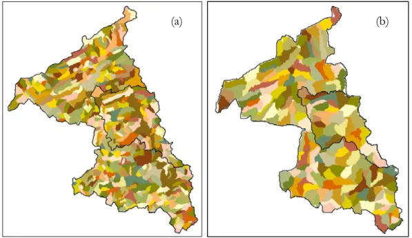
Figure 12 illustrates the weighted mean calculation procedure for each soil type and associated physico-chemical properties for a RHHU. Previous and current soil characterisations refer to the same weighted mean calculation process for each RHHU’s soil physico-chemical properties. Consequently, current soil definition of the Beaurivage watershed RHHUs (Figure 13a) can be compared with the previous application (Figure 13b).

Figure 12. Example of the determination of the weighted mean soil type and properties for a

RHHU

Weighted mean soil type and physico-chemical properties process

(27)

Figure 13. Current (a) and previous (b) mean soil types of Beaurivage watershed RHHUs

To compare current and previous RHHU soil type definition, spatial mean difference of soil physico-chemical properties can be calculated for the common area covered by each RHHU of both applications. Figure 14 presents the mean difference between previous and current soil properties.

(28)

Figure 14. Mean soil properties difference between previous and current Beaurivage watershed application

Figure 14 illustrates that current and previous physico-chemical properties present notable differences. More precisely, the mean difference between previous and current RHHU soil properties is less than 25% for 60% of the Beaurivage common watershed area and less then 50% for 80% of the common area. Such differences between soil physico-chemical properties mainly relate to watershed RHHU spatial definition as the current application presents an increased number of RHHUs with higher resolution.

The soil type and properties definition completes the watershed integration using PHYSITEL.

F.2. Calibration of HYDROTEL on the Beaurivage watershed

Since the hydrological model of GIBSI is HYDROTEL, the current application requires calibration of the model on the Beaurivage watershed. Following the PHYSITEL application, the Beaurivage was successfully integrated into HYDROTEL. The calibration is based on the comparison of simulated and measured streamflows. The previous calibration results showed good agreement between simulated and measured streamflows. Similarly, the current hydrologic calibration was successfully achieved.

(29)

HYDROTEL is a distributed hydrological model compatible with remote sensing and GIS. All the model’s input data files are generated using PHYSITEL. In addition, HYDROTEL requires meteorological and hydrometric data files. These files include measurements at the meteorological and streamflow stations. Existing files for the previous Chaudière watershed application can be reused for the current Beaurivage watershed application. Figure 15 presents the current Beaurivage watershed project within HYDROTEL.

Note that the hydrologic simulations are supported by seven meteorological stations covering the Beaurivage watershed area. Also, two gauging stations located at the outlets of the Beaurivage and BH will be used for comparison between measured and simulated streamflows.

Figure 15. Current Beaurivage watershed project within HYDROTEL

Simulations with the HYDROTEL model are based on a modular approach in order to facilitate the modification of the content of any module as well as the addition of new ones. As shown in table 2, each submodel generally offers more than one simulation option. These options have been selected so that the model could be applied on any watershed, given the available meteorological data. Simulation can be obtained either for daily time steps or for time steps that are submultiples of 24 hours, depending on the watershed, on the specific objectives of the simulation and on the available data. Note that current and previous submodel options are bold in table 2.

(30)

Current calibration of model parameters were performed using simulated and measured streamflows for the 1984-1989 hydrological years (October of year i to September of year i+1), for Beaurivage watershed at Saint-Étienne (upstream of watershed main outlet). Current results are from an optimized set of model parameters that are identical for all RHHUs over the whole watershed. Temporal validation of the calibration was performed using the 1989-1994 hydrological years. Long-term model behaviour was also assessed for the calibration and validation periods. Current calibration of HYDROTEL can also be compared to the previous application results.

Table 2. HYDROTEL submodel simulation options

Submodel Options Estimation of meteorological varaibles Thiessen polygons

Weighted mean of nearest three stations

Accumulation and melt of snowpack Mixed (degree-day) energy-budget method

Potential evapotranspiration Thornthwaite

Linacre

Penman-Monteith Priestley-Taylor

Hydro-Québec

Vertical water budget BV3C

Surface and subsurface flow on each watershed Kinematic wave equation

Channel routing Kinematic wave equation

Diffusive wave equation

Figures 16 and 17 show examples of calibration results for the 1984-1985 and 1988-1989 hydrological years, respectively. Also, table 3 presents model performance for the complete calibration period based on the Nash-Sutcliffe criterion. Figure 16 and 17 show that measured streamflows are simulated quite satisfactorily in both current and previous applications. Nonetheless, discrepancies between simulated and measured streamflows occur particularly for the snow melting period.

(31)

Figure 16. Current (a) and previous (b) simulated and measured streamflows for calibration of

HYDROTEL on Beaurivage watershed for the 1984-1985 hydrological year.

calibration of HYDROTEL on Beaurivage watershed for the 1988-1989 hydrological year.

HYDROTEL has a tendency to underestimate the spring peak flow. Also, some events are not simulated at all and this is most likely due missing meteorological data or undetected precipitation events. 0 50 100 150 200 250 1 984-10 -0 1 1 984-10 -1 5 1 984-10 -2 9 1 984-11 -1 2 1 984-11 -2 6 1 984-12 -1 0 1 984-12 -2 4 1 985-01 -0 7 1 985-01 -2 1 1 985-02 -0 4 1 985-02 -1 8 1 985-03 -0 4 1 985-03 -1 8 1 985-04 -0 1 1 985-04 -1 5 1 985-04 -2 9 1 985-05 -1 3 1 985-05 -2 7 1 985-06 -1 0 1 985-06 -2 4 1 985-07 -0 8 1 985-07 -2 2 1 985-08 -0 5 1 985-08 -1 9 1 985-09 -0 2 1 985-09 -1 6 1 985-09 -3 0 Date St re am fl o w (m 3/s ) Measured Calculated 0 50 100 150 200 250 1 984-10 -0 1 1 984-10 -1 5 1 984-10 -2 9 1 984-11 -1 2 1 984-11 -2 6 1 984-12 -1 0 1 984-12 -2 4 1 985-01 -0 7 1 985-01 -2 1 1 985-02 -0 4 1 985-02 -1 8 1 985-03 -0 4 1 985-03 -1 8 1 985-04 -0 1 1 985-04 -1 5 1 985-04 -2 9 1 985-05 -1 3 1 985-05 -2 7 1 985-06 -1 0 1 985-06 -2 4 1 985-07 -0 8 1 985-07 -2 2 1 985-08 -0 5 1 985-08 -1 9 1 985-09 -0 2 1 985-09 -1 6 1 985-09 -3 0 Date St re am fl o w (m 3/s ) Measured Calculated (a) (b) 0 50 100 150 200 250 19 88- 10-01 19 88- 10-15 19 88- 10-29 19 88- 11-12 19 88- 11-26 19 88- 12-10 19 88- 12-24 19 89- 01-07 19 89- 01-21 19 89- 02-04 19 89- 02-18 19 89- 03-04 19 89- 03-18 19 89- 04-01 19 89- 04-15 19 89- 04-29 19 89- 05-13 19 89- 05-27 19 89- 06-10 19 89- 06-24 19 89- 07-08 19 89- 07-22 19 89- 08-05 19 89- 08-19 19 89- 09-02 19 89- 09-16 19 89- 09-30 Date S tr ea m fl o w (m 3/s ) Measured Calculated 0 50 100 150 200 250 19 88- 10-01 19 88- 10-15 19 88- 10-29 19 88- 11-12 19 88- 11-26 19 88- 12-10 19 88- 12-24 19 89- 01-07 19 89- 01-21 19 89- 02-04 19 89- 02-18 19 89- 03-04 19 89- 03-18 19 89- 04-01 19 89- 04-15 19 89- 04-29 19 89- 05-13 19 89- 05-27 19 89- 06-10 19 89- 06-24 19 89- 07-08 19 89- 07-22 19 89- 08-05 19 89- 08-19 19 89- 09-02 19 89- 09-16 19 89- 09-30 Date S tr ea m fl o w (m 3/s ) Measured Calculated (a) (b)

(32)

Table 3. Comparison of HYDROTEL performance for the calibration period

Calibration period (Hydrological years / October 1st_{to September 30}th₎

Nash-Sutcliffe 1984-1985 1985-1986 1986-1987 1987-1988 1988-1989 Total

Current 0.84 0.69 0.74 0.73 0.73 0.74

Previous 0.84 0.80 0.52 0.79 0.73 0.75

Figures 16 and 17 and table 3 demonstrate that the current calibration shows similar results to previous application. Year-to-year variation and accuracy can be attributed to the high-resolution watershed database obtained using PHYSITEL, peak flow synchronisation, winter streamflow measurements and erroneous meteorological data or missing meteorological events.

Figures 18 and 19 introduce examples of validation results for the 1990-1991 and 1992-1993 hydrological years. Also, table 4 presents HYDROTEL model performance for the complete validation period based on the Nash-Sutcliffe criterion.

Figure 18. Current (a) and previous (b) simulated and measured streamflows for validation

of HYDROTEL on Beaurivage watershed for hydrological year 1990-1991

0 50 100 150 200 250 19 91-10 -0 1 19 91-10 -1 5 19 91-10 -2 9 19 91-11 -1 2 19 91-11 -2 6 19 91-12 -1 0 19 91-12 -2 4 19 92-01 -0 7 19 92-01 -2 1 19 92-02 -0 4 19 92-02 -1 8 19 92-03 -0 3 19 92-03 -1 7 19 92-03 -3 1 19 92-04 -1 4 19 92-04 -2 8 19 92-05 -1 2 19 92-05 -2 6 19 92-06 -0 9 19 92-06 -2 3 19 92-07 -0 7 19 92-07 -2 1 19 92-08 -0 4 19 92-08 -1 8 19 92-09 -0 1 19 92-09 -1 5 19 92-09 -2 9 Date Str ea m fl o w (m 3/s ) Measured Calculated 0 50 100 150 200 250 19 91-10 -0 1 19 91-10 -1 5 19 91-10 -2 9 19 91-11 -1 2 19 91-11 -2 6 19 91-12 -1 0 19 91-12 -2 4 19 92-01 -0 7 19 92-01 -2 1 19 92-02 -0 4 19 92-02 -1 8 19 92-03 -0 3 19 92-03 -1 7 19 92-03 -3 1 19 92-04 -1 4 19 92-04 -2 8 19 92-05 -1 2 19 92-05 -2 6 19 92-06 -0 9 19 92-06 -2 3 19 92-07 -0 7 19 92-07 -2 1 19 92-08 -0 4 19 92-08 -1 8 19 92-09 -0 1 19 92-09 -1 5 19 92-09 -2 9 Date Str ea m fl o w (m 3/s ) Measured Calculated _(a) _(b)

(33)

Figure 19. Current (a) and previous (b) simulated and measured streamflows for validation of

HYDROTEL on Beaurivage watershed for hydrological year 1992-1993.

Figures 18 and 19 show relatively good agreement in steamflow simulations compare to calibration period. However, note that the spring peak flow is underestimated and that some individual flow events are missing.

Table 4. Comparison of HYDROTEL performance for the validation period

Validation period (Hydrological years / October 1th to September 30th) Nash-Sutcliffe 1989-1990 1990-1991 1991-1992 1992-1993 1993-1994 Total

Current 0.51 0.69 0.65 0.82 0.82 0.73

Previous 0.74 0.84 0.78 0.56 0.79 0.74

Figures 18 and 19 and table 4 demonstrate that the current validation shows similar results to the previous application for precise hydrological years and the cumulative calibration period. Again, year-to-year variation and accuracy can be attributed to the high-resolution watershed database obtained using PHYSITEL, peak flow synchronisation, winter streamflow measurements and erroneous meteorological data or missing meteorological events.

Finally, table 5 presents a comparison between current and previous long term HYDROTEL model behaviour for the 1984-1994 period.

0 50 100 150 200 250 19 92-10 -0 1 19 92-10 -1 5 19 92-10 -2 9 19 92-11 -1 2 19 92-11 -2 6 19 92-12 -1 0 19 92-12 -2 4 19 93-01 -0 7 19 93-01 -2 1 19 93-02 -0 4 19 93-02 -1 8 19 93-03 -0 4 19 93-03 -1 8 19 93-04 -0 1 19 93-04 -1 5 19 93-04 -2 9 19 93-05 -1 3 19 93-05 -2 7 19 93-06 -1 0 19 93-06 -2 4 19 93-07 -0 8 19 93-07 -2 2 19 93-08 -0 5 19 93-08 -1 9 19 93-09 -0 2 19 93-09 -1 6 19 93-09 -3 0 Date S treamf lo w ( m 3/s ) Measured Calculated 0 50 100 150 200 250 19 92-10 -0 1 19 92-10 -1 5 19 92-10 -2 9 19 92-11 -1 2 19 92-11 -2 6 19 92-12 -1 0 19 92-12 -2 4 19 93-01 -0 7 19 93-01 -2 1 19 93-02 -0 4 19 93-02 -1 8 19 93-03 -0 4 19 93-03 -1 8 19 93-04 -0 1 19 93-04 -1 5 19 93-04 -2 9 19 93-05 -1 3 19 93-05 -2 7 19 93-06 -1 0 19 93-06 -2 4 19 93-07 -0 8 19 93-07 -2 2 19 93-08 -0 5 19 93-08 -1 9 19 93-09 -0 2 19 93-09 -1 6 19 93-09 -3 0 Date S treamf lo w ( m 3/s ) Measured Calculated (a) (b)

(34)

Table 5. Comparison of HYDROTEL long term behaviour (1994-1994)

Current Calibration Previous Calibration

Correlation Coefficient 0.74 0.74

Nash-Sutcliffe Criterion 0.73 0.74

Measured runoff [mm] 617 617

Simulated runoff [mm] 558 551

Table 5 shows satisfying and comparable long term HYDROTEL performance for current and previous calibration. Nevertheless, the model has a tendency to underestimate the measured values at the Beaurivage outlet. This underestimation is most likely due to lower accuracy of streamflow measurements under ice cover. We can thus say that the hydrologic calibration exercise of the Beaurivage watershed has been successfully undertaken with repect to the objective of evaluating the impact of BMPs on water quality.

Additional efforts will be deployed to perform the hydrologic calibration of the BH watershed based on comparison of simulated and measured streamflows. The previous calibration did not include a comparison between simulated and measured streamflows at the outlet of the BH watershed. Recently acquired streamflow measurements will allow such comparison and will be used to refine the hydrologic calibration on the study area.

In summary, the current hydrologic modelling of the Beaurivage watershed offers a more detailed and appropriate representation of the watershed spatial variability. Such benefits meet the needs of the project since the downscaling process resulted in RHHUs with mean area of 105 ha.

G. DISCUSSION

Current integration of the Beaurivage watershed using PHYSITEL and hydrologic calibration of HYDROTEL model represent the principal achievements of the project activities for year 2006-2007 (actually, October 1st_{through January 31}st_).1_{These two major steps required the}

1_{Appendix I introduces the PowerPoint presentation on the Progress Report, Development of the GIBSI}

Integrated, Economic-Hydrologic, Modelling System for the Beaurivage/Bras d’Henri Watershed, that we made at the WEBs 3rd_{Annual Technical Workshop, February 7-8, 2007, Winnipeg, MB.}

(35)

collection and preparation of input data for GIBSI. Following the hydrologic calibration, existing GIBSI database, simulation models, and relational database management system structure will be adjusted to complete the hydrological modelling exercise of the Beaurivage watershed. Because GIBSI is already running on the Chaudière watershed, the current Beaurivage application should not require major adjustments.

H. ANY PROPOSAL CHANGES IN EXPERIMENTAL

DESIGN, METHODS, OR TIMETABLE

We can say that significant change to the project design has occurred. The hydrologic calibration of the Beaurivage watershed may require some efforts to meet the previous streamflow accuracy at the outlet of the BH watershed. The current Beaurivage watershed integration is satisfying and will provide a means to examine precise impacts of the studied BMPs on the BH watershed.

In the following fiscal year, we will:

• Complete the model calibration and validation of all models (soil erosion, nutrient fate and transport and water quality)

• Assess the BMP modules of GIBSI

• Assist Bruno LaRue (U. Laval) and Paul Thomassin (McGill U.) in the development of on-farm economics models.

After WEBs I (perhaps WEBs II – 2008-2012), we will further develop/improve the BMP modules of GIBSI and complete the integration of on-farm economics models and farm behaviour model into GIBSI’s GUI.

The project deliverables will be in the form of research reports. Specifically, the following deliverables (or reports) will be produced:

(i) Data collection protocols for the BH modelling project.

(ii) GIBSI modelling of the BH watershed for characterizing watershed base conditions and evaluating water quality benefits of different BMP scenarios.

(iii) A prototype integrated, economic-hydrologic, modelling system to examine the economic and environmental tradeoffs of BMPs in the BH watershed.

(36)

I. PREVIOUS YEARS’S BUDGET

The project’s budget is presented in table 6.

J. BUDGET REQUEST FOR THE NEXT FISCAL YEAR

(37)

Table 6. The project’s budget 2006-2007 2007-2008 2004-2008 Item AAFC Contribution to INRS-ETE Contribution Through Other Sources

In Kind Support AAFC Contribution to INRS-ETE

Contribution Through Other

Sources

In Kind Support Total Financial Support to INRS-ETE

Travel to study area, conferences (2 researchers x 3)

$9,000 $9,000 $18,000

Office Expenses (fax, telephone, Xerox, et.) $2,500 $2,500 $5,000

Researchers (Ph.D. student@26 k$/yr, part time research assistant & part time technician @95K/yr, duties incl. GIBSI & int. mod. Based on pre-BMP conditions in BH watershed and integration of on-farm economic models.

$101,000 $95,000* $55,000 $101,000 $100,000* $55,000 $202,000

Subtotal $112,500 $112,500 $225,000

Overhead (10%) $11,250 $11,250 $22,500

Total $123,750 $123,750 $247,500

*

Approximation of the financial contribution of related projects: (i) evaluation of three pesticide fate models for the development of achievable performance standards (APS) at the watershed scale (contracted by Centre Saint-Laurent, Environment Canada, under NAESI); and (ii) improvement and development of an application protocol for GIBSI to assess the impact of agricultural BMPs at the watershed scale (grant from Fonds Québécois de la Recherche, Nature et Technologies)

Please note: This revised budget includes an increase in AAFC Contributions for office expenses and researchers in 2006-2007 and 2007-2008 that was approved by AAFC-PFRA on September 6, 2006. The original budget was $94,600 in 2006-2007 and $94,600 in 2007-2008 for a total of $189,200.

(38)

K. REFERENCES

Agriculture and Agri-Food Canada 2006a. The Agricultural Policy Framework.

http://www.agr.gc.ca/puttingcanadafirst/index_e.php. Accesssed on November 6, 2006. Agriculture and Agri-Food Canada 2006b. Watershed Evaluation of BMPs (WEBs).

http://www.agr.gc.ca/env/greencover-verdir/webs_abstract_e.phtml. Accessed on November 6, 2006.

Fortin, J.P., R. Turcotte, S. Massicotte, R. Moussa, J. Fitzback, J.-P. Villeneuve. 2001a. A distributed watershed model compatible with remote sensing and GIS data. Part 1: Description of the model. Journal of Hydrologic Engineering 6 (2), 91-99.

Fortin, J.P., R. Turcotte, S. Massicotte, R. Moussa, J. Fitzback, J.-P. Villeneuve. 2001b. A distributed watershed model compatible with remote sensing and GIS data. Part 2: Application to Chaudière watershed. Journal of Hydrologic Engineering 6 (2), 100-08.

Gauthier, Y. 1996. Classification de l’occupation du sol du basin versant de la rivière Chaudière. Rapport technique No RT-462a. Centre Eau, Institut national de la recherche scientifique, INRS-EAU. Sainte-Foy, Québec.

Lavigne, M.-P., A. N. Rousseau, R. Turcotte, A.M. Laroche, J.-P. Fortin, J.-P. Villeneuve. 2004. Validation and use of a distributed hydrological modeling system to predict short term efects of clear cutting on the hydrological regime of a watershed. Earth Interactions 8:1-19. Lowrance, R., L.S. Altier, R.G. Williams, S.P. Inamdar, J.M. Sheridan, D.D. Bosch, R.K. Hubbard, D.L. Thomas. 2000. REMM: The Riparian Ecosystem Management Model. Journal of Soil and Water Conservation 55(1):27-34.

Mailhot, A., A.N. Rousseau, E. Salvano, R. Turcotte, J.-P. Villeneuve. 2002. Évaluation de l’impact de l’assainissement urbain sur la qualité des eaux du bassin versant de la rivière Chaudière à l’aide du système de modélisation intégrée GIBSI. Revue des Sciences de l’Eau, 15(no spécial): 149-172.

Mailhot, A., Rousseau, A. N., S. Massicotte, J. Dupont, J.-P. Villeneuve. 1997. A watershed-based system for the integrated management of surface water quality: The GIBSI System. Water Science & Technology, 36(5): 381-387.

Orlandini S., G. Moretti, M. Franchini. 2003. Path-based methods for the determination of non dispersive drainage directions in grid-based digital elevation models. Water Resources Research, 39(6), 1144.

(39)

Rawls, W.J., D.L. Brakensiek. 1989. Estimation of soil water retention and hydraulic properties. In H.J. Morel-Seytoux (ed.), Unsaturated Flow in Hydrologic Modeling Theory and Practice, Kluwer Acdemic Publishers, 275-300.

Rousseau, A.N., A. Royer, J.-P. Fortin, R. Turcotte. 2007. PHYSITEL, a specialized GIS for distributed hydrological models. (To be submitted to Environmental Modelling & Software)

Rousseau, A.N., A. Mailhot, R. Quilbé, J.-P. Villeneuve. 2005a. Information technologies in the wider perspective: integrating management functions across the urban-rural interface. Environmental Modeling and Software 20: 443-455.

Rousseau, A. N., A. Hentati, S. Tremblay, R. Quilbé, J.-P. Villeneuve. 2005. Computation of the topographic index of 16 watersheds in Quebec. Rapport de recherche No R-800-f. Centre Eau, Terre et Environnement, Institut national de la recherche scientifique, INRS-ETE. Sainte-Foy, PQ.

Rousseau, A.N., A. Mailhot, J.-P. Villeneuve. 2002. Development of a risk-based TMDL assessment approach using the integrated modeling system GIBSI. Water Science & Technology,

45(9): 317-324.

Rousseau, A.N., A. Mailhot, R. Turcotte, M. Duchemin, C. Blanchette, M. Roux, J. Dupont, J.-P. Villeneuve. 2000. GIBSI: an integrated modeling system prototype for river basin management. Hydrobiologia 422/423: 465-475.

Royer, A., A.N. Rousseau, J.-P. Fortin, R. Turcotte. 2006. PHYSITEL, un SIG pour la mise en place de modèles hydrologiques. Affiche présentée dans le cadre du Deuxième Symposium Scientifique d’Ouranos sur la Climatologie et adaptation à l’échelle régionale, 2-3 novembre 2006, Montréal, Qc, Canada.

Salvano, E., A.N. Rousseau, G. Debailleul, J.-P. Villeneuve. 2005. A benefit-cost analysis of legislation supporting agricultural nutrient management in Quebec. Canadian Water Resources Journal 31(2): 105-122.

Salvano, E., A. N. Rousseau, G. Debailleul, J.-P. Villeneuve. 2004. Development of a cost-benefit framework to evaluate the impact of legislation supporting reduction of agricultural pollution at the watershed level. Lake Champlain in Transition: Partnerships in Progress in the New Millennium, Kluwer Academic (Editeurs), Thomas O. Manley, Patricia L. Manley, and Timothy Mihuc: 123-142.

Savary, S., Dolbec, J.-F., A.N. Rousseau, R. Quilbé. 2006. Description d’un processus de classification orientée objet pour la cartographie et la détection des changements de

(40)

l’occupation du sol sur le bassin versant de la rivière Chaudière pour la période 1970 à 2000. Rapport de recherche No R-873. Centre Eau, Terre et Environnement, Institut national de la recherche scientifique, INRS-ETE. Québec, PQ.

Turcotte R., J.-P. Fortin, A.N. Rousseau, S. Massicotte, J.-P. Villeneuve, 2001. Determination of the drainage structure of a watershed using a digital elevation model and a digital river and lake network. Journal of Hydrology, 240: 225-242.

Villeneuve, J.-P., C. Blanchette, M. Duchemin, N. Etong, J.-F. Gagnon, A. Mailhot, A.N. Rousseau, J.-F. Tremblay, M. Roux, R. Turcotte. 1998. Rapport final du projet GIBSI, mars 1998, TOMES 1 et 2 (ANNEXES). Rapport final No. R-462. Institut national de la recherche scientifique, INRS-Eau, Sainte-Foy, PQ

Yang, W., A. N. Rousseau, P. Boxall. 2006. An integrated, economic-hydrologic, modeling framework for the watershed evaluation of beneficial management practices (Submitted 11/2006 to Journal of Soil and Water Conservation)

Yang, W., A. Weersink. 2004. Cost-effective targeting of riparian buffers. Canadian Journal of Agricultural Economics 52: 17-34.

(41)

(42)

19/02/2007

19/02/2007 11

A.N. Rousseau, S.

Savary

, R. Quilb

é

, S. Tremblay

M. Olar, B. Larue

S. Rivest, P.

Thomassin

, L. Baker

INRS

INRS-

-ETE

ETE,

, U. Laval

U. Laval

, McGill U.

,

McGill U.

Progress Report

Development of the GIBSI Integrated,

Economic

-

Hydrologic, Modelling System

for the

Beaurivage

/Bras

d

’

Henri

Watershed

19/02/2007

19/02/2007 22

Scope of this Presentation

•

• Objectives

Objectives

•

• Study Watersheds

Study Watersheds

•

• Integrated Modelling System

Integrated Modelling System

–

Overview of GIBSI

–

Hydrological Modelling

•

• Farm Economics Model

Farm Economics Model

–

Based on the Work of

M. Olar & B.

LaRue

(U. Laval)

and

S. Rivet & P.

Thomassin

(McGill U.)

•

(43)

19/02/2007 19/02/2007 33

(10/2007

(10/2007 –

–

03/2008)

19/02/2007 19/02/2007 44

•

• Apply a Hydrological Modelling System

Apply a Hydrological Modelling System

(GIBSI) to Characterize Water Quality Benefits

of

BMPs

within the Study Watersheds

•

• Develop a Prototype, Integrated Modelling

Develop a Prototype, Integrated Modelling

System Based on GIBSI to Examine the

Economic and Environmental Tradeoffs of

BMPs

(44)

19/02/2007 19/02/2007 55 Photo: R. Quilb Photo: R. Quilbéé, 2005, 2005 19/02/2007 19/02/2007 66

Watersheds Areas

• Beaurivage ─ 718 km2 • Chaudière ─ 6680 km2 • Bras d’Henri ─ 142 km2

(45)

19/02/2007 19/02/2007 77 17.69% 25.15% Deciduous Forest 25.18% 31.79% Evergreen Forest 2.54% 2.74% Shrubland 1.17% 1.38% Bare Soil 1.41% 1.48% Wetland 0.43% 0.70% Water 5.19% 2.41% Sweet Corn 15.51% 10.95% Corn 24.12% 17.18% Pasture 6.75% 6.21% Urban Area (%) Area (%) Bras d’Henri Beaurivage

Land use classes

60% 45% 45% 30% 19/02/2007 19/02/2007 88

Beaurivage

(46)

19/02/2007 19/02/2007 99 84,2% 112 Total 5,3% 7 Cattle Farms 15,0% 20 Hog Farms (Nurseries) 21,1% 28 Dairy Farms 42,9% 57 Hog Farms (Finishing Farms) 19/02/2007 19/02/2007 1010

Targeted

BMPs

•

• Riparian Buffer Strips

Riparian Buffer Strips

•

• Reduction of Herbicide Use in Corn

Reduction of Herbicide Use in Corn

Production

•

• Nutrient Management

Nutrient Management

•

• Crop Rotation

Crop Rotation

Photo: P. Lafrance, 2005

(47)

19/02/2007

19/02/2007 1111

19/02/2007

19/02/2007 1212

Quick Overview of GIBSI

…

Water Information & Integrated Modelling System

(48)

19/02/2007

19/02/2007 1313

Minist

è

re de l

’

Environnement du Qu

é

bec & INRS

-

ETE

[

[1] Villeneuve 1] Villeneuve et alet al. [1998] . [1998] Rapport Final, INRS-Rapport Final, INRS-Eau, Terre & EnvironnementEau, Terre & Environnement

[2] Mailhot

[2] Mailhot et alet al. [1997] . [1997] Water Science & TechnologyWater Science & Technology3636(5): 381(5): 381--387.387.

[3] Dupont

[3] Dupont et alet al. [1998] . [1998] Revue des Sciences de l’Revue des Sciences de l’EauEau1111(no sp(no spéécial): 5cial): 5--18.18. [4] Rousseau

[4] Rousseau et alet al. [2000] . [2000] HydrobiologiaHydrobiologia422/423422/423: 465: 465--475.475.

[5] Rousseau

[5] Rousseau et alet al. [2000]. [2000]Vecteur EnvironnementVecteur Environnement3333(5): 27(5): 27--30, 5130, 51--54.54. [6] Turcotte

[6] Turcotte et al.et al.[2001] [2001] Journal of HydrologyJournal of Hydrology240240: 225: 225--242.242. [7] Duchemin

[7] Duchemin et al.et al.[2001] [2001] CanadianCanadianJournal of Journal of SoilSoilScienceScience8181: 423: 423--437.437. [8] Rousseau

[8] Rousseau et et alal. [2002] . [2002] Water Science & TechnologyWater Science & Technology, , 4545(9): 317(9): 317--324.324. [9] Mailhot

[9] Mailhot et et alal. [2002] . [2002] Revue des Sciences de l’Revue des Sciences de l’EauEau, , 1515(sp(spéécial)cial): 149: 149--172.172.

[10] Lavigne

[10] Lavigne et et alal., [2004] Earth., [2004] EarthInteractionsInteractions, , 88: 1: 1--19.19.

[11] Rousseau

[11] Rousseau et et alal. [2005] . [2005] EnvironmentalEnvironmentalModellingModelling& Software& Software, , 2020: 443: 443--455.455.

[12] Salvano

[12] Salvano et alet al..[2006] [2006] CanadianCanadianWater ResourcesWater ResourcesJournalJournal, , 3131(2): 105(2): 105--122.122.

19/02/2007

19/02/2007 1414

Water Information

System

(WIS)

•

• DataBase

DataBase

─

Spatial &

Attribute

Data

•

• GUI

GUI

–

Data

Visualization

─

Maps

─

Graphs

─

Tables

(49)

19/02/2007

19/02/2007 1515

•

• WIS

WIS

•

• Simulation

Simulation

Models

(

Rainfall

-

Runoff

,

Erosion

,

Contaminant Fluxes, Water

Quality

)

•

• Management Modules

Management Modules

(

Scenario

Construction

)

•

• Data

Data

Pre

-

Processing

(

I/O Files

of

Models

)

•

• Data Post

Data Post

-

Processing

19/02/2007

19/02/2007 1616

Framework

•

• ScenarioScenarioConstructionConstruction

–

– Water Water QuantityQuantity

•

• ReservoirsReservoirs

•

• Land UseLand Use

–

– Water Water QuantityQuantity& & QualityQuality

•

• Point SourcesPoint Sources(POTW)(POTW)

•

• Agricultural Diffuse SourcesAgricultural Diffuse Sources •

• Diffuse & Point SourcesDiffuse & Point Sources

•

• Simulation (Simulation (Base Case Base Case vsvsScenarioScenario))

–

– MeteorologicalMeteorologicalDataData

•

• PrePre--IdentifiedIdentifiedSeriesSeries(ex.: (ex.: QQ₅₅_-_-₃₀₃₀)) •

• No No SequenceSequence(ex.: (ex.: SeveralSeveralYearsYears, 1982, 1982- -1985)

(50)

19/02/2007

19/02/2007 1717

•

• Livestock

Livestock

(

Animal

Units

of

Cattle

,

Poultry

,

Hog

,

…

)

•

• Cropland

Cropland

(

Cropping

System

&

Scheduling

of

Agricultural Practices

)

•

• Nutrient

Nutrient

Balance

(

Phosphorus

&

Nitrogen

)

1 2 3 4 19/02/2007 19/02/2007 1818

Data Post

-

Processing

•

• ProbabilityProbabilityofofExceedingExceedingWQSsWQSs

–

– Water Use Water Use

–

–Prime Prime PeriodPeriodofofInterestInterest

–

–Point, DiffusePoint, Diffuse& & DiffuseDiffuse& &

Point Point

•

• EnvironmentalEnvironmentalB/C B/C AnalysisAnalysis

–

– ValuationValuationofofEnvironmentalEnvironmental Benefits

Benefits

–

– DifferentialDifferentialCostsCosts((BaseBase--CaseCase& & BMP

BMP ScenariosScenarios))

–

(51)

19/02/2007

19/02/2007 1919

–

Hydrological Model

•

• Hydrological Management Units (Watershed Managers)Hydrological Management Units (Watershed Managers)

•

• Administrative Units (Current Policies)Administrative Units (Current Policies)

–

Farm Economics Model

•

• Farm Management Units (Farm & Fields)Farm Management Units (Farm & Fields)

•

• Compatibility of Decision Making Units

Compatibility of Decision Making Units

–

Stream Segments (Water Uses)

–

Farm Level

19/02/2007

19/02/2007 2020

Development of an integrated modelling framework for evaluating beneficial management practices Phase I: Hydrologic modelling in Bras d'Henri Watershed (BH), Quebec, and development of the GIBSI integrated, economic-hydrologic, modelling system