Using a structural root system model for an in-depth assessment of root image analysis pipeline

Using a structural root system model

for an in-depth assessment of

root image analysis pipeline

Guillaume Lobet

1,2,*

_{, Iko Koevoets}

3

_{, Pierre Tocquin}

1

_,

Loïc Pagès

4

and Claire Périlleux

1 1 _{InBioS-PhytoSYSTEMS,}

University of Liège, 4000 Liège, Belgium

2 _{Institut fur Bio-und Geowissenschaften: Agrosphare,}

Forschungszentrum Jülich, D52425 Jülich, Germany

3 _{Plant Cell Biology, Swammerdam Institute for Life Sciences,}

University of Amsterdam, 1098 XH Amsterdam, The Netherlands

4 _{INRA, Centre d’ Avignon, UR 1115 PSH,}

Site Agroparc, 84914 Avignon cedex 9, France * Corresponding author: g.lobet@fz-juelich.de

Abstract

1 Root system analysis is a complex task, often performed using fully automated image analysis 2 pipelines. However, these pipelines are usually evaluated with a limited number of ground-truthed 3 root images, most likely of limited size and complexity. 4 5 We have used a root model, ArchiSimple to create a large and diverse library of ground-truthed 6 root system images (10.000). This library was used to evaluate the accuracy and usefulness of 7 several image descriptors classicaly used in root image analysis pipelines. 8 9 Our analysis highlighted that the accuracy of the different metrics is strongly linked to the type of 10 root system analysed (e.g. dicot or monocot) as well as their size and complexity. Metrics that have 11 been shown to be accurate for small dicot root systems might fail for large dicots root systems or 12 small monocot root systems. Our study also demonstrated that the usefulness of the different 13 metrics when trying to discriminate genotypes or experimental conditions may vary. 14 15 Overall, our analysis is a call to caution when automatically analysing root images. If a thorough 16 calibration is not performed on the dataset of interest, unexpected errors might arise, especially for 17 large and complex root images. To facilitate such calibration, both the image library and the 18 different codes used in the study have been made available to the community. 19 20

Introduction

21 Roots are of outmost importance in the life of plants and hence selection on root systems 22 represents great promise for improving crop tolerance (as reviewed in (Koevoets et al., 2016)). As 23 such, their quantification is a challenge in a multitude of research projects. This quantification is 24 usually twofold. The first step consists in acquiring an image of the root system, either using classic 25 image techniques (CCD cameras) or more specialized ones (microCT, X-Ray, fluorescence, ...). The 26 next step is to analyse the picture in order to extract meaningful descriptors of the root system. 27 28 To paraphrase the famous belgian surrealist painter, René Magritte, figure 1A is not a root system. 29 Figure 1A is an image of a root system and that distinction is important. Such an image is indeed a 30 two dimensional representation of a root system, which is usually a three dimensional object. Until 31 now, measurements are generally not performed on the root systems themselves, but on the images 32 and this raises some issues. 33 34 Image analysis is, by definition, the obtention of metrics (or descriptors) describing the objects 35 contained in a particular image . In a perfect situation, these descriptors would accurately represent 36 the biological object of the image with negligible deviation from the biological truth (or data). 37 However, in many cases, artefacts might be present in the images so that the representation of the 38 biological object is not accurate anymore. These artefacts might be due to the conditions in which 39 the images were taken or to the object itself. Mature root systems, for instance, are complex 40 branched structure, composed of thousands of overlapping (fig. 1B) and crossing linear segments 41 (fig. 1C). These features are likely to impede image analysis and create a gap between the 42 descriptors and the data. 43

45 46 Root image descriptors can be separated into two main categories: morphological and geometrical 47 descriptors. Morphological descriptors refer to the shape of the different root segments forming the 48 root system (table 1). They include, among others, the length and diameter of the different roots. 49 For complex root system images, morphological descriptors are difficult to obtain and are prone to 50 error as mentioned above. 51 52 Geometrical descriptors give the position of the different root segments in space. They summarize 53

root system, crossing and overlapping roots have little impact on their estimation and they can be 56 considered as relatively errorless. Geometrical descriptors are expected to be loosely linked to the 57 actual root system topology, as identical shapes could be reached by different root systems (the 58 opposite is true as well). They are usually used in genetic studies, to identify genetic bases of root 59 system shape and soil exploration. 60 61 Several automated analysis tools were designed in the last few years to extract both type of 62 descriptors from root images (Armengaud et al., 2009; Bucksch et al., 2014; Galkovskyi et al., 2012; 63 Pierret et al., 2013). However, the validation of such tools is often incomplete and/or error prone. 64 Indeed, for technical reasons, the validation is usually performed on a small number of ground-65 truthed images of young root systems for which most analysis tools were actually designed . In the 66 few cases where validation is performed on large and complex root systems, it is usually not on 67 ground-truthed images, but in comparison with previously published tools (measurement of X with 68 tool A compared with the same measurement with tool B). This might seem reasonable approach 69 regarding the scarcity of ground-truthed images of large root systems. However, the inherent 70 limitations of these tools, such as scale or plant type (monocot, dicot) are often not known. Users 71 might not even be aware that such limitations exist and apply the provided algorithm without 72 further validation on their own images. This can lead to unsuspected errors in the final 73 measurements. 74 75 One strategy to address the lack of in-depth validation of image analysis pipeline would be to use 76 synthetic images generated by structural root models (models designed to recreate the physical 77 structure and shape of root systems). Many structural root models have been developed, either to 78 model specific plant species (Pagès et al., 1989), or to be generic (Pagès et al., 2004; 2013). These 79 models have been repeatedly shown to faithfully represent the root system structure (Pagès and 80

Pellerin, 1996). In addition, they can provide the ground-truth data for each synthetic root system 81 generated, independently of its complexity. However, except one recent tool designed for young 82 seedlings with no lateral roots (Benoit et al., 2014). they have almost never been used for validation 83 of image analysis tools (Rellán-Álvarez et al., 2015). A 84 85 Here we (i) illustrate the use of a structural root model, Archisimple, to systematically analyse and 86 evaluate an image analysis pipeline and (ii) evaluate the usefulness of different root metrics 87 commonly used in plant root research. 88 89

Material and methods

90

Nomenclature used in the paper

91 92 Ground-truth data: The real (geometric and morphometric) properties of the root system as a 93 biological object. Determined by either manual tracing of roots or by using the output of modelled 94 root systems. 95 (Image) Descriptor: Property of the root image. Does not necessarily have a biological meaning. 96 Synthetype: For each simulation, a parameter set is defined randomly. Then, 10 root systems are 97 created. Since the model has an intrinsic variability, each of these root system is slightly different 98 from the others, although similar, forming what we called a synthetic genotype, or synthetype. 99 Root axes: first order roots, directly attached to the shoot 100 Lateral root: second (or lower) order roots, attached to an other root 101

Creation of a root system library

102 We used the model ArchiSimple, which was shown to allow generating a large diversity of root 103 systems with a minimal amount of parameters (Pagès et al., 2013). In order to produce a large 104 library of root systems , we ran the model 10.000 times, each time with a random set of parameters. 105 106 The simulations were divided in two main groups: monocots and dicots. For the monocot 107 simulations, the model generated a random number of first-order axes and secondary (radial) 108 growth was disabled. For dicot simulations, only one primary axis was produced and secondary 109

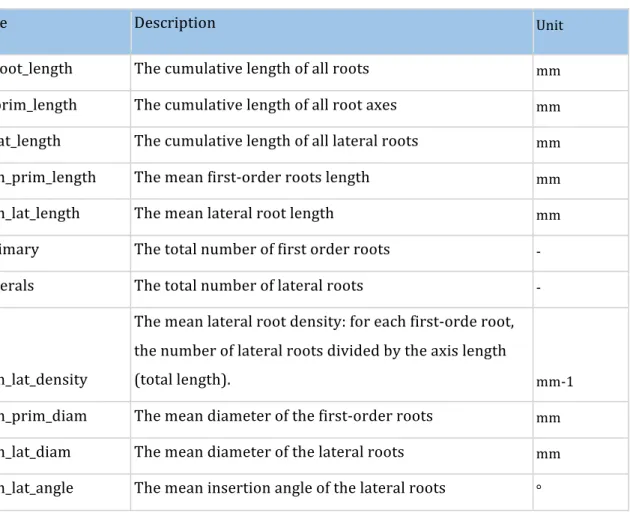
growth was enabled (the extend of which was determined by a random parameter) . For all 110 simulation, only first order laterals were created, to limit complexity. 111 112 The root system created from each simulation was stored in an RSML file. Each RSML file was then 113 read by the RSML Reader plugin from ImageJ to extract metrics and generate ground-truth data for 114 the library (Lobet et al., 2015). These ground-truth data included geometrical,morphological and 115 topological parameters (table 1). For each RSML data file, the RSML Reader plugin also created a 116 PNG image (at a resolution of 300 DPI) of the root system. 117 118 Table 1: Root system parameters used as ground-truth data 119

Name Description Unit

tot_root_length The cumulative length of all roots mm tot_prim_length The cumulative length of all root axes mm tot_lat_length The cumulative length of all lateral roots mm mean_prim_length The mean first-order roots length mm mean_lat_length The mean lateral root length mm n_primary The total number of first order roots - n_laterals The total number of lateral roots - mean_lat_density The mean lateral root density: for each first-orde root, the number of lateral roots divided by the axis length (total length). mm-1 mean_prim_diam The mean diameter of the first-order roots mm mean_lat_diam The mean diameter of the lateral roots mm mean_lat_angle The mean insertion angle of the lateral roots °

Root image analysis

121 Each generated image was analysed using a custom-made ImageJ plugin, Root Image Analysis-J (or 122 RIA-J). The source code of RIA-J, as well as a compiled version is available at the address: 123 https://zenodo.org/record/61509. 124 125 For each image, we extracted a set of classical root image descriptors, such as the total root length, 126 the projected area or the number of visible root tips. In addition, we included shape descriptors, 127 such as pseudo-landmarks, or a-dimensional metrics such as the exploration ratio, of the width 128 proportion at 50% depth (see Supplemental file 1 for details about the shape descriptors). The list 129 of metrics and algorithms used by our pipeline is listed in the table 2. 130

Data analysis

131 Data analysis was performed in R (R Core Team). Morphometric analyses were performed using the 132 momocs (Bonhomme et al., 2014) and shapes (Dryden, 2015)packages. Plots were created using 133 ggplot2 (Wickham, 2009) and lattice (Sarkar, 2008). 134 The Relative Root Square Mean Errors (RRSME) were estimated using the equation: 135 𝑅𝑅𝑀𝑆𝐸 = (𝑦𝚤 − 𝑦𝑖) 𝑦𝚤 ! 𝑛 where 𝑛 is the number of observations, 𝑦𝚤 is the mean and 𝑦𝑖 is the estimated mean. 136 The Linear Discriminant Analysis (LDA) was performed using the lda function from the MASS 137 package (M and D, 2002). For each analysis, we used the synthetype information as grouping factor. 138 We used half of the samples (5) of each synthetype to build the model and the other half to assess 139 the discriminant power of the each class of metrics (morphology and shape). 140

Data availability

141 All data used in this paper (including the image and RSML libraries) are available at the address 142 https://zenodo.org/record/61739 143 An archived version of the codes used in this paper is available at the address 144 https://zenodo.org/record/152083 145 146

Results and discussions

147

Production of a large library of ground-truthed root system images

148 We combined existing tools into a single pipeline to produce a large library of ground-truthed root 149 system images. The pipeline combines a root model (ArchiSimple (Pagès et al., 2013)), the Root 150 System Markup Language (RSML) and the RSML Reader plugin from ImageJ (Lobet et al., 2015). In 151 short, ArchiSimple was used to create a large number of root systems, based on random input 152 parameter sets. Each output was stored as an RSML file (fig. 2A), which was then used by the RSML 153 Reader plugin to create a graphical representation of the root system (as a .jpeg file) and a ground-154 truth dataset (fig. 2B). Details about the different steps are presented in the Materials and Methods 155 section. 156 157 158

We used the pipeline to create a library of 10,000 root system images, separated into monocots 159 (multiple first order roots and no secondary growth) and dicots (one first order root and secondary 160 growth). For each input parameter-set used for ArchiSimple (1.000 different ones), 10 repetitions 161 were performed to create synthetic genotypes, or synthetypes (fig. 2A). The synthetype repetitions 162 were done such as the structure of the final dataset would mimic the structure of a dataset 163 containing phenotypic data of different genotypes. The ranges of the different ground-truth data are 164 shown in table 2 and their distribution is shown in the Supplemental Figure 1. The pipeline 165 produced perfectly thresholded black and white images and hence the following analyses were 166 focused on the characterisation of the root objects themselves. 167 168 We started by evaluating whether monocots and dicots should be separated during the analysis. We 169 performed a Principal Component Analysis on the ground-truthed dataset to assess if the species 170 grouping had an effect on the overall dataset structure (fig. 3A). Monocots and dicots formed 171 distinct groups (MANOVA p-value < 0.001), with only minimal overlap. The first principal 172 component, that represented 33.2% of the variation within the dataset, was mostly influenced by 173 the number of primary axes. The second principal component (19.6% of the variation) was 174 influenced, in part, by the root diameters. These two effects were consistent with the clear grouping 175 of monocots and dicots, since they expressed the main difference between the two species. 176 Therefore, since the species grouping had such a strong effect on the overall structure, we decided 177 to analyse them separately rather than together for the following analyses. 178 179

Table 3: Ranges of the different ground-truth data from the root systems generated using

180

ArchiSimple 181

variable minimum value maximum value unit

MONOCOTS tot_root_length 8.36 2455.03 cm width 0.25 33.21 cm depth 5.49 37.5 cm n_primary 1 20 - tot_prim_length 6 327 cm mean_prim_length 3.22 38 cm mean_prim_diameter 0.02 0.04 cm mean_lat_density 0 100.88 cm n_laterals 0 1378 - tot_lat_length 0 1630 cm mean_lat_length 0 4.44 cm mean_lat_diameter 0 0.03 cm mean_lat_angle 0 97.74 ° DICOTS tot_root_length 6.91 585.05 cm width 0.01 15.05 cm depth 3.89 36.99 cm n_primary 1 1 - tot_prim_length 4 37 cm mean_prim_length 4.4 37.5 cm mean_prim_diameter 0.02 1.13 cm mean_lat_density 0 494.54 cm n_laterals 0 277 - tot_lat_length 0 437 cm mean_lat_length 0 5.48 cm mean_lat_diameter 0 0.23 cm mean_lat_angle 0 87.63 ° 182

Systematic evaluation of root image descriptors

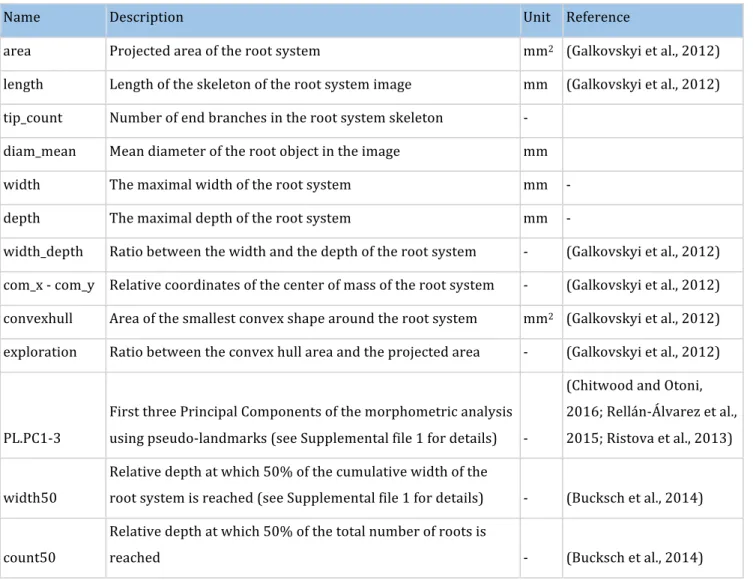
184 In order to demonstrate the utility of a synthetic library of ground-truthed root systems, we 185 analysed every image of the library using a custom-built root image analysis tool, RIA-J. We decided 186 to do so because our purpose was to test the usefulness of the synthetic analysis and not to assess 187 the accuracy of existing tools. Nonetheless, RIA-J was designed using known and published 188 algorithms, often used in root system quantification. A detailed description of RIA-J can be found in 189 the Materials and Methods section. 190 191

Table 3: Root image descriptors extracted by RIA-J

192

Name Description Unit Reference

area Projected area of the root system mm2 _{(Galkovskyi et al., 2012)}

length Length of the skeleton of the root system image mm (Galkovskyi et al., 2012) tip_count Number of end branches in the root system skeleton -

diam_mean Mean diameter of the root object in the image mm

width The maximal width of the root system mm -

depth The maximal depth of the root system mm -

width_depth Ratio between the width and the depth of the root system - (Galkovskyi et al., 2012) com_x - com_y Relative coordinates of the center of mass of the root system - (Galkovskyi et al., 2012) convexhull Area of the smallest convex shape around the root system mm2 _{(Galkovskyi et al., 2012)}

exploration Ratio between the convex hull area and the projected area - (Galkovskyi et al., 2012)

PL.PC1-3 First three Principal Components of the morphometric analysis using pseudo-landmarks (see Supplemental file 1 for details) - (Chitwood and Otoni, 2016; Rellán-Álvarez et al., 2015; Ristova et al., 2013) width50 Relative depth at which 50% of the cumulative width of the root system is reached (see Supplemental file 1 for details) - (Bucksch et al., 2014) count50 Relative depth at which 50% of the total number of roots is reached - (Bucksch et al., 2014)

We extracted 16 descriptors from each root system image (Table 3) and compared them with their 194 own ground-truth data. For each pair of descriptor/data, we performed a linear regression and 195 computed its r-squared value. Figure 4 shows the results from the different combinations for both 196 monocots and dicots. We can observe that, as a general rule, good correlations were rare, with only 197 3% of the combinations having an r-squared above 0.8. In addition, even a good correlation is not 198 necessarily directly useful as the relationship between the two variables might not follow a 1:1 rule 199 (fig. 4B-C). In such case, an additional validation might be needed to define the relation between 200 both variables. 201 202 It also has to be noted that the correlations were different between species. As an example, within 203 the dicot dataset, no good correlation was found between the tip_count and diam_mean estimators 204 while better correlation was found for the monocots. As a consequence, validation of the different 205 image analysis algorithms should be performed, at least, for each group of species. An algorithm 206 giving good results for a monocot might fail when applied on dicot root system analysis. 207

Errors from image descriptors are likely to be non linear

209 In addition to being related to the species of study, estimation errors are likely to increase with the 210 root system size. As the root system grows and develops, the crossing and overlapping segments 211 increase, making the subsequent image analysis potentially more difficult and prone to error. 212 However, a systematic analysis of such error is seldom performed. 213 214 Figure 5 shows the relationship between the ground-truth and descriptor values for three 215 parameters: the total root length (fig. 5A), the number of roots (fig. 5B) and the root system depth 216 (fig. 5C). For each of these variables, we quantified the Relative Root Mean Square Error (see 217 Materials and Methods for details) as a function of the total root length. We can observe that for the 218 estimation of both the total root length and the number of lateral roots, the Relative Root Square 219 Mean Error increased with the size of the root system (fig. 5A-B). As stated above, such increase of 220 the error was somehow expected with increasing complexity. For other metrics, such as the root 221 system depth, no errors were expected (depth is supposedly an error-less variable) and the Relative 222 Root Mean Square Error was close to 0 whatever the size of the root system. 223 224 Such results are a call to caution when analysing root images as unexpected errors in descriptors 225 estimation can arise. This is probably even more true with real images, that are susceptible to 226 contain non-root objects (e.g. dirt) and lower order laterals roots (as stated above, simulations used 227 here were limited to first order laterals). 228

229

230 231

Differentiation power differs between metrics

232 Finally, we wanted to evaluate which metrics were the most useful to discriminate between root 233 systems of different genotypes or experimental series (control vs treatment). As explained above, 234 for each parameter set used in the ArchiSimple run for library construction, we generated 10 root 235 systems. Given the intrinsic variability existing in the model, each of these 10 root systems were 236 similar although different, as could be expected from plants of the same genotype. These so-called 237 synthetypes, were then used to evaluate how efficient were the different metrics to discriminate 238 them. 239 240 To estimate the differentiation of the image metrics, we used a Linear Discriminant Analysis (LDA) 241 prediction model. For each synthetype, half of the plants were used to create the LDA model. The 242 model was then used to predict a synthetype for the remaining half of the plants. This approach 243 allowed us to evaluate the prediction accuracy, or differentiation power, of the different metrics. A 244 prediction accuracy of 100% means that all plants were correctly assigned to their synthetype. To 245 evaluate the differentiation power of single metrics, we used an approach in which each metric was 246 iteratively added to the model, based on the model global prediction power (see Supplemental 247 Figure 3 for details about the procedure) . We performed the analysis either on a full dataset (fig. 248 6D-E), or on a data restrictedto the smallest plants (fig. 6A), in order to test the influence of the 249 underlying data structure. 250 251 Two main observations can be made on the figure 6. First, for three out of four scenarios, only 5 (or 252 less) descriptors were needed to achieve a differentiation accuracy of 90%. Depth, area and length 253

handful of variables were sufficient to distinguish synthetypes, and by extension genotypes or 256 treated plants. However, we can also observe that the most important parameters changed 257 depending on the underlying data structure (either due to species or the size of the dataset). This 258 indicates that it is difficult to have an a priori evaluation of the important variables. Keeping as 259 many variable a possible might always be the most efficient solution. 260 261

Conclusions

263 The automated analysis of root system images is routinely performed in many research projects. 264 Here we used a library of 10.000 modelled images to estimate the accuracy and usefulness of 265 different image descriptors extracted with an home-made root image analysis pipeline. The analysis 266 highlighted some important limitations during the image analysis process. 267 268 Firstly, general structure of the root system (e.g monocot vs dicots) can have a strong influence on 269 the descriptors accuracy. Descriptors that have been shown to be good predictors for one type of 270 root systems might fail for another type. In some cases, the calibration and the combination of 271 different descriptors might improve the accuracy of the predictions, but this needs to be assessed 272 for each analysis. 273 274 A second factor influencing strongly the accuracy of the analysis is the root system size and 275 complexity. As a general rule, for morphological descriptors, the larger the root system, the larger 276 the error is. So far, a large proportion of the root research has been focused on seedlings with small 277 root systems and have de facto avoided such errors. However, as the research questions are likely 278 to focus more on mature root system in the future, these limitations will become critical. 279 280 Finally we have shown that not all metrics have the same benefit when comparing genotype or 281 treatments. Again, depending on the root system type or size, different metrics will have different 282 differentiation powers. 283 284 It is important to highlight that the images used in our analysis were perfectly thresholded, without 285 any degradation in the image quality. Therefore, the errors computed in our analysis are likely 286

under-estimated compared to real images (with additional background noise and lesser quality). 287 Since the quality of the images is dependent on the underlying experimental setup, artificial noise 288 could be added to the generated images in order to mimic any experimentally induced artifact and 289 to improve the analysis pipeline evaluation, as proposed by (Benoit et al., 2014). 290 291 To conclude, our study is a reminder that thorough calibrations are needed for root image analysis 292 pipelines. Here we have used a large library of simulated root images, that we hope will be helpful 293 for the root research community to evaluate current and future image analysis pipelines. 294 295 296

Conflict of Interest

297 The authors declare that the research was conducted in the absence of any commercial or financial 298 relationships that could be construed as a potential conflict of interest. 299

Author Contributions

300 GL, LP, PT and CP designed the study. IK developed the image analysis pipeline RIA-J. GL generated 301 the image library, did the image analysis and data analysis. LP developed the ArchiSimple model. All 302 authors have participated in the writing of the manuscript. 303

Funding

304 This research was funded by the Interuniversity Attraction Poles Programme initiated by the 305 Belgian Science Policy Office, P7/29. GL is grateful to the F.R.S.-FNRS for a postdoctoral research 306 grant (1.B.237.15F). 307

Supplementary Material

308 - Supplemental figure 1: Distribution of the properties of the modelled root images 309 - Supplemental figure 2: Distribution of the descriptors of the modelled root images 310 - Supplemental figure 3: Workflow used for the accuracy analysis 311 - Supplemental file 1: Defintions of the shape descriptors 312 313

References

314 Armengaud, P., Zambaux, P., Hills, A., Sulpice, R., Pattison, R. J., Blatt, M. R., et al. (2009). EZ-Rhizo: integrated 315 software for the fast and accurate measurement of root system architecture. Plant J 57, 945–956. 316 Benoit, L., Rousseau, D., Belin, É., Demilly, D., and Chapeau-Blondeau, F. (2014). Simulation of image 317 acquisition in machine vision dedicated to seedling elongation to validate image processing root 318 segmentation algorithms. Computers and Electronics in Agriculture 104, 84–92. 319 doi:10.1016/j.compag.2014.04.001. 320 Bonhomme, V., Picq, S., and Gaucherel, C. (2014). Momocs: outline analysis using R. Journal of Statistical …. 321 Bucksch, A., Burridge, J., York, L. M., Das, A., Nord, E., Weitz, J. S., et al. (2014). Image-based high-throughput 322 field phenotyping of crop roots. doi:10.1104/pp.114.243519. 323 Chitwood, D. H., and Otoni, W. C. (2016). Morphometric analysis of Passiflora leaves I: the relationship 324 between landmarks of the vasculature and elliptical Fourier descriptors of the blade. 325 doi:10.1101/067512. 326 Dryden, I. L. (2015). shapes package. Vienna, Austria. 327 Galkovskyi, T., Mileyko, Y., Bucksch, A., Moore, B., Symonova, O., Price, C. A., et al. (2012). GiA Roots: software 328 for the high throughput analysis of plant root system architecture. BMC Plant Biol 12, 116. 329 doi:10.1186/1471-2229-12-116. 330 Koevoets, I. T., Venema, J. H., Elzenga, J. T. M., and Testerink, C. (2016). Roots Withstanding their 331 Environment: Exploiting Root System Architecture Responses to Abiotic Stress to Improve Crop 332 Tolerance. Front Plant Sci 07, 91–19. doi:10.3389/fpls.2016.01335. 333 Lobet, G., Pound, M. P., Diener, J., Pradal, C., Draye, X., Godin, C., et al. (2015). Root System Markup Language: 334 Toward a Unified Root Architecture Description Language. Plant Physiol 167, 617–627. 335 doi:10.1104/pp.114.253625. 336 M, V. W., and D, R. B. (2002). Modern Applied Statistics with S 337 . New-York: Springer. 338

Pagès, L., Bécel, C., Boukcim, H., Moreau, D., Nguyen, C., and Voisin, A.-S. (2013). Calibration and evaluation of 342 ArchiSimple, a simple model of root system architecture. Ecological Modelling 290, 76–84. 343 doi:10.1016/j.ecolmodel.2013.11.014. 344 Pagès, L., Jordan, M. O., and Picard, D. (1989). A simulation model of the three-dimensional architecture of the 345 maize root system. Plant and Soil 119, 147–154. doi:10.1007/BF02370279. 346 Pagès, L., Vercambre, G., Drouet, J.-L., Lecompte, F., Collet, C., and LeBot, J. (2004). RootTyp: a generic model 347 to depict and analyse the root system architecture. Plant and Soil 258, 103–119. 348 Pierret, A., Gonkhamdee, S., Jourdan, C., and Maeght, J.-L. (2013). IJ-Rhizo: an open-source software to 349 measure scanned images of root samples. Plant and Soil, 1–9. doi:10.1007/s11104-013-1795-9. 350 R Core Team R: A Language and Environment for Statistical Computing. 351 Rellán-Álvarez, R., Lobet, G., Lindner, H., Pradier, P.-L., Sebastian, J., Yee, M.-C., et al. (2015). GLO-Roots: an 352 imaging platform enabling multidimensional characterization of soil-grown root systems. eLife 4, 353 e07597. doi:10.7554/eLife.07597. 354 Ristova, D., Rosas, U., Krouk, G., Ruffel, S., Birnbaum, K. D., and Coruzzi, G. M. (2013). RootScape: A landmark-355 based system for rapid screening of root architecture in Arabidopsis thaliana. 356 doi:10.1104/pp.112.210872. 357 Sarkar, D. (2008). Lattice: Multivariate Data Visualization with R. New York: Springer. 358 Wickham, H. (2009). ggplot2. New York, NY: Springer New York doi:10.1007/978-0-387-98141-3. 359 360