O
pen
A
rchive
T
OULOUSE
A
rchive
O
uverte (
OATAO
)
OATAO is an open access repository that collects the work of Toulouse researchers and
makes it freely available over the web where possible.
This is an author-deposited version published in :
http://oatao.univ-toulouse.fr/
Eprints ID : 14741
To cite this version :
Fontoura Cupertino, Leandro and Da Costa, Georges and Sayah,
Amal and Pierson, Jean-Marc Valgreen: an Application's Energy Profiler. ( In Press:
2013) International Journal of Soft Computing and Software Engineering, vol. 3 (n° 3).
pp. 549-556. ISSN 2251-7545
Any correspondance concerning this service should be sent to the repository
administrator: [email protected]
Valgreen: an Application’s Energy Profiler
Leandro Fontoura Cupertino, Georges Da Costa, Amal Sayah, Jean-Marc Pierson
University of Toulouse, France
Email: {fontoura, dacosta, sayah, pierson}@irit.fr
Abstract. The popularity of hand-held and portable devices put the energy aware computing in
evidence. The need for long time batteries surpasses the hardware manufacturer, impacting the operational system policies and software development. Power modeling of applications has been studied during the last years and can be used to estimate their total energy. In order to aid the programmer to implement energy efficient algorithms, this paper introduces an application’s energy profiler, namely Valgreen, which exploits the battery’s information in order to generate an architecture independent power model through a calibration process.Keywords
: application, energy, profiler, power, model* Corresponding Author: Leandro Fontoura Cupertino,
Toulouse Institute of Computer Science Research (IRIT), University of Toulouse III (Paul Sabatier), Toulouse, France, Email: [email protected] Tel:+33 (0)5 61 55 64 18
1. Introduction
Application profilers are well known tools for deploying codes during software’s development to improve their performance. They help programmers to identify application’s bottlenecks by reporting some of its characteristics that can only be gathered during its execution. Profilers differ from each other concerning their sampling methodology and their collected metrics. The main metrics evaluated are: execution time [1], memory allocation [2] and network load [3]. Regarding the methodology, there are three main approaches: event-based, instrumenting and statistical profiling. The event-based method can only be used for interpreted languages and provides profiler’s access as an event occurs. Instrumenting consists of inserting code during the compilation phase of the application to allow profiler's access. The statistical approach samples a metric at regular time-steps. The latest method is the less invasive one and can be used to collect information from any application, even if no source code is available.
Portable devices, such as notebooks, tablets and smartphones, brought the problem of battery lifetime duration to the mainstream. A lot of work to enhance battery’s duration has been done on the hardware level, such as dynamic voltage and frequency scaling and devices idle states policies [4, 5, 6]. Although the hardware capabilities are the main actors of the power savings, the usage of such hardware is led by the software that it executes, i.e., the power consumption of hardware varies according to the software it is running.
Some application’s power monitoring tools have already been proposed, however there is still a lack of a profiling tool to aid developers to write energy efficient codes by reporting the total energy spent to execute them. In addition, this information can feed the operating system so that it can manage whether an application will be executed based on the remaining energy that the battery can provide. Furthermore, a similar approach can be used on distributed and cloud systems to decide where an application will run on a datacenter.
This paper introduces Valgreen, a new statistical profiling tool which details the energy consumed by an application. Valgreen uses a home-made open source library of sensors, namely Energy Consumption library (libec) [13] to explore several application sensors in order to estimate the energy required by the application to be completely executed.
The remaining of this paper is divided as follows. Section 2 reviews the related works. Section 3 presents the used techniques to estimate the power of an application. Section 4 describes how the profiling tool was conceived. In section 5 the compiler’s optimization options are evaluated. Finally, some conclusions are drawn in section 6.
2. Related Work
Back in 1982, Graham et all proposed an instrumental execution profiler that attributes the execution time of subroutines into the time of the routine that called them [1]. From this moment on,
gprof became one of the most popular profilers used to locate application’s hotspots, enabling the
programmer to focus on the optimization of the most critical methods. Another well-known profiler was presented in [2]. Valgrind is a dynamic binary instrumentation framework mostly used to detect memory leaks. Both, Valgrind and gprof are helpful tools to enhance the performance of applications, but they give no information about the energy used to execute such codes.
PowerScope [7] was the first tool able to profile the energy usage by applications. It requires an
external monitoring infrastructure composed by three elements: a digital multi meter to measure the power dissipated by a node; a data collection computer to monitor its energy; and a profiling computer to monitor system’s variables while executing the application and to compute its energy profile afterwards. The collected information from the physical machine’s power is transmitted to the application level according to which process was running when the power was collected. This approach is limited for single core architectures, in which only one application can be executed at a time. Furthermore, it can mix the consumption of different processes on peripheral devices such as disks or network. Additionally, it does not consider the systems idle power separately.
In 2007, Intel released a tool to monitor the power leakage on a computer, namely PowerTOP [8]. It estimates the most power consuming programs or drivers based on their wakeups per second rate, which prevent the CPU to enter on the idle modes (C-states). Based on this information, it suggests some system configurations to improve power savings. Other power monitoring tools, such as pTop [9] and pTopW [10], have a similar approach, proposing different models for estimation of the application’s power. Even though, none of these tools can provide application’s energy directly.
Recently, PowerAPI [11] enables the profiling of application’s energy by an estimation that is totally independent of external hardware, such as power meters. To estimate the power consumed by a computer, it aggregates the estimated power consumed by its components such as CPU, network and disk. Hence, it depends on the power modeling of such devices. PowerAPI subsystems’ power models require as inputs some hardware’s specifications which may or may not be provided by their vendors. Its models do not take into account idle and chassis power consumption, therefore, the accumulated power of all applications does not match the measurements from an external power meter. Moreover, the proposed API was developed for servers and do not models features as simultaneous multithreading.
Our approach differs from these tools by providing an energy profiling of applications with an architecture independent model that can be calibrated whether a watt meter is available. We create a parameterless power model which exploits a common feature on portable devices: an embedded power meter. Portable devices depend on batteries that can provide instant voltage and current consumption while discharging at no additional costs.
3. Power of Applications
The main issue when modeling the power of application is to validate it since it is impossible to directly measure its power with a watt meter. Therefore, one needs to make some assumptions to correlate the power drained by the machine with the one dissipated by the applications that it executes. In our case, we assume that the power of each application running on a machine is independent and that they can be aggregated in order to sum the total power consumption of the entire machine as follows:
å
"
Î
pid pid mac=
P
,
pid
RP
P
(1)where
P
mac andP
pid are, respectively, the machine and process power, andRP
is the set of all processes currently running on the machine. Based on this conjecture one can validate its model byusing a power meter and comparing the measured power with the sum of all the processes’ estimation. Some authors prefer to consider the idle power to be independent of the process, we believe that if the machine is turned on, it must be running at least one process, even if it is a kernel process and this process needs to account the idle power, otherwise this machine could be shut down.
The most used approach for modeling the power dissipated by applications is to identify all the hardware devices on the system and create a relation between them and the process:
å
"
Î
dev dev pid pid=
P
,
dev
D
P
(2)where
D
is the set of all devices present at the machine. The power modeling of devices can be as complex and accurate as one may need. Typically, these models takes into account only the most power consuming devices and need information that are specific for each device.In order to create an architecture independent model, we propose a calibration process based on machine learning algorithms to avoid device’s specific data dependency. The details of such approach are described in the next session.
4. Valgreen
Valgreen is a statistical profiler which samples the power of an application in short time steps and
measures the total energy spent during the execution of such application. It has a power model which can be used statically or may exploit the advantage of having a power meter to calibrate itself.
On
portable devices, the power dissipated by the battery can be collected through the Advanced Configuration and Power Interface (ACPI) at no additional cost, while on datacenters this information can be retrieved from external watt meters that need to be installed. The ACPI information can only be used to measure the dissipated power when the battery is discharging. In other words, this information can be interrupted at any time. Valgreen takes this issue into account, being immune to it. When used at static mode, its power estimator do not depend on the actual watt meter data, while during the calibration process, the data will only be collected if the current power is available.
It is known that the devices that impacts most on the total power dissipated by a machine are the CPU, memory and hard disk [12], although for portables devices, the wireless network interface card and screen can also have a great impact. Since the most consuming device is the CPU, the default mathematical model used to estimate the power of applications in Valgreen is a CPU proportional model, described as:
| |
å
"
Î
cpu 2 idl cpu cpu pid 1 0 pid,
cpu
C
RP
w
+
t
+
t
t
w
+
w
=
P
1
(3)where
t
cpu ,t
idl andt
cpupid are, respectively, the total, idle and process’ CPU time,C
is the set of all processors available,| |
RP
is the cardinality of the running processes set and the weight vector[
w
,
w
1,
w
2]
=
w
0 is the set of architecture dependent parameters. The power estimator used in this profiler can be easily changed to match the machine needs by adding or removing device specific sensors. Besides, other models can be used, one can even define if the profiler will use the power meter information in a reverse model, commuting to a power model when the watt meter is not available (for portable devices this happens when it is plugged on the outlet).The estimation of application’s power depends on the application behavior. This behavior can be measured by sensors that collect data related to the hardware usage, such as CPU time, memory and networking usage. To measure the power dissipated by an application in a given moment, Valgreen exploits some operating system sensors available on the Energy Consumption library, namely libec [13]. libec is an open source modular library with a set of sensors related to energy consumption. A sensor is defined as a direct metric or an estimated value. A direct metric is a physical measurement, while an estimator aggregates a value to the direct metric in order to measure a new property. Currently, the sensors implemented in this library are mainly based on hardware performance counters and operational system information, but libec sensors can easily be extended to collect different data coming from any source. Its sensors can be divided into two classes: machine and application related sensors.
Machine related sensors can only measure a property for the entire computing system, e.g., power meter can only provide information related to the power measured on the outlet, which concerns all devices and processes running on a machine. Among the available machine level sensors, Valgreen uses the running processes and ACPI power meter. The former gives the total number of processes which were executed during the last time step, while the latter collects information from the actual current and voltage from the battery to estimate its dissipated power.
Application related sensors can retrieve information for a specific process. Valgreen uses the CPU time usage sensor, which calculates the CPU usage percentage for a given process based on its CPU system and user elapsed times.
Valgreen’s power model can be calibrated to fit better the characteristics of the host machine. As
stated before, to validate a power model for the application level, one needs to correlate them somehow with the machine as a whole. For the calibration process this is done aggregating all running processes’ power as follows:
| |
å
å
"
Î
Î
cpu 2 idl cpu cpu 1 0 pid pidmac
+
w
,
cpu
C,
pid
RP
t
+
t
t
w
+
RP
w
=
P
=
P
(4)The calibration phase of the algorithm is done through linear regression, using the mean squared error as the metric of error. In order to apply such algorithm we first need to collect historical data with information from the sensors and the power dissipated in a given time. Each line on the matrix
X
and the vectory
is one history data for the sensors and ACPI power meter, respectively. Then, the calibrated weights will be given by:y
X
=
w
-1 , (5) whereX
-1 is the pseudo inverse ofX
,y
is the target vector andw
is the vector of parameters to be calibrated. The quality of the historical data during the calibration is of great importance. In order to collect significant data, the calibration phase must guarantee that the data is valid and that it ranges the whole spectrum of variables.According to the hardware characteristics the response time of the ACPI power meter can be from the order of milliseconds to tens of seconds. When sampling data from a watt meter with high latency such as ACPI, one needs to be careful with its sampling frequency. Valgreen takes this issue into account during the calibration process of its model by detecting the ACPI’s refresh rate in order to properly configure the frequency to collect the data values to be used by the calibration process.
Nevertheless, the calibrated model will only fit well for the historical data characteristics, this means that if all the data were collected while the system was idle, it will only be able to estimate the idle power. To vary the device's load and collect good-enough data to be fit, Valgreen uses the Linux stress command, a tool which contains micro benchmarks developed to stress the CPU, memory, disk and network during a given amount of time.
Once the model is well calibrated, the proposed profiler needs to calculate the total energy spent during the execution of an application. Valgreen computes this energy by sampling the application's power in very short time periods. When measuring the energy spent for an application, the most fine-grained it is done, the better, because the short time difference between two updates will decrease the chance of missing power fluctuations that may occur during small time steps. The duration of such time step can be set by the user.
5. Experimental Results
The experiments on this paper are divided into three parts. First, in subsection 5.1, we define our hardware setup. We first analyze the ACPI’s accuracy in subsection 5.2. In subsection 5.3, we validate our calibration methodology by comparing it with some user defined parameterization. Subsection 5.4 evaluates the importance of having a power model for a fine grained analysis, through the comparison of an ACPI power output against our calibrated model. Finally, subsection 5.5 illustrates the results on a real use case, compiling a linear algebra library using all of the GNU’s optimization flags and executing the profiler with distinct workloads to compare their dissipated energy.
5.1. Environment Setup
All experiments were done using a Dell Latitude D830 laptop with an Intel Core 2 Duo T8300 at 2.40GHz processor, 2GB DDR2-667 SDRAM memory, 15.4’’ Wide Screen WUXGA LCD and 120GB ST9120823ASG hard disk. As operational system we used Scientific Linux release 6.3 (Carbon). During all experiments, CPU’s hyper threading was disabled. To collect the ACPI power, the battery was fully charged and then the power line was unplugged from the outlet.
5.2. ACPI as a Power Meter
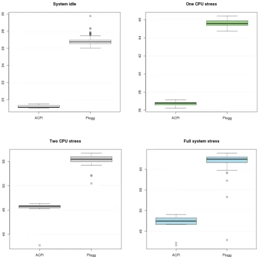
To test the usage of ACPI as a power meter, we compared it with Energy Optimizers Limited’s Plogg, an outlet adapter used to measure the dissipated power of appliances. To collect Plogg’s data, the battery need to be removed from the laptop to avoid unwanted capacitances and battery discharges during the experiments. To compare both watt meters, four distinct workloads were executed on our system, under the same conditions, i.e., all of them ran in run-level 3 just after the machine is booted. The first workload is the idle system, in which we just execute a sleep command during 4 minutes. The second and third ones are CPU stress workloads for one and two CPU’s, respectively, given by the execution of the Linux stress command with a timeout of 3 minutes each. Finally, we used the same command to stress the full system including memory and disk, with a timeout of 3 minutes as well.
Figure 1. Comparison between ACPI and Plogg power meters for distinct workloads Figure 1 presents the box-plots of the collected data. The y-axis reflects the power consumption. As one can see, the power given by the ACPI power meter is lower than the Plogg’s one for all workloads. This was expected due to the type of current we are measuring, with the ACPI we collect data related to the DC drained by the battery, while Plogg gets its data before the AC/DC conversion, which has
losses. The analysis of the difference between the mean values of each workload shows that the AC/DC conversion losses grow along with the dissipated power, which was also an expected result. These losses pass from 7 watts on idle mode to 15 watts on full system stress, which means that around 25% of the energy is lost during this conversion. One can see that ACPI data has less variance than the Plogg for all workloads, which means that it is more stable and possibly more accurate.
5.3. Calibration Phase
The first step to be done is to discover the update frequency of the ACPI power meter. To do so, we wait for the first variation of power given by the ACPI sensor, and then we reset the stopwatch and keep monitoring the power of ACPI in 100 ms intervals, when the given power changes again we keep the data from the stop watch as the ACPI latency in milliseconds. This works well because even during an idle state, the ACPI power varies. With this information, one can estimate the total duration of the benchmark execution in order to have sufficient data to learn all the parameters. Finally, we collect the data regarding our model’s inputs (CPU time and running processes) and output (dissipated power) while running several micro benchmarks available on the Linux stress package, which can stress the CPU, memory, network and hard disk.
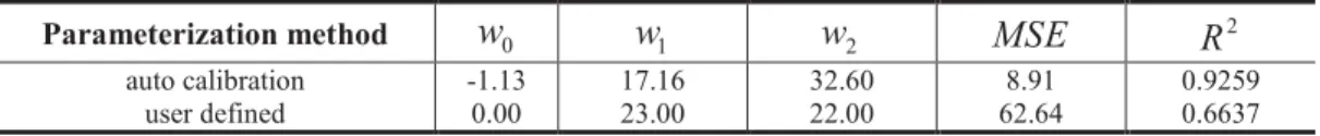
To evaluate the calibration process we compared the calibrated parameters with a user defined parameterization. The user’s parameterization is given as follows:
w
0=
0
,w
1=
(P
max-
P
idl)
andidl
P
=
w
2 , whereP
max is the maximum total power consumed by the node during the benchmark execution. Although this is a quite intuitive parameterization for such model, it uses some device specific data, than can be collected during the execution of benchmarks or even during the production phase of the machine.Table 1 compares the two parameterization approaches. On the first three columns we have the parameters for our model, while the two last has some accuracy metrics. As one can see the major difference between these models are on the third parameter, which is related to the total number of active processes running on the node. This parameter defines the portion of the idle power that is attributed to a process. On the error metrics columns we have the mean squared error (
MSE
) and the correlation coefficient(
R )
2 . The MSE is used as the learning error metric, while theR
2 gives an idea of the percentage of the variation of the target output can be explained by the model, varying from zero (no correlation at all) to one (maximum).Table 1. Comparison between automatic calibration and predefined parameters for the power model
Parameterization method
w
0w
1w
2MSE
R
2auto calibration user defined -1.13 0.00 17.16 23.00 32.60 22.00 8.91 62.64 0.9259 0.6637 The results show that the model can be quite accurate when properly calibrated. The
MSE
of the calibrated is around 7 times better than the user defined one. Moreover, the calibrated parameters the correlation reached 92%, which corresponds to a really good result given such a simple power model.5.4. ACPI Update Frequency Analysis
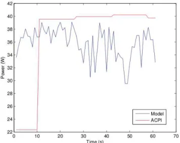
The availability of the battery power consumption implies a cost that not every vendor agrees to pay. This cost is mainly represented by the frequency at which the mother board’s micro controller can update its drained current and voltage. For an accurate measure of the power on a machine, one needs to take into account its update frequency. To illustrate the importance of a high frequency update, we collected the data from the entire machine, applied the calibrated linear model of equation 4 and the power provided by our ACPI sensor.
The results of this experiment are summarized in Figure 2. One can see that the application starts at time zero and the ACPI power meter will only detect this change of behavior 10 seconds later, while the linear model updates its value at each time step (one second in our case). For the following data this refresh time increases to 16 seconds. This poor update frequency makes the ACPI a bad tool for seeing peaks and changes of power consumption in applications even if a good inverse model is being used. The total energy measured from the ACPI data can be far from the real one for applications that
changes their behavior for small time duration. For instance, an application that executes on time intervals which are multiple of the ACPI latency, such as some monitoring applications, will have no impact at all on the ACPI power meter.
Figure 2. Comparison between ACPI power meter and the linear model
5.5. Compilation Flags and Workloads Use Case
The last experiment consists of a real use case. It compares the impact of the compilation options and its workload on the total energy consumed by the application. For this use case we used a well-known linear algebra library, namely LAPACK [14]. The library was compiled using all GNU’s compiler optimization options (-O0, -O1, -O2 and -O3). The resulting codes were used to execute several instances of the LU decomposition problem, which is one of the most used methods to solve linear system of equations. The LU instances vary according to the size of the squared matrix A we want to decompose. During these experiments, the matrix A size varied from 2000x2000 to 5000x5000, which is the maximum matrix size which fits into memory during the entire decomposition, avoiding page faults and consequential changes in power consumption.
Figure 3 shows the total energy consumed by the LAPACK library to compute the squared matrix decomposition for each optimization flag used. The width of the squared matrix A is presented on the horizontal axis. One can see that when dealing with small size problems the optimization parameter do not influences too much, but at the problem size grows, some differences starts to appear. It is interesting to observe that the -O0 parameter, that has no optimization appears as a good energetic solution at first. But for the biggest problems it is the poorest. In the other hand, the -O1 parameter have a mean energy with less variance and can be used for a broader utilization of the solver.
The results presented on figure 3, shows that even a simple decision as the optimization flag can have a great impact on the overall energy consumption of the application. Valgreen can be used not only to detect which optimization option should be used but also to decide between two libraries or implementation patterns, for instance.
6. Conclusions
The popularity of portable devices brought the attention for the importance monitoring the application dissipated power as well as of profiling the total energy spent by an application. The knowledge of how much energy an application will need to be executed can be used from the software engineering perspective, up to the datacenter’s resource scheduling policies.
In this paper, we introduced Valgreen, an application energy profiler distributed under GPL's license that exploits portable device’s batteries to generate more accurate power models. Our results show that the calibration of a model is necessary, and can increase the accuracy of the model up to 7 times. Moreover, a well-defined model can be more accurate than ACPI power meter due to its high frequency of update, our model can go up 10Hz while the ACPI present on our machine operates at 0.0625Hz. Finally, we showed how the total energy dissipation of an application can help programmers choose a more energy efficient library during the development of new software.
As future work we propose to make the a comparison between similar libraries like MKL/Atlas to evaluate which one is more energy efficient for a given usage. Besides, we want to make our profiler more fine grained, going from the process to the function level. Furthermore, the power consumption of distributed applications made of parallel tasks can also be measured and will be studied in order to evaluate the power of such application on a datacenter environment. For the time, Valgreen only runs on Linux platforms, we want to make it available to android and windows operating systems as well.
Acknowledgment
The results presented in this paper are funded by the European Commission under contract 288701 through the project CoolEmAll.
References
[1] Graham, S. L., Kessler, P. B., Mckusick, M. K. “gprof: a Call Graph Execution Profiler”. ACM SIGPLAN Notices, vol. 17, no. 6, pp.120–126, 1982. doi:10.1145/872726.806987.
[2] Nethercote, N., Seward, J. “How to Shadow Every Byte of Memory Used by a Program”. In Proceedings of the 3rd international conference on Virtual execution environments (VEE), p.65, 2007. doi:10.1145/1254810.1254820.
[3] Liu, D., Huebner, F. (n.d.). “Application Profiling of IP Traffic”. In Proceedings of the 27th Annual IEEE Conference on Local Computer Networks (LCN), pp.220–229, 2002. doi:10.1109/LCN.2002.1181787.
[4] Pillai, P., Shin, K. G. “Real-Time Dynamic Voltage Scaling for Low-Power Embedded Operating Systems”. ACM SIGOPS Operating Systems Review, vol. 35, no. 5, pp.89, 2001. doi:10.1145/502059.502044.
[5] Choi, K., Soma, R., Pedram, M. “Dynamic Voltage and Frequency Scaling based on Workload Decomposition”. Proceedings of the International Symposium on Low Power Electronics and Design (ISLPED), p.174, 2004. doi:10.1145/1013235.1013282.
[6] Simunic, T., Benini, L., Glynn, P., De Micheli, G. “Dynamic Power Management for Portable Systems”. In Proceedings of the 6th Annual International Conference on Mobile Computing and Networking (MobiCom), pp.11–19, 2000. doi:10.1145/345910.345914.
[7] Flinn, J., Satyanarayanan, M. “PowerScope: A Tool for Profiling the Energy Usage of Mobile Applications”. In Proceedings of Second IEEE Workshop on Mobile Computing Systems and Applications (WMCSA), pp.2–10, 1999. doi:10.1109/MCSA.1999.749272.
[8] van de Ven, A., “PowerTop linux man page”, Intel Corporation, 2007.
[9] Do, T., Rawshdeh, S., Shi, W. “pTop: A Process-level Power Profiling Tool”. In Proceedings of the 2nd Workshop on Power Aware Computing and Systems (HotPower), 2009.
[10] Noureddine, A., Bourdon, A., Rouvoy, R., Seinturier, L. “A Preliminary Study of the Impact of Software Engineering on GreenIT”. In Proceedings of the First International Workshop on Green and Sustainable Software (GREENS), pp.21–27, 2012. doi:10.1109/GREENS.2012.6224251. [11] Chen, H., Li, Y., Shi, W. “Fine-grained power management using process-level profiling”.
Sustainable Computing: Informatics and Systems, vol. 2, no. 1, pp.33–42, 2012. doi:10.1016/j.suscom.2012.01.002.
[12] Chen, H., Wang, S., Shi, W. “Where Does the Power Go in a Computer System: Experimental Analysis and Implications”. In Proceedings of Green Computing Conference and Workshops (IGCC), pp.1–6, 2011. doi:10.1109/IGCC.2011.6008598
[13] Cupertino, L., Da Costa, G., Sayah A., Pierson, J.-M. “Energy Consumption Library”. In Proceedings of Energy Efficiency in Large Scale Distributed Systems (EE-LSDS) Conference, 2013.
[14] Anderson, E., Bai, Z., Bischof, C., Blackford, L. S., Demmel, J., Dongarra, J. J., Du Croz, J., et al. “LAPACK Users’ guide”, 3rd ed., 1999. Retrieved from http://www.netlib.org/lapack/lug/.