AffiliAtions: Rasmussen, LandoLt, BLack, théRiauLt, kuceRa, Gochis, ikeda, and Gutmann—National Center for Atmospheric Research, Boulder, Colorado; BakeR, kochendoRfeR, meyeRs, and haLL—NOAA/Air Resources Laboratory/Atmospheric Turbulence and Diffusion Division, Oak Ridge, Tennessee; fischeR, smith, and nitu—Environment Canada, Toronto, Ontario, Canada
Corresponding Author: Roy Rasmussen, National Center for Atmospheric Research, P.O. Box 3000, Boulder, CO 80307 E-mail: rasmus@ucar.edu
The abstract for this article can be found in this issue, following the table of contents.
DOI:10.1175/BAMS-D-11-00052.1 In final form 19 November 2011 ©2012 American Meteorological Society
NOAA, FAA, and NCAR work together at the NCAR Marshall Field Site to understand the relative accuracies of different instrumentation, gauges, and windshield configurations to
measure snowfall and other solid precipitation.
MotivAtion: AviAtion And CliMAte needs. Precipitation is one of the most impor-tant atmospheric variables for ecosystem research, hydrologic and weather forecasting, and climate monitoring. Despite its importance, accurate mea-surement of precipitation remains challenging. Measurement errors for solid precipitation, which are often ignored for automated systems, frequently
range from 20% to 50% due to undercatch in windy conditions.
Although measurement accuracy can be dif-ficult to obtain and quantify for precipitation, it is extremely important for monitoring and assessing climate variability and change. Reducing measure-ment uncertainties is essential given the projected increases in precipitation over land over the next 100 yr (IPCC 2007). Obtaining climate-quality pre-cipitation data not only requires overlap with existing measurements but also necessitates an ongoing need for intercomparisons and tests of various gauge windshield configurations.
Undercatch of precipitation (Groisman and Legates 1994), resulting from wind-induced updrafts at the gauge orifice and wetting losses on the internal walls of the gauge, significantly affects the quality and accuracy of precipitation data for climate change studies, and is especially relevant for solid precipita-tion (Goodison et al. 1998). Recent collocated snow measurements at the Environment Canada (EC) Centre for Atmospheric Research Experiments (CARE) near Egbert, Ontario, Canada, highlight the large variability in the total snow water equivalent
HOw wELL ARE wE
MEASuRINg SNOw?
The NOAA/FAA/NCAR
Winter Precipitation Test Bed
By Roy Rasmussen, BRuce BakeR, John kochendoRfeR, tiLden meyeRs, scott LandoLt,
aLexandRe P. fischeR, Jenny BLack, JuLie m. théRiauLt, PauL kuceRa, david Gochis,
(SWE) observed over the 2008–09 accumulation pe-riod (Fig. 1). A large number of precipitation gauges and windshield configurations were examined, in-cluding weighing gauges (WG), heated tipping-bucket rain gauges, and a present weather detector (PWD). A GEONOR T-200B in a Double Fence Intercompari-son Reference (DFIR) wind shield (GEONOR DFIR) served as the reference. Of particular note is the extremely poor performance of the heated tipping-bucket gauges as compared with the reference.
While there have been many solid precipitation measurement studies, only a few focused on the accuracy, reliability, and repeatability of automatic precipitation measurements. The most recent com-prehensive study, organized by the World Meteoro-logical Organization (WMO), took place between 1987 and 1993 (Goodison et al. 1998). The national measurement methods (manual observations) for solid precipitation used at the time were assessed. The report highlighted a number of challenges to solid precipitation measurement, including blockage of the gauge orifice by snow capping the gauge or accumu-lating on the side of the orifice walls; wind undercatch of snow due to the formation of updrafts over the gauge orifice; the unknown role of turbulence on gauge catch; and the large variability in gauge catch efficiency for a given gauge and wind speed. Since this
report, an increasing number of automated stations have been providing measurements of precipitation data, including solid precipitation, with strikingly little information on measurement uncertainty.
Recognizing the need for understanding the quality of precipitation data, the Commission for Instruments and Methods of Observation (CIMO) of the WMO established the assessment of methods for measurement and observation of solid precipitation. Initially, a survey was conducted in 2008 to develop a summary of current methods and instruments for measuring solid precipitation. The results of the survey (Nitu and Wong 2010) indicate that many automatic precipitation gauges and windshield con-figurations are currently used for the measurement of solid precipitation. The gauges vary in terms of orifice area, capacity, sensitivity, and configuration. This variety by far exceeds the variety of manual stan-dard precipitation gauges (Goodison et al. 1998). The need for increased precipitation measurement accu-racy requires a review of the current state-of-the-art methodologies in all climate conditions. The WMO CIMO has assumed a leadership role in organizing and conducting an evaluation of gauges for solid pre-cipitation measurements in cold and Alpine climates.
This paper will present recent efforts to under-stand the relative accuracies of different instru-mentation, gauges, and windshield configurations to measure snowfall at the National Center for Atmo-spheric Research (NCAR) Marshall Field Site. The “Background” sec-tion provides a discussion on snow measurement challenges, including the use of the DFIR shield for ground truth. The test site is described in the “Marshall Field Site test bed site description” section. A description of some of the snow gauge and shield testing conducted at the site is pre-sented in the “Snow gauge and wind shield evaluation studies” section, including some discussion of labo-ratory and theoretical modeling of airflow around gauge/shields. The “Snow gauge performance during extreme winter weather condi-tions: 17–19 March blizzard” sec-tion provides a case study of gauge/ shield performance during the 2003 Denver blizzard. The development of a Federal Aviation Administration (FAA)-supported ground deicing
Fig. 1. total precipitation accumulation (melted snow and rain),
2 dec 2008–15 Apr 2009, at the environment Canada CAre site for a variety of gauge and windshield configurations. shield configura-tions include the double Alter (dA), single Alter (sA), no shield (ns), tretyakov (ttk), and the dfir. Wgs include the geonor t-200B (geonor), vaisala vrg 101, fischer and porter (f and p), and pluvio (1 and 2). heated (h) tipping-bucket (tB) gauges include the vaisala, All Weather inc. (AWi), CAe, and tB3. the geonor dfir serves as the reference.
real-time system is described in the “Application of snow gauges to aircraft deicing: LWE system and check time” section. The “New methods to measure snow” section describes two new snow measurement technologies being evaluated. The paper concludes with a summary and discussion.
BACkground. Snow measurements. Measuring precipitation seems relatively straightforward: water falls into a collector and the observer, in either an automated or manual way, measures the depth, volume, or weight. For rainfall, it is almost this easy if we ignore small errors associated with wetting loss and evaporation. Measuring snowfall and snow depth is much more challenging. The environment has a far greater impact on the accuracy of a snow measurement than on a rainfall measurement. For example, the snowfall measurement accuracy is influenced much more by the local wind than rainfall measurement accuracy is. Lighter and slower falling snow hydrometers are more prone to deflection by wind-induced turbulence around the gauge, making snowfall measurements prone to large systematic errors. The measurement environment also presents unique challenges for the observation of snow depth due to redistribution and metamorphosis, which in turn results in high spatial and temporal variability (e.g., Erickson et al. 2005). The measurement of snow depth presents a further challenge if the measurement objective is SWE because snow density is variable. Because of the interplay of numerous processes that affect the height of snow cover on surfaces during snowfall events, the application of complicated algo-rithms using multiple sensors and/or multiple types of sensors is needed to accurately derive snow depth and SWE from changes in the snow cover surface over very short (minute to hour) time scales (Fischer 2011).
Total solid precipitation, liquid equivalent snow-fall rate, SWE, and snow depth are related but are different phenomena. Total solid precipitation is a measurement of the total liquid water accumula-tion of falling snow hydrometeors for a specified period. Liquid water equivalent (LWE) rate is the mass accumulation rate of solid precipitation and is usually expressed in millimeters per hour. SWE is the liquid equivalent of the snow present on the ground, and snow depth is a measurement of the total depth of snow on the ground. Total precipita-tion is convenprecipita-tionally measured with a precipitaprecipita-tion gauge (manual or automated) by weight or by volume. Liquid equivalent snowfall rate is also measured by a precipitation gauge, but over a defined period of time (typical minimum period is 1 min). Snow depth
can be measured manually using a snow board (new snow) and/or a snow ruler or via an automated device. If the snow density is known or estimated, SWE can be converted to snow depth and vice versa.
Total precipitation and liquid equivalent snowfall rate.
Total solid precipitation and liquid equivalent snow-fall rate are conventionally measured using precipita-tion gauges installed above the surface of the ground. Some types of gauges are used to measure all precipi-tation types (liquid and solid) with additional design features required for measuring snow. Volumetric or nonweighing precipitation gauges catch falling snow in a collector. This collector is removed, the snow melted, and poured into a graduated cylinder for measurement. Volumetric snowfall measurements need to be corrected for a wetting loss error, which typically ranges from 0.10 to 0.15 mm per observa-tion but could be as high as 0.3 mm per observaobserva-tion (Goodison et al. 1998). Metcalfe and Goodison (1993) reported that wetting loss for snowfall measurements at some Canadian sites could be as high as 20% of the total winter precipitation. They can also suffer from evaporation or sublimation losses, especially when temperatures during snowfall are relatively high.
Weighing gauges collect falling snow that is melted within the gauge via an antifreeze solution before it is measured by weight differential. Weighing or accumulating gauges are usually automated. A film of oil on the surface of the bucket contents prevents evaporation of the precipitation before the differen-tial bucket weight can be measured. Melting of the snow also prevents the snow from blowing out of the bucket before it can be weighed. A frozen bucket will eventually fill with snow, plug the orifice, and pre-vent further collection and measurement. Weighing gauges are not subjected to a wetting loss error like volumetric gauges. Weighing gauges, like volumetric gauges, can still be prone to snow capping if the ori-fice diameter is not sufficiently large. “Capping and dumping” occurs when the gauge orifice is plugged with accumulating snow that subsequently falls into the gauge bucket. Although manual volumetric gauges also suffer from this, the observer can usu-ally confirm or correct the occurrence. These events are more difficult to confirm or correct with an automated weighing gauge. To eliminate the capping problem, the orifice is usually heated to just above freezing to melt any snow accumulating on the gauge itself (Rasmussen et al. 2001).
The designs of the weighing mechanisms for automated precipitation gauges are numerous and include spring mechanisms and chart recorders,
potentiometers, load cells, optical shaft encoders, and strain sensors. Heated tipping-bucket gauges, cur-rently in use by many WMO member countries, have also been used to measure snowfall rate. These devic-es, however, have not performed as well as weighing precipitation gauges. Metcalfe and Goodison (1993) reported that the standard shielded gauge recorded 150%–200% more precipitation than an unshielded tipping-bucket gauge due to the deformation of the wind field above the unshielded gauge orifice, evapo-ration due to heating of the snow in the funnel, snow removed from the gauge orifice by the wind before it is melted, and clogging of the tipping mechanism. In addition, Larson (1993) has shown that heating tipping buckets catch 28% less precipitation than the standard universal U.S. National Weather Service (NWS) weighing gauge.
There are many challenges for the measurement of solid precipitation regardless of gauge type or mechanism of measurement. The most significant challenge is the measurement of snowfall in a windy environment. Nearly all precipitation gauges expe-rience a reduction in the catch efficiency (CE) of snowfall with increasing wind speed. A precipita-tion gauge installed above the surface of the ground presents a barrier to air flowing around it, causing a deformation of the wind field above the gauge orifice (Sevruk and Klemm 1989). As air flows around and over a precipitation gauge, falling snow hydrome-teors are deflected by the flow and do not enter the gauge. The degree of deflection, which increases with wind speed, is dependent on the profile of the gauge (Sevruk et al. 1991) and the type of wind shield (if any) employed around the gauge (Goodison et al. 1998). Wind bias in the gauge measurement of a snowfall event can vary substantially depending on the wind speed, temperature, precipitation characteristics, and gauge configuration, but can be as high as 100% (Goodison and Yang 1996). At some sites, the existing vegetation can be used to shield a precipitation gauge
from the wind. The wind bias can also be reduced by the choice of wind shield and by shield type, ranging from a large octagonal double fence, as used with the DFIR (Golubev 1989; Yang et al. 1993) to a single Alter wind shield (Alter 1937). Generally, the more exten-sive double structures are more effective at reducing the wind bias, but the trade-off is the increased size (footprint) of the structure as well as increased instal-lation and maintenance costs.
Wind bias adjustments for the measurement of snowfall in windy environments are a neces-sity. Smith (2009) and Rasmussen et al. (2001) have reported wind losses for a single Alter-shielded GEONOR precipitation gauge, as compared to the DFIR, of up to 64% at wind speeds (measured at gauge height) of 5 m s−1. A bias adjustment not only requires a good catch efficiency (wind–speed relationship) but also the wind speed to be measured at gauge height as well as the precipitation type. Precipitation type is important because the influence of wind is much more pronounced for solid precipitation than for liquid or mixed precipitation and therefore affects the degree of adjustment. Although manual gauge data are usually accompanied by a human-observed precipitation type, these observations may not be readily available for an automated site.
Another challenge for the measurement of solid precipitation is blowing snow. Although wind gener-ally decreases the catch efficiency of precipitation gauges, the catch of some gauges actually increases during blowing snow events (i.e., the Canadian Nipher; Goodison 1978). One of the disadvantages of effective wind shielding is the reduction of wind speed around the precipitation gauge potentially causing blowing snow to be mistakenly measured as precipitation. use of the dfir As the stAndArd Wind shield. The DFIR is currently the WMO-designated reference for the measurement of solid precipitation. This designation was based on the
recommendations of the WMO Solid Precipitation Intercomparison Committee (Goodison et al. 1998).
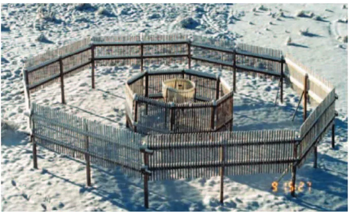
The DFIR consists of a large octagonal vertical double wind fence paired with a manually observed Tretyakov precipitation gauge. The diameters of the outer and inner fences of the DFIR are 12 and 4 m, respectively, installed at heights of 3.5 and 3 m, respectively (see Figs. 2 and 3). The top of the Tretyakov gauge in the center of the fence is level with the top of the inner fence. Wooden slats on both fences are spaced such that the porosity of the fence is 50%. This results in adequate gauge shelter from the wind but does not completely impede airflow. In all but the most extreme environments, drifting and blowing snow can move under the structure relatively unimpeded.
The DFIR configuration was extensively compared to a bush-sheltered Tretyakov gauge, considered to be a true representation of snowfall, at the hydrological research station near Valdai, Russia, from 1970 to 1990. Although the large octagonal double fence was shown to catch less snowfall than the bush gauge, the differences were relatively small (<10%) and could be corrected with the use of wind speed, pressure, temperature, and humidity measurements (Golubev 1989). This correction was later reassessed for vari-ous precipitation types (wet and dry snow, rain, and mixed) and simplified to use only wind speed (Yang et al. 1993). Although the bush gauge generally caught more snowfall than the DFIR, the WMO recognized that a man-made wooden structure would be more practical as a reference in a variety of climate regimes than a natural “bush” shield (Goodison et al. 1988). The Tretyakov gauge paired with the double fence has been the working standard for the manual measure-ment of precipitation in much of the former Union of Soviet Socialist Republics (USSR) since the late 1950s, and its performance has been well documented in a wide variety of conditions (Goodison et al. 1998; Yang et al. 1993).
Manual observations of snow mass in the DFIR gauge are typically made once or twice daily. These measurements are made volumetrically, as described previously, and have associated wetting losses. In recent years, automated gauges have replaced the manual gauge in the DFIR (Rasmussen et al. 2001).
There are several advantages and disadvantages to using the DFIR as a reference for the measurement of solid precipitation. The greatest advantage is the high catch efficiency of snowfall at moderate to high wind speeds. From Yang et al. (1993), the DFIR catch effi-ciency for dry snow remains greater than 90% at wind speeds (at gauge height) of 5 m s−1. At 8 m s−1, the CE
is still greater than 85%. Some of the disadvantages of this configuration include its large footprint, high cost of installation, and yearly maintenance. Also, the fence is effective at reducing the wind bias on the Tretyakov gauge inside, which can also inadvertently collect blowing snow and falsely increase CE during these events. Caution is required when using the DFIR as a reference during high wind events with blowing snow.
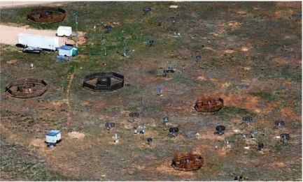
M A r s h A l l f i e l d s i t e t e s t B e d desCription. The Marshall Field Site is located 5 mi south of Boulder, Colorado, at an elevation of 1,700 m (39.950°N, 105.195°W) . This NCAR-owned field site is used to test and evaluate new and current meteorological instrumentation. The site is flat and level with semiarid grasses less than 0.25 m high. An aerial view of the site is shown in Fig. 4.
The National Oceanic and Atmospheric Adminis-tration (NOAA)/FAA/NCAR test bed was established at the Marshall Field Site in 1991. The establishment of this test bed was motivated by the need for real-time measurement of snowfall rate in support of aircraft ground deicing operations. Early studies at the test bed helped establish that the currently used technique to measure snow intensity via visibility is a poor estimate of the liquid equivalent snowfall rate (Rasmussen et al. 1999). An analysis of previ-ous ground deicing accidents suggested that liquid equivalent snowfall rate was underestimated during a number of these accidents (Rasmussen et al. 2000). This realization has sparked FAA-sponsored work regarding the development of a liquid equivalent sys-tem that can be used by airlines in support of ground deicing. A variety of gauges were tested at the site in support of this effort, including the development
Fig. 3. the dfir at Bratt’s lake, saskatchewan,
of a new precipitation sensor called the “hotplate” (Rasmussen et al. 2011).
The NOAA Climate Reference Network (CRN) program (www.ncdc.noaa.gov/crn/) has augmented the test bed infrastructure to evaluate a variety of gauges for use in measuring national precipitation trends, because accurate measurements of pre-cipitation are also necessary for quantifying climate change. To date, six different shield designs and four different gauges in various combinations have been tested at the Marshall Field Site test bed to determine the most accurate measure of the water content of solid precipitation using automated snow gauges for long-term climate measurements. Figures 5 and
6 show examples of single Alter– type and Tretyakov-type shields. Figure 7 presents a double Alter– type shield developed during the early 1990s at the Marshall Field Site (Rasmussen et al. 2001), and Fig. 8 shows an example of the DFIR shield. Figure 9 shows a series of hotplate precipitation gauges (Rasmussen et al. 2011), and Fig. 10 presents a Rosemount freezing rain sensor (currently sold by Campbell Scientific, Inc. 2010).
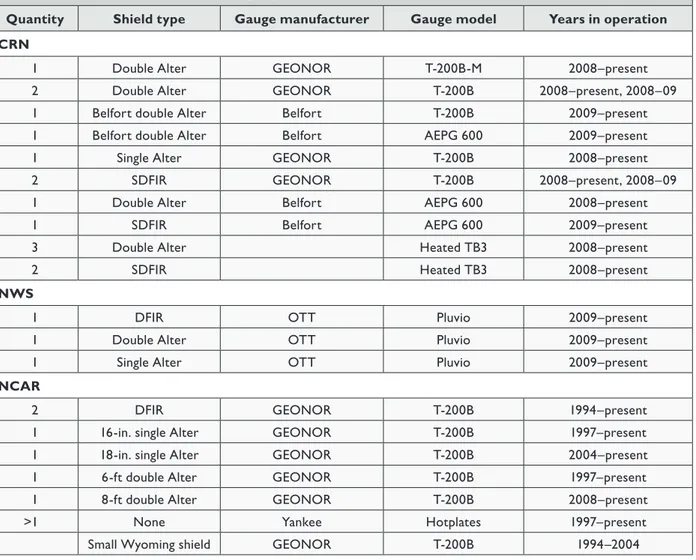
snoW gAuge And Wind-s h i e l d e v A l u At i o n studies. Specific gauges and wind shields tested. A list of the type of wind shields and gauge types tested at the site is given in Table 1. A DFIR shield has been present at the site since 1994, providing a long-term reference data-set for gauge intercomparison. All GEONOR gauges had heaters to prevent snow from accumulating on the walls (Hall and May 2004; Rasmussen et al. 2001). Most of the GEONORs had three vibrating wires for a redundant and more stable measurement. The AEPG 600 (Belfort Instrument, Maryland) gauge also utilized a three-wire weighing system. Load cell technolo-gies, such as the National Weather Service standard OTT Pluvio precipitation gauge (OTT Messtechnik, Germany), were also tested at the site. Tipping-bucket-type gauges (TB3, Hydrological Services PTY LTD, Australia) included a low-power heater (model TB323LP) activated by near-freezing air temperature (between +4° and −10°C) and the presence of snow in
Fig. 4. Aerial view of the Marshall field site. the three large shields
with two concentric fences in the top left are full-size dfir shields, and the two small dfir (sdfir) shields in the foreground with two concentric fences are two-thirds the size of the dfir shields. At the center of each sdfir is located a single Alter shield with a geonor snow gauge. smaller single and double Alter shields are located at various locations at the site. vegetation is less than 0.25 m tall.
Fig. 5. single Alter (left) and tretyakov shielded gauges
the gauge inlet. Hotplate precipitation gauges do not require a shield, and derive one-minute precipitation rates from measurement of the latent heat of evapora-tion and melting (Rasmussen et al. 2011).
Multiple installations of identical gauge/shield systems allow quantification of the accuracy and vari-ability of the precipitation measurements. All gauges are operated continuously, with data recorded every 60 s. A website was created to view the data in real time, to perform simple analyses, and to provide access to archived data (www.rap.ucar.edu/projects/winter/). Table 2 provides information on the power consump-tion of the various systems due to the heater operaconsump-tion. This information may be useful for remote site opera-tions, where access to power is limited.
The primary ancillary measurements included sonic temperature and three-dimensional wind speeds (YOUNG Model 81000, R. M. Young, Michigan) measured at a height of 7.38 m and recorded continuously at 10 Hz. Wind speed was also measured at a height of 1.5 m using a three-cup anemometer (model 014A, Met One, Oregon), and wind speed and wind direction were measured at a height of 9.2 m using a propeller anemometer (model 05103, R. M. Young). Air temperature was measured at a height of 1.5 m using six aspirated platinum resistance thermometers (Thermometrics, California).
Fig. 7. double Alter shield with geonor gauge in the
center at the Marshall field site.
Fig. 8. dfir shield with geonor in an Alter shield in
the center at the Marshall field site.
Fig. 9. Multiple hotplate precipitation gauges. in the
background (left) single Alter snow gauges and dfir shield.
Figure 11 shows the typical drop off in gauge col-lection efficiency as a function of wind speed for a double Alter-shielded gauge (Fig. 7). In this case, the standard measurement is an average of a small DFIR (SDFIR)-shielded GEONOR and full DFIR-shielded GEONOR (a SDFIR has a diameter of two-thirds of the normal DFIR and is the standard shield used by the U.S. Climate Reference Network). Note that the collection efficiency drops linearly from a value of 1.0 at 0 m s–1 to a value of 0.25 at 6 m s−1. Above 6 m s–1 the
collection efficiency tends to level out at ~0.25. The development of shield- and gauge-specific transfer functions, as shown by the “curvefit” in the figure, is necessary to correct for the undercatch of these gauges.
Also note the significant scatter in the measure-ments in Fig. 11 for a given wind speed. This is typically observed for all shield types and is likely due to the wide variety of snow crystal types and degrees of riming and aggregation, as well as varying turbulence intensity. Understanding and reducing
Table 1. description of the number, type of wind shield, manufacturer, precipitation gauge model, and
dates of operation of the precipitation gauges in operation at the test bed.
Quantity shield type gauge manufacturer gauge model Years in operation
Crn
1 Double Alter gEONOR T-200B-M 2008–present
2 Double Alter gEONOR T-200B 2008–present, 2008–09
1 Belfort double Alter Belfort T-200B 2009–present
1 Belfort double Alter Belfort AEPg 600 2009–present
1 Single Alter gEONOR T-200B 2008–present
2 SDFIR gEONOR T-200B 2008–present, 2008–09
1 Double Alter Belfort AEPg 600 2008–present
1 SDFIR Belfort AEPg 600 2009–present
3 Double Alter Heated TB3 2008–present
2 SDFIR Heated TB3 2008–present
nWs
1 DFIR OTT Pluvio 2009–present
1 Double Alter OTT Pluvio 2009–present
1 Single Alter OTT Pluvio 2009–present
nCAr
2 DFIR gEONOR T-200B 1994–present
1 16-in. single Alter gEONOR T-200B 1997–present
1 18-in. single Alter gEONOR T-200B 2004–present
1 6-ft double Alter gEONOR T-200B 1997–present
1 8-ft double Alter gEONOR T-200B 2008–present
>1 None Yankee Hotplates 1997–present
Small wyoming shield gEONOR T-200B 1994–2004
Table 2. typical precipitation gauge direct current power usage. heaters are controlled to maintain the
inlet temperature between 2° and 3°C when the air temperature is between –5° and 5°C, and precipitation is indicated by a wetness sensor. these measures help reduce power consumption, and they also prevent chimney effects and evaporation in the throat of the gauge caused by overheating.
Component power usage typical duty cycle
gEONOR T-200B 0.5 watts 24 h day−1
this scatter is an active area of research. Recent efforts have focused on the use of sonic anemometers to understand the airflow and turbulence around the gauges and to examine the collection efficiency as a function of crystal type as well as
airflow modeling. Developing an estimate of the scatter of the data (box plots, standard deviation) as a function of wind speed is another important characterization of each shield/gauge for users to understand the likely reliability of the given measurement.
Dependence of collection efficiency on shield type. A robust result from the past 15 years of gauge/shield testing is the consistently improved snow collection efficiency as one progresses from a single Alter shield, to a Tretykov shield, to a double Alter shield, to the two DFIR-type shields (small and standard) for the same gauge in the center of the shield. An example of this progression is shown in Fig. 12 from 23 to 24 March 2010. Note that the SDFIR and DFIR shields have the same accumulation, showing that one can use a smaller
version of the standard DFIR shield and still get excellent performance.
The single Alter-shielded gauge accumulates ~50% less precipitation than the same GEONOR gauge in the DFIR, showing the strong wind undercatch. The double Alter-shielded gauge is slightly better with ~55% undercatch. The most significant improvement is with the SDFIR, which is the same as the full DFIR. The hotplate snow gauge includes a wind correction factor, and in this particular event it overestimates precipitation compared to the DFIR by ~15%. These results clearly show that the wind shield is the most important factor for accurate snow measurement at various wind speeds.
Studies of airflow around the shields. fieLdstudies of theaiRfLowaRoundtheshieLdsusinGsonicdata. To
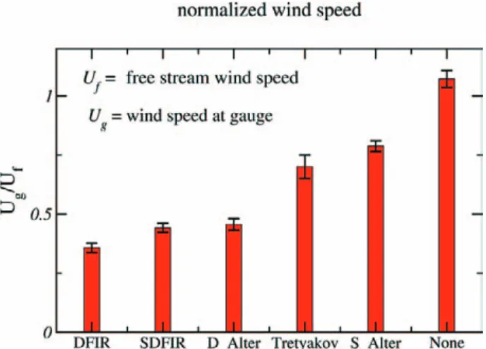
understand the behavior of the collection efficiency curves as given in Fig. 12, wind field studies have been conducted using sonic anemometers. The ver-tical velocity regime, as well as the reduction of the mean horizontal wind velocity at the gauge relative to that measured in nearby undisturbed flow condi-tions, showed a ranking that was consistent with the catch ratio results of Goodison et al. (1998) and the results reported here. For example, the gauge/shield configurations that resulted in the largest reduc-tion in the horizontal wind speed at the gauge inlet
Fig. 11. hourly catch ratios of solid precipitation vs
1.5-m height wind speeds. double Alter-shielded geonor measurements are normalized by the stan-dard hourly precipitation, which is the average of one sdfir- and one dfir-shielded geonor measure-ment. Best-fit linear “curvefit” (red line) is also shown with correlation coefficient.
Fig. 12. (left axis; upper plots) lWe accumulation (mm) during the
23–24 March 2010 snowstorm for a geonor gauge in a dfir, small dfir, double Alter, and single Alter wind shield. Also shown for comparison is the accumulation from a hotplate gauge and an ott pluvio 1 in a tretykov shield (right axis; lowest plot). Wind speed at 2 m in m s−1.
(Fig. 13) were also the gauge/shield configurations with the best CE (Figs. 14 and 15).
The results of the sonic study, which suggest that relative wind reduction at the gauge can be used as a surrogate for CE, were tested by examining a modi-fied double Alter (Belfort Instrument) with a 30% porosity compared to the standard 50% porosity. Wind speed reduction for the Belfort double Alter was significantly less than that of the standard con-figuration. Winter precipitation measurements from the Belfort double Alter confirmed improvements in catch relative to the double Alter and were nearly equal to the SDFIR measurements.
The schematic in Fig. 16 shows the relative size of the single, double, and DFIR shields and the reduction in flow velocity above each of the center points of each gauge–shield combination. Note the strong reduction in flow velocity over the DFIR shield as compared to the double and single Alter shields.
LaBoRatoRy and modeLinG studies of the aiRfLow aRoundshieLds. Wind tunnel tests demonstrate that
the airflow is deflected upward as the airstream ap-proaches an unshielded gauge orifice (Fig. 17). The various shields discussed in the previous section of the paper are designed to reduce this deflection and cause the airflow to flow more horizontally over the orifice, as it would over the ground. The reduction of the kinetic energy of the mean flow to turbulent ki-netic energy by the various shields effectively reduces the upward deflection through a reduced mean flow.
Figure 18 provides an example of a 3D computer model of snowflake trajectories past an unshielded gauge along the centerline of the gauge for an oncoming turbulent flow of 5 m s−1 and snowflake fall speed of 1 m s−1 (Thériault et al. 2012). The dashed lines are snowflake trajectories, and only the snow-flake that starts level with the gauge orifice upstream actually falls into the gauge due to the upward deflec-tion of the airflow by the gauge. If the airflow were more horizontal, as in the case of a shielded gauge, more of the snowflakes above the gauge orifice would have fallen into the gauge. In addition, the modeling study of Thériault et al. (2012) shows that the col-lection efficiency in a single Alter shield is strongly impacted by the snow crystal type.
snoW gAuge perforMAnCe during extreMe Winter WeAther Condi-tions: 17–19MArCh 2003 BlizzArd. On 17–19 March 2003, the Marshall Field Site experienced a blizzard. Winds were greater than 10 m s−1 for much of the event, and nearly 80 cm (30 in.) of
Fig. 13. reduction in wind speed at the center of a
shield as measured by sonic anemometers for various windshield types. Wind speed is nondimensionalized by the free stream value at gauge height.
Fig. 14. Ce for various types of wind shields relative to
the dfir. the geonor gauge was used for measuring the accumulation for all the shield types.
Fig. 15. Ce relative to the dfir from the WMo
inter-comparison test of solid precipitation using manual gauges.
snow accumulated on the ground by the time the storm was over (Fig. 19). This provided a unique opportunity to examine the performance of the various snow gauges under extreme winter conditions.
The liquid equivalent accumulation for this storm was ~120 mm during the 2.5-day event (Fig. 19). Note that there is no evi-dence of a “dump” of snow into any of the gauges due to the accumulation on the inner or outer sidewalls of the gauge (Fig. 19). This is attributed to the sidewall heating system
implement-ed into the upper portion of the GEONOR gauge to prevent capping (Fig. 20). The heater is only turned on if the temperature drops below 2°C.
The relative accumulation between the GEONOR gauges in the different wind shields is also shown in Fig. 19. Note that the single and double Alter-shielded gauges underestimated the snow accumulation by over 30% during this event. These results show the critical need to develop robust transfer functions that can correct for this type of undercatch. Because a signifi-cant fraction of annual snow accumulation can occur during these types of storms, it is imperative that the accumulation be correctly estimated. Climate models predict that winter storms will be more intense in the future. To verify this prediction, accurate and reliable measurements of snowfall rates and accumulations
for blizzards and other major winter storms will be needed. Proper shielding is clearly key to achieving the degree of accuracy necessary, which is one of the reasons why the CRN program has chosen to deploy a GEONOR in a two-thirds-diameter DFIR shield as its standard snow-measuring system.
The above discussion only applies to conditions with snow generated by natural cloud processes. During blowing snow conditions, special care needs to be taken to not overestimate snow accumulation due to wind effects alone.
Fig. 16. Airflow past precipitation gauges shielded by (a) single Alter, (b)
double Alter, and (c) dfir shields. Wind vectors are based on sonic anemom-eter measurements in fig. 13. top row of vectors represent free-stream wind speeds, and vectors immediately above the gauge (red) represent wind speeds measured at the gauge inlet.
Fig. 17. Mapping of airflow around a gauge orifice in
laminar wind tunnel flow.
Fig. 18. Airflow and snowflake trajectories past a
typi-cal snow gauge. oncoming airflow is 5 m s−1, and the fall speed of the simulated snowflake is 1 m s−1. Airflow
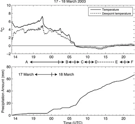
Video disdrometer observations of the 17–19 March 2003 blizzard. A video disdrometer was used to document the microphysical structure of the hydrometeors falling at the Marshall Field Site during the storm (Brandes et al. 2007). A time series of ambient tem-perature and dewpoint and liquid equivalent precipi-tation is shown in Fig. 21 for the first 40 h of the storm. The evolution of the hydrometeor terminal velocity, shape, and size distribution is shown in Fig. 22 as the storm transitioned from rain to mixed precipitation to all snow. Note the change in particle size distribution and fall velocity documented by the disdrometer as the storm transitions from rain to mixed phase to snow. AppliCAtion of snoW gAuges to AirCrAft deiCing: lWe sYsteM And CheCk tiMe. Aircraft deicing operations require real-time estimates of the liquid equivalent rate of pre-cipitation to estimate the length of time, called hold-over time, that a deicing fluid will be able to protect an aircraft from icing up. To address this need, the FAA directed NCAR to develop a real-time LWE system capable of providing accurate real-time estimates for snowfall rate every 5 min that could be deployed at an airport (Fig. 23). To achieve reliability and sufficient accuracy, three precipitation sensors were included: a GEONOR gauge in a single Alter shield, a hotplate snow gauge (Rasmussen et al. 2011), and a Vaisala PWD precipitation rate and type sensor. These three sensors
represent different technologies for measuring snow and complement some of the weaknesses inherent in each gauge. For instance, the PWD instrument estimates snowfall rate using an optical sensor. The hotplate estimates snowfall rate based on the cooling of a hotplate by the melting and sublimation of impacting snow on the top plate (Rasmussen et al. 2011). The GEONOR estimates snow mass using changes in frequency of a vibrating wire. Low snowfall rates less than 0.25 mm h−1 are estimated by the PWD sensor because it has a much lower onset threshold for snow detection and measurement than the other two sensors (hotplate and GEONOR typically need 0.25 mm h−1 with no wind to detect snow). The PWD also does not have a reduced collection efficiency under high wind conditions, so it is also used for snow-fall rate calculation when the winds are greater than 8 m s−1 and rates are less than 1 mm h−1 (at the typical gauge collection efficiency of 25%). For winds greater than 8 m s−1, 1 mm h−1 is needed to overcome the threshold rate for both the hotplate and GEONOR 5-min measurements.
In addition, the system uses the PWD sensor to es-timate precipitation type, and the Rosemount freezing rain sensor to determine the presence and rate of freezing rain and drizzle. Wind speed is measured
Fig. 19. liquid equivalent accumulation in the geonor in dfir,
sdfir, double Alter, and single Alter shields for the 17–19 Mar blizzard. Wind speed is given by the red line and is indicated by the scale on the right.
Fig. 20. heated geonor inside the dfir shield during
by the bottom plate of the hotplate due to its ability to remain ice free under icing conditions. A Vaisala WXT sensor is used to measure temperature and humidity and wind direction.
A new concept called check time has also been developed and tested at the Marshall Field Site test bed. Check time determines the fractional amount of aircraft deicing fluid holdover time expended each minute based on 1-min rate and temperature information from the LWE system and equations relating holdover time to precipitation rate. Once the sum of all the fractional holdover times reaches 1.0, the fluid is considered failed and the pilot needs to “check” the fluid on the wing for failure. This procedure allows the user to take into account the impact of time variations in rate and temperature on fluid holdover time.
The actual check time is a wall clock time in the past determined by subtracting the time needed for the fractional holdover time to reach 1.0 from the current wall clock time. If a pilot keeps track of the wall clock
time when he/she deiced, then one only needs to consult the wall clock check time to determine if the holdover time of the applied fluid has been exceeded. If the check time is before the time of deicing, then the fluid has not failed. If the check time is ahead of the time of deicing, then the fluid is considered failed, and the aircraft should be deiced again. The main advantage of check time is that only one wall clock time is needed for all aircraft on the field. An example of a check time display is shown in Fig. 24. neW Methods to MeAsure snoW. Cosmic ray–derived estimates of SWE. The intensity of low-energy cosmic ray neutrons is anticorrelated to the amount of hydrogen in soil or snow cover (Zreda et al. 2008; Desilets et al. 2010). Continuous measurements of neutrons using a dual-channel (fast and slow neutrons) cosmic ray probe placed a few meters above the surface can provide direct estimates of SWE within a 30–40-ha footprint (see Desilets et al. 2010 for details). In October 2010 a dual-channel CRS-1000 cosmic ray soil moisture probe from Hydroinnova LLC was installed as part of
the National Science Foundation–sponsored Cosmic Ray Soil Moisture Observing System (COSMOS 2010), a national network of soil moisture probes. Figure 25 shows the times series of the fast neutron counts from the Marshall Field Site test bed (Fig. 25a), cosmic ray–estimated SWE (Fig. 25b), and a snow water equivalent product whose inputs include hourly liquid water precipitation and sonic-ranging snow depth measurements (Fig. 25b). The COSMOS SWE retrieval was performed using an empirical calibration function obtained from simultaneous snow pillow and cosmic ray probe measurements at the Valles Caldera National Preserve in New Mexico. Neutron counting rates were corrected for temporal variations in barometric pressure and for changes in the baseline soil moisture level before and after each precipitation event. Figure 25c shows a plot of the COSMOS SWE and SWE estimates derived from manual measurements of snow depth and snow density during a 5-day storm period in late October 2009. The timing and magnitude of snow events and persistence of SWE from the two methods at the Marshall Field Site test bed are fairly consistent
Fig. 21. time series of (top) ambient temperature and dewpoint and
(bottom) liquid equivalent precipitation for the first 36 h of the storm. storm periods are labeled as follows: A: rain period, B: mixed-phase period, C: snow period with light–moderate riming, d: snow period with heavier riming, e: snow period with temperature above 0°C and small crystals, and f: snow period with temperature above 0°C and enhanced aggregation. no manual crystal observations were taken between 1235 and 1935 utC (dashed line).
Fig. 22. (top left) particle terminal velocity (m s−1) vs diameter, (bottom left) size distribution, and (right)
sample particle images from perpendicular directions for (a; facing page) the rain period (A), (b; facing page) the mixed-phase period (B), and (c) snow period (f).
Fig. 23. lWe display. Colored box at right provides the precipitation type by the background color (blue =
snow, green = rain, yellow = ice pellets, etc.), and the colored oval is the precipitation intensity: light (yellow), moderate (orange), and heavy (red). At top are site location, time (utC), temperature (°f), dewpoint (°f), rh (%), wind direction (true), wind speed (kt), liquid equivalent precipitation rate (mm h−1), precipitation trend over the last 10 min, temperature trend over the last 10 min, visibility (km), weather type, and precipitation intensity based on liquid equivalent rate (light, moderate, or heavy). graph is user selectable and shows the trend of the selected variable over the past hour.
effects. The overall Pearson correlation between the hourly NOAA CRN snow depth estimate and the COSMOS-derived SWE estimate is 0.87 and the root-mean-square error and mean biases are 5.1 and +2.4 mm, respectively. While work continues to further refine surface SWE and near-surface soil moisture measurements at the Marshall Field Site test bed, it is evident from these initial results that
Fig. 24. Check time display. Black vertical bar and white banner at top left indicates the check time for kifrost
ABC-s type iv anti-icing fluid with 100% concentration (wall clock time). Also indicated are the site location (Marshall), time, temperature, dewpoint, rh, wind direction, wind speed, precipitation rate (mm h−1), weather
type, last 10 min of the precipitation rate trend, last 30 min of the precipitation trend, and visibility (km). once the color bars change to red, the fluid has failed. Current time is on the far right of the display.
Fig. 25. CosMiC ray measurements of sWe at the
Marshall site. (a) hourly fast neutron counts, (b) CosMos-estimated (red) and Crn-derived (blue) snow Water equivalent (sWe), and (c) CosMos (circles), Crn (squares) and manual (triangles) mea-surements of sWe and snow depth (xs) during 27–31 oct. 2009. the bars on the manual measurements represent standard deviations of the samples collected during each measurement time.
despite significant differences in measurement scales, estimation assumptions, and local variations in snow cover due to wind redistribution and vegetation
the COSMOS system is capable of providing accurate and well-correlated SWE estimates at this semiarid, transient snowpack site.
GPS measurement of snow. Another method that can be used for large-scale measurement of snow on the ground comes from geodetic GPS sensors (Larson et al. 2009). Snow on the ground changes the por-tion of the GPS signal that reflects off of the ground surface (called multipath) and is received by a GPS antenna. This multipath signal interferes with the direct GPS signal, affecting the noise recorded in the combined GPS signal. As a GPS satellite rises, the lengths of the multipath and the direct path change at different rates, and as a result the two signals come in and out of phase with each other over time, causing the noise recorded by a GPS receiver to oscillate over time. The frequency of these oscillations is related to the height of the GPS antenna over the horizontal reflecting surface (Zavorotny et al. 2009), and this height changes with the height of the snow surface. The extent of this reflecting surface can be quite large, though it depends on the height of the GPS antenna above the ground. Most GPS antennas are installed approximately 2 m above the ground, leading to a surface reflection greater than 40 m long when the satellite is 5° above the horizon. Moreover, each GPS satellite follows a slightly different path, and a mea-surement can be made both when a satellite rises and when it sets. This leads to potentially 24 regions of the ground around the GPS antenna being measured every day, with additional measurements becoming available as the number of updated satellites in the GPS constellation increases.
A GPS receiver was installed at the Marshall Field Site test bed in late 2007 (Fig. 26). In the spring of 2009, two large snow events were observed at the Marshall Field Site, with approximately 30 and 35 cm of snow on the ground. The GPS record of snow depth correlates with the sonic snow depth record for these storms with a Pearson correlation of 0.91, and manual field measurements of snow depth suggest that the GPS sensor measures the field-average snow depth more accurately than the sonic snow depth measurements, largely because of the difference in measurement scales.
suMMArY And disCussion. This paper presents the NOAA/FAA/NCAR winter precipita-tion test bed located at the Marshall Field Site and some selected results from recent studies. Since the last WMO Intercomparison Test of Solid Precipita-tion (1989–93), new wind shields and new automated precipitation gauges have been developed. These wind shields and gauges have been the focus of studies con-ducted at this test bed for both real-time and climate time scales. The results show that while some progress has been made, measuring snow remains a significant challenge. Key challenges include the following: 1) Accounting for the reduction in snow catch due to
distortion of snowflake trajectories by the airflow pattern around a gauge. A number of wind shields have been created to reduce this effect, but no shield has yet been invented that has high collec-tion efficiency and is smaller than 4 m in diameter. 2) Eliminating snow capping on the gauge without
the use of significant amounts of heat.
Fig. 26. (a) gps antenna at the Marshall field site
during a snow event. (b) Comparison of snow depth
measurements over time made by manual measurements (black diamonds), automated ultrasonic instru-ments (grey lines), and the gps (red dots). the variation in the gps measureinstru-ments is caused partially by real spatial variability.
3) Reducing the minimum detectable signal below 0.2 mm h−1.
In most cases, deploying large wind shields, such as the DFIR, is either not possible or desirable, and thus simpler and smaller wind shields have been developed. However, our understanding of the fac-tors causing undercatch in the shields is not suffi-ciently well advanced to allow for the optimal shield design and only allows the development of empirical correction factors. Measuring and modeling the airflow around shield–gauge pairs has increased our understanding of the impact of wind shields on the airflow around the gauge. Future work will focus on understanding the impact of the airflow on the snow particles’ trajectories as well as the role of turbulence. Both field measurements and computer modeling studies are beginning to reveal some of the causes of the large scatter in the collection efficiency results.
Given the strong need for automated solid precipi-tation data from both the climate and weather com-munities, and the widely varying catch efficiencies of the various instruments, intercomparison studies are needed. The WMO-CIMO is organizing a Solid Precipitation Intercomparison Experiment (WMO-SPICE; www.wmo.int /pages/prog/www/IMOP /intercomparisons.html) focused on automatic pre-cipitation gauges and their configurations, in various climate conditions, building on the significant efforts currently underway in many countries. The aim of the intercomparison is to improve the understanding and reliability of solid precipitation measurements using automatic gauges, and will also include manual mea-surements using the standard defined by Goodison et al. (1998) for historical comparison. The study will take place starting in October of 2012 at sites around the world, including the United States, Norway, China, Canada, Japan, Switzerland, Russia, Finland and New Zealand. Any entities or vendors interested in participating in SPICE should contact their respec-tive national meteorological agency or the authors of this paper for further information.
The NOAA/FAA/NCAR precipitation test bed in Marshall, Colorado, in partnership with Envi-ronment Canada, collected data during the winter of 2011/12 to enable the WMO-SPICE organizing committee to determine the reference to be used by all other participants in 2012 for the measurement of solid precipitation. The NOAA/FAA/NCAR testbed has been chosen as one of the lead facilities for this study because of the comprehensive set of instrumentation in place for the measurement of solid precipitation.
ACknoWledgMents. This research was spon-sored by the National Science Foundation through an interagency agreement in response to requirements and funding by the Federal Aviation Administration’s Aviation Weather Research Program, the National Oceanic and Atmospheric Administration’s (NOAA) U.S. Climate Reference Network program administered at NOAA’s National Climatic Data Center (see www.ncdc.noaa.gov /crn/), and the U.S. Regional Climate Reference Network (USRCRN) program. The views expressed are those of the authors and do not necessarily represent the official policy or position of the U.S. government. The authors also acknowledge the support of Cheri Ward, program manager for the USRCRN and Jim Riley, the FAA contract manager for the NCAR ground deicing research and development effort. We also acknowledge the editing efforts by David L. Senn regarding the aerial site photo.
RefeRences
Alter, J. C., 1937: Shielded storage precipitation gauges.
Mon. Wea. Rev., 65, 262–265.
Brandes, E., K. Ikeda, G. Zhang, M. Schönhuber, and R. M. Rasmussen, 2007: A statistical and physical description of hydrometeor distributions in Colorado snow storms using a video disdrometer. J. Appl.
Meteor. Climatol., 46, 634–650.
Campbell Scientific, Inc., cited 2010: SR50A sonic rang-ing sensor. [Available online at www.campbellsci.ca /Catalogue/SR50A_Man.pdf.]
Desilets, D., M. Zreda, and T. P. A. Ferré, 2010: Nature’s neutron probe: Land surface hydrology at an elusive scale with cosmic rays. Water Resour. Res., 46, W11505, doi:10.1029/2009WR008726.
Erickson, T., M. W. Williams, and A. Winstral, 2005: Persistence of topographic controls on the spatial distribution of snow depth in rugged mountain terrain, Colorado, United States. Water Resour. Res.,
41, W04014, doi:10.1029/2003WR002973.
Fischer, A. P., 2011: The measurement factors in esti-mating snowfall derived from snow cover surfaces using acoustic snow depth sensors. J. Appl. Meteor.
Climatol., 50, 681–699.
Golubev, V. S., 1989: Assessment of accuracy charac-teristics of the reference precipitation gauge with a double-fence shelter. Final Report of the Fourth Session of the International Organizing Committee for the WMO Solid Precipitation Measurement Intercomparison, 22–29.
Goodison, B. E., 1978: Accuracy of Canadian snow gage measurements. J. Appl. Meteor., 17, 1542–1548. —, and D. Yang, 1996: In-situ measurements of
correction. Proceedings of the Workshop on the ACSYS Solid Precipitation Climatology Project, WMO/TD-739, WCRP-93, 3–17.
—, J. R. Metcalfe, and R. A. Wilson, 1988: Devel-opment and performance of a Canadian auto-matic snow depth sensor. WMO Instruments and Observing Methods Rep. 33, 317–320.
—, P. Y. T. Louie, and D. Yang, 1998: WMO solid precipitation measurement intercomparison. WMO Instruments and Observing Methods Rep. 67, WMO/ TD-872, 212 pp.
Groisman, P. Ya., and D. R. Legates, 1994: The accu-racy of United States precipitation data. Bull. Amer.
Meteor Soc., 75, 215–227.
Gultepe, I., and J. A. Milbrandt, 2010: Probabilistic parameterizations of visibility using observations of rain precipitation rate, relative humidity, and vis-ibility. J. Appl. Meteor. Climatol., 49, 36–46. Hall, M. E., and E. May, 2004: Inlet heater for USCRN
weighing precipitation gauge. NOAA Tech. Note NCDC USCRN-04-01, 10 pp. [Available at www .ncdc.noaa.gov/crn/docs.html.]
IPCC, 2007: Climate Change 2007: The Physical Science
Basis. Contirbution of Working Group I to the Fourth Assessment Report of the Intergovernmental Panel on Climate Change. Cambridge University Press, 996 pp.
Jenoptik, cited 2012: Snow depth sensor SHM 30: A compact laser senor for determining snow depths. [Available online at www.weatherlife.co.kr/catalog /shm_30_en_web.pdf.]
Larson, K. M., E. E. Small, E. D. Gutmann, A. L. Bilich, J. J. Braun, and V. U. Zavorotny, 2008: Use of GPS receivers as a soil moisture network for water cycle studies. Geophys. Res. Lett., 35, L24405, doi:10.1029/2008GL036013.
—, E. D. Gutmann, V. U. Zavorotny, J. J. Braun, M. W. Williams, and F. G. Nievinski , 2009: Can we measure snow depth with GPS receivers? Geophys. Res. Lett.,
36, L17502, doi:10.1029/2009GL039430.
Larson, L. W., 1993: ASOS heated tipping bucket precipi-tation gage (FRIEZ) evaluation at WSFO, Bismarck, North Dakota, March 1992-March 1993. NWS Central Region Final Rep., 54 pp.
McKee, T. B., N. J. Doesken, C. A. Davey, and R. A. Pielke, Sr., 2000: Climate data continuity with ASOS: Report for period April 1996 through June 2000. Climatology Rep. 00–3, Colorado Climate Center, Colorado State University, 82 pp.
Metcalfe, J. R., and B. E. Goodison, 1993: Correction of Canadian winter precipitation data. Proc. Eighth
Symp. on Meteorological Observations and Instru-mentation, Anaheim, CA, Amer. Meteor. Soc.,
338–343.
Nitu, R., and K. Wong, 2010: CIMO survey on national summaries of methods and instruments for solid precipitation measurement at automatic weather sta-tions. WMO Instruments and Observing Methods Rep. 102, WMO/TD-1544, 57 pp. [Available online at www.wmo.int/pages/prog/www/IMOP/publications /IOM-102_SolidPrecip.pdf.]
Rasmussen, R. M., J. Vivekanandan, J. Cole, B. Myers, and C. Masters, 1999: The estimation of snowfall rate using visibility. J. Appl. Meteor., 38, 1542–1563. —, J. Cole, K. R. K. Moore, and M. Kuperman, 2000:
Common snowfall conditions associated with air-craft takeoff accidents. J. Airair-craft, 37, 110–116. —, and Coauthors, 2001: Weather support to deicing
decision making (WSDDM): A winter weather nowcasting system. Bull. Amer. Meteor. Soc., 82, 579–595.
—, J. Hallett, R. Purcell, and S. Landolt, and J. Cole, 2011: The hotplate precipitation gauge. J. Atmos.
Oceanic Technol., 28, 148–164.
Sevruk, B., and S. Klemm, 1989: Catalogue of national standard precipitation gauges. WMO Instruments and Observing Methods Rep. 39, WMO/TD-313, 50 pp.
—, J.-A. Hertig, and R. Spiess, 1991: The effect of precipitation gauge orifice rim on the wind field deformation as investigated in a wind tunnel. Atmos.
Environ., 25A, 1173–1179.
Smith, C. D., 2009: The relationship between snowfall catch efficiency and wind speed for the Geonor T-200B precipitation gauge utilizing various wind shield configurations. Proc. 77th Western Snow
Con-ference, Canmore, AB, Canada, 115–121.
Thériault, J., R. Rasmussen, K. Ikeda, and S. Landolt, 2012: Dependence of snow gauge collection effi-ciency on snowflake characteristics. J. Appl. Meteor.
Climatol., 51, 745–762.
Yang, D., J. R. Metcalfe, B. E. Goodison, and E. Mekis, 1993: “True snowfall”: An evaluation of the double fence intercomparison reference gauge. Proc. 50th
Eastern Snow Conference/61st Western Snow Confer-ence, Quebec City, QC, Canada, 105–111.
Zavorotny, V., K. M. Larson, J. Braun, E. E. Small, E. D. Gutmann, and A. Bilich, 2009: A physical model for GPS multipath caused by land reflections: Toward bare soil moisture retrievals. IEEE J. Sel. Top. Appl.
Earth Obs. Remote Sens., 3, 100–110, doi:10.1109/
JSTARS.2009.2033608.
Zreda, M., D. Desilets, T. P. A. Ferré, and R. L. Scott, 2008: Measuring soil moisture content non-invasively at intermediate spatial scale using cosmic-ray neutrons. Geophys. Res. Lett., 35, L21402, doi:10.1029/2008GL035655.