https://doi.org/10.1007/s00429-020-02046-1
METHODS PAPER
CBPtools: a Python package for regional connectivity‑based
parcellation
Niels Reuter1,2 · Sarah Genon1,2 · Shahrzad Kharabian Masouleh1,2 · Felix Hoffstaedter1,2 · Xiaojin Liu1,2 ·
Tobias Kalenscher3 · Simon B. Eickhoff1,2 · Kaustubh R. Patil1,2 Received: 13 September 2019 / Accepted: 8 February 2020
© The Author(s) 2020
Abstract
Regional connectivity-based parcellation (rCBP) is a widely used procedure for investigating the structural and functional differentiation within a region of interest (ROI) based on its long-range connectivity. No standardized software or guidelines currently exist for applying rCBP, making the method only accessible to those who develop their own tools. As such, there exists a discrepancy between the laboratories applying the procedure each with their own software solutions, making it dif-ficult to compare and interpret the results. Here, we outline an rCBP procedure accompanied by an open source software package called CBPtools. CBPtools is a Python (version 3.5+) package that allows users to run an extensively evaluated rCBP analysis workflow on a given ROI. It currently supports two modalities: resting-state functional connectivity and structural connectivity based on diffusion-weighted imaging, along with support for custom connectivity matrices. Analysis parameters are customizable and the workflow can be scaled to a large number of subjects using a parallel processing environment. Par-cellation results with corresponding validity metrics are provided as textual and graphical output. Thus, CBPtools provides a simple plug-and-play, yet customizable way to conduct rCBP analyses. By providing an open-source software we hope to promote reproducible and comparable rCBP analyses and, importantly, make the rCBP procedure readily available. Here, we demonstrate the utility of CBPtools using a voluminous data set on an average compute-cluster infrastructure by performing rCBP on three ROIs prominently featured in parcellation literature.
Keywords Connectivity-based parcellation · Clustering · Resting state · Diffusion-weighted imaging · Software
Introduction
Mapping the human brain in an effort to understand its organizational principles is a monumental task, dating back to the early 1900s with Korbinian Brodmann’s famous publication on ’Vergleichende Lokalisationslehre der Großhirnrinde’ (Localization in the cerebral cortex; Brod-mann (1909)). The advent of modern non-invasive in vivo neuroimaging technologies, such as magnetic resonance imaging (MRI), has been driving growth in this research field. Accompanying progress in neuroimaging data analy-sis techniques allow a range of connectivity measurements from various MRI modalities. Brain organization can then be probed by analyzing the patterns in these measurements. One such technique is connectivity-based parcellation (CBP), an umbrella term for a widely used and diverse set of procedures to delineate whole- and regional brain organi-zation, originally conceived by Behrens et al. (2003) in their seminal work on the thalamus.
This study was supported by the European Union’s Horizon 2020 Research and Innovation Programme under Grant Agreement no. 785907 (HBP SGA2) and Grant Agreement no. 7202070 (HBP SGA1). SG was partly supported by the Deutsche Forschungsgemeinschaft (DFG) under Grant Agreement GE 2835/1-1.
Electronic supplementary material The online version of this article (https ://doi.org/10.1007/s0042 9-020-02046 -1) contains supplementary material, which is available to authorized users. * Kaustubh R. Patil
1 Institute of Systems Neuroscience, Heinrich-Heine University, Düsseldorf, Germany
2 Institute of Neuroscience and Medicine, Brain and Behaviour (INM-7), Research Centre Jülich, Jülich, Germany
3 Comparative Psychology, Institute of Experimental Psychology, Heinrich-Heine University Düsseldorf, Düsseldorf, Germany
A common approach to mapping the human brain through CBP is to cluster voxels/vertices into parcels. Here, we focus on regional CBP (rCBP). A clustering algorithm is used to group voxels/vertices within a given region of interest (ROI) based on similarity in their connection strengths to a set of target voxels/vertices, i.e., their connectivity profile. Voxels clustered together form homogeneous units, i.e., par-cels, with regard to the measured connectivity marker that best describes the input data at hand. The parcels are often spatially consistent, as neighboring voxels usually exhibit more similar connectivity patterns than those further away. Thus, the rCBP procedure can map functional or structural subdivisions/clusters within a particular ROI. rCBP derived parcels are known to match with histological parcellation (Bzdok et al. 2013), but they may also provide subdivisions pertaining to different sources of information not revealed by cytoarchitectonic mapping alone (Clos et al. 2013). As each MRI modality yields a different aspect of brain con-nectivity, rCBP on each modality can yield differing parcel-lations with different interpretations. Commonly used imag-ing modalities include, but are not limited to, restimag-ing-state blood oxygen level-dependent (BOLD) time series used to measure task-independent functional connectivity and diffu-sion-weighted imaging (DWI)-based probabilistic diffusion tractography to estimate anatomical fiber connectivity, as well as meta-analytic connectivity modeling (MACM) as a measure of task-dependent functional connectivity and co-activation patterns. Due to the different interpretations that may result from each modality, a multimodal approach [e.g., Genon et al. (2018) and Plachti et al. (2019)] may be used to compare unimodal parcellations.
Various methods can be employed at different steps within the rCBP procedure. For instance, unlike whole-brain parcellations (Schaefer et al. 2018), rCBP focuses on a particular ROI, hence allowing an in-depth analysis by uncovering the internal differentiation of a region. Our approach relies on using static rather than dynamic (Hutch-ison et al. 2013; Ji et al. 2016) patterns of connectivity. Moreover, we use a hard cluster assignment employing an unsupervised machine learning algorithm (k-means, spec-tral, or agglomerative clustering) as opposed to probabilistic, graded (Bajada et al. 2017), or boundary mapping (Cohen et al. 2008) approaches. For a more detailed overview of the rCBP procedure, we recommend reading Eickhoff et al. (2015) and Eickhoff et al. (2018).
Despite its popularity, rCBP is challenging and time con-suming to employ without the necessary tools. As neuro-science makes a transition toward big data, with prominent examples such as the Human Connectome Project (HCP) (Van Essen et al. 2013) and the 1000BRAINS study (Caspers et al. 2014) having well over 1000 subjects, it becomes an increasing necessity to add support for high-throughput computation and parallel processing. Furthermore, the
numerous options available at each step of the rCBP proce-dure paired with the absence of uniform guidelines make it difficult to have comparable results. For example, the choice of clustering algorithm may influence the clustering results, with options such as k-means clustering, spectral clustering, or hierarchical clustering (Hastie et al. 2013; Von Luxburg
2007).
To resolve these issues, we introduce CBPtools, an open-source distributed workflow for rCBP enclosed in a Python package. By unifying the methodological choices behind the procedure into a customizable workflow, we offer a fast, sta-ble, and reproducible means to parcellate the brain regions. Furthermore, computational demands highlighted by com-plex algorithms and large data sets are mitigated by efficient parallel execution of the procedure. CBPtools offers a com-mon working ground to effortlessly and efficiently conduct reproducible and data-driven parcellation analyses.
Materials and methods
CBPtools overview
CBPtools parcellates an ROI and provides the output as
NIfTI images along with commonly used cluster-validity metrics. The tool’s approach and methods are derived from a substantial body of parcellation works (Wang et al. 2015; Bzdok et al. 2015; Chase et al. 2015; Barron et al. 2015; Hardwick et al. 2015; Eickhoff et al. 2016; Muhle-Karbe et al. 2016; Genon et al. 2017, 2018; Plachti et al. 2019) and consist of a customizable rCBP workflow allowing users to specify the input data and a range of parameters through a configuration file. CBPtools can calculate con-nectivity matrices from resting-state or DWI data, but they may instead be provided directly as input. It then computes parcellations based on the connectivity matrices (projected onto NIfTI images of the ROI and as NumPy array files, as well as 3D voxel plots) and outputs validity metrics for their evaluation. Note that the procedure outlined here utilizes hard clustering. Therefore, when connectivity markers are assumed to change through soft transition (i.e., showing a gradient), parcels generated through this procedure should not be interpreted as neurobiological units, but as a simpli-fied data representation (or compression model). Figure 1
provides an overview of the workflow procedure, with each step detailed in the following sections.
To illustrate both the usage of CBPtools and the output it provides, the resting-state and DWI modalities of the HCP data (Van Essen et al. 2013) were used to parcellate three regions that have been frequently analyzed using the rCBP procedure: the right (R) Insula, R amygdala, and an ROI comprising R presupplementary motor area (preSMA) and
R supplementary motor area (SMA) (see "Example data" for details).
Architecture
CBPtools is written in Python (version 3.5+) to exploit
Python’s prolific presence in the data science community and can be installed with pip (‘pip install cbptools’). We capitalized on pre-existing and widely used packages, such as NumPy, SciPy, NiBabel, and scikit-learn, which provide a range of methods needed for the rCBP procedure. This makes the software very accessible on account of Python and its libraries being free and open source, as well as com-patible with many operating systems.
CBPtools makes use of snakemake (Köster and
Rah-mann 2012), an easy-to-use and well documented work-flow management system with parallel processing capa-bilities that allows the workflow execution to be scaled to various processing environments (i.e., server, cluster, grid, or cloud environments). Through snakemake,
CBP-tools is compatible with job schedulers that support shell
script (such as SLURM and qsub). Furthermore, CBPtools can be resumed with partially processed data (e.g., due to hardware failure) making it stable and efficient for use on real world data. The combination of snakemake’s com-mand line execution and an easily modifiable configuration file make it possible to set up and run the software without any programming knowledge.
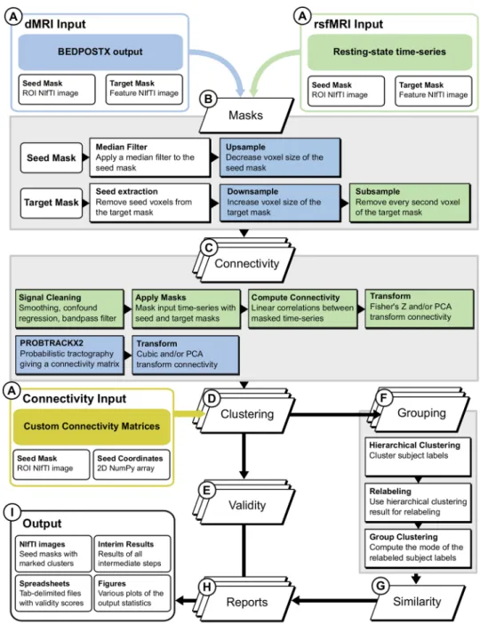
Fig. 1 CBPtools workflow for
applying the rCBP procedure to diffusion MRI (dMRI) or resting-state functional MRI (rsfMRI) data. After customiz-ing the parameters of the proce-dure, input data (A) is processed through each step (B through H) of the workflow. Note that the different types of inputs are not processed in parallel, but must instead be set up and executed as different CBPtools projects. Steps are executed in parallel whenever possible (e.g., the connectivity, clustering, valid-ity, grouping, and reports steps). The mask preprocessing and connectivity steps use differ-ent methods based on the input modality (i.e., dMRI or rsfMRI, highlighted in blue and green, respectively). Thus, methods with a green background are only performed on rsfMRI data, and methods with a blue background are only performed on dMRI data. Alternatively custom connectivity matrices can be given as input, which will skip steps B and C
For a more detailed instruction on the use of the package, please visit the repository at https ://githu b.com/inm7/cbpto ols or our online documentation (Reuter 2019).
Setup and input specification
Processing parameters and options can be defined by means of a configuration file, for which the parameter choices and fields will be validated and logged. Errors during the setup must first be resolved before proceeding, but warnings are not critical to the execution of CBPtools. However, they may give rise to unexpected results and should not be ignored. Upon completion of the setup, a new project folder is created at a user-specified location, containing all files necessary to initiate the workflow. The CBPtools online documentation (Reuter 2019) has a more detailed overview of the setup process. We have also provided a quick-start guide in the Online Resource (Sect. 1.2 Usage example) as well as on the GitHub project page.
The input data are separated into modality-independent and modality-dependent categories. Modality-independent input data include (1) a binary three-dimensional NIfTI ROI file in the three-dimensional NIfTI image data format, (2) an optional three-dimensional target mask in the same data format, used to define the connections that are considered for each ROI voxel. If not provided by the user, the FSL (http://www.fmrib .ox.ac.uk/fsl/) distributed average Mon-treal Neurological Institute (MNI) 152 T1 whole-brain gray matter group template (2 mm isotropic) will be used as the target, in which case the required input data should match the same MNI152 template as well, and (3) a participants file as a tab-separated text file with a column called
‘partici-pant_id’ containing all unique identifiers of the subjects to
be included in the study.
Modality-dependent data depend on the selected input modality, i.e., rsfMRI, dMRI, or connectivity. For rsfMRI data, a 4D time series NIfTI image per subject must be pro-vided, optionally accompanied by a tab-separated text file containing confounds for each time point as columns.
CBP-tools assumes that the rsfMRI data have been treated with
necessary fMRI preprocessing including realignment and normalization to a template space. If the default target mask is used, then the template space must be MNI152 with 2 mm isotropic voxels. CBPtools also supports using native masks, but that prohibits the use of the default mask (for more information, see Online Resource Sect. 1.3.3 Single-subject parcellation). Denoising based on independent com-ponent analysis like Automatic Removal of Motion Artifacts (ICA-AROMA) (Pruim et al. 2015) or FMRIB’s ICA-based X-noiseifier (FIX) (Salimi-Khorshidi et al. 2014) is encour-aged if suitable. In particular, FIX in combination with mean white matter and cerebrospinal fluid signal regres-sion has been shown to work well in the context of rCBP
(i.e., improved cluster stability and consistency of clusters between neuroimaging modalities) (Plachti et al. 2019). The dMRI modality requires input necessary to perform FSL’s probabilistic diffusion tractography (PROBTRACKX2), consisting of: (1) outputs from Bayesian estimation of diffu-sion parameters obtained using sampling techniques (BED-POSTX), (2) a brain extraction (BET) binary mask file, (3) a transform file taking seed space to DTI space (either a FLIR matrix or FNIR warpfield; optional), and (4) a file describing the transformation from DTI space to seed space (optional unless input file 3 is defined). Each of these files is subject specific and can be obtained from FSL’s BEDPOSTX out-put. Connectivity matrices may be provided as source input in lieu of rsfMRI or dMRI data. They must be provided in a ROI-voxel by target-voxel shape, along with a binary three-dimensional mask of the ROI in NIfTI image data format, and a NumPy array of voxel coordinates in the order that the ROI voxels are represented in the connectivity matrix.
To define input data for the rCBP procedure, the full file paths must be added to the configuration file. CBPtools offers example configuration files using the ‘cbptools
exam-ple–get data-type’ command, where data type is replaced
by either ’connectivity’, ’rsfmri’, or ’dmri’, reflecting the different input data types. The absolute file path for subject-wise files should be specified as a template, i.e., containing the string {participant_id} which will be replaced by the ids of the subjects included in the rCBP project (through the inclusion of the aforementioned participant’s file). All input data should be quality controlled prior to using CBPtools, as only marginal validation is performed on the input data by
CBPtools. Faulty data may halt processing until the issues
are resolved, but in the worst case such data may provide output without explicit warnings that this output should not be trusted. Further specified during the setup are parameters to transform the connectivity matrices (e.g., cubic or Fisher’s
Z transform, or feature reduction through principal
compo-nent analysis), the clustering parameters (e.g., the range of
k clusters requested) and validity measures, as well as the
desired output file formats. Each of these parameters are likewise specified in the configuration file.
ROI mask preprocessing
There are various atlases and tools that can be used to respectively define an ROI and extract it as a binary mask. For instance, the JuBrain Anatomy Toolbox (Eickhoff et al.
2005) can be utilized to extract an ROI using probabilistic cytoarchitectonic maps. Alternatively, the FSL distributed atlases (e.g., the Harvard-Oxford Atlas) can likewise be used to extract an ROI. The mask must be a three-dimensional binary NIfTI image.
The ROI mask is validated for binarity and conformity to either an optionally provided target mask, or by default
the group MNI template space (2 mm isotropic voxels, 91 × 109 × 91 shape, and origin at x = 90, y = − 126 , z = − 72 ). When connectivity matrices are given as input in lieu of rsfMRI or dMRI data, the ROI mask is only validated for binarity. For all other cases, it is important that input data are in the same space as the mask. It is possible to use a different space, but then a target mask must be provided in the desired space, which then both the ROI mask and input data must conform to. Without a user-provided target mask, all whole-brain gray mat-ter voxels are used as target and subsampled (see below) by default (although this option can be turned off in the configuration file).
Available preprocessing steps are modality specific and all are optional. For the rsfMRI modality, the ROI mask can be median filtered and the target mask can be subsampled and have all ROI voxels removed from it. Median filtering replaces each voxel with the median of its neighboring voxels. For binarized images, this will remove voxels with too few neighbors and add voxels to the mask when they have many neighbors. It can be par-ticularly useful for hand-drawn ROIs, as it removes sharp borders or stray voxels that would not naturally occur in most ROIs. Subsampling the target mask is recommended when smoothed BOLD time series are used. This means that only every second voxel in each dimension is kept under the spatial-smoothness assumption that neighbor-ing voxels provide a relatively similar signal. This can significantly reduce computation time while preserving most of the information due to spatial smoothness. By choosing to remove all ROI voxels from the target mask, the ROI to ROI (i.e., within-ROI) connectivity is ignored. Within-ROI connectivity (i.e., connectivity between every pair of voxels within the ROI) tends to be high due to their relative proximity to one another and may there-fore dominate the clustering. Whether doing so leads to better or more biologically relevant parcellation results, however, is unclear. Its application can also optionally remove a border around the ROI to reduce the influence of smoothing. For dMRI, in addition to median filtering, the ROI can also be upsampled. This upsampling option spreads the ROI voxels to cover a larger area (reflect-ing a higher resolution for use with PROBTRACKX2), while maintaining the same number of voxels (which is necessary so that ROI voxels can be mapped back upon the original ROI mask). Thus, voxels within the upsam-pled ROI will be spread out equidistantly over a larger area with no direct neighboring voxels as a result of not increasing their amount. The target mask can be down-sampled from a higher to a lower resolution, resulting in fewer voxels covering the same space (i.e., larger voxels) which can reduce computation time for PROBTRACKX2.
Connectivity computation
To derive rsfMRI connectivity, the BOLD time series are optionally smoothed [using NiBabel’s (Brett et al. 2019)
nib-abel.processing.smooth_image], nuisance signal regressed
(linear regression of confound time points on subject time series), and band-pass-filtered. An ROI-to-target connectiv-ity matrix is calculated per subject using linear correlations between the ROI and target BOLD time series. A user can optionally choose for the connectivity matrices to be Fisher’s
Z transformed and/or be subjected to linear
dimensional-ity reduction (through principal component analysis). For dMRI, the PROBTRACKX2 output, a sparse ROI- by target-voxel connectivity matrix (omatrix2) per subject, is densified and cubic transformed, and can optionally be subjected to linear dimensionality reduction as well.
Individual‑ and group‑level clustering
Connectivity from the previous step is given as input to the
k-means algorithm [using scikit-learn’s (Pedregosa et al. 2011) sklearn.cluster.KMeans], separately for each subject and for each requested number of clusters k. Alternatively, agglomerative/hierarchical (Hastie et al. 2013) or spec-tral clustering (Von Luxburg 2007) can be used instead of
k-means. The k-means algorithm was chosen as the default
algorithm due to its popularity in CBP literature. The clus-tering algorithm assigns each ROI voxel/vertex to a cluster, effectively grouping similar voxels based on their connec-tivity profiles (for k-means this is done by minimizing the squared Euclidean distance between voxel features, i.e., the connectivity profiles and that of cluster centers). Thus, for each individual subject and a given modality, the output is the parcellation of the ROI voxels/vertices.
As the individual-level cluster ids are arbitrary, to deter-mine a group parcellation that best describes all included subjects first, the individual clusterings at each k are rela-beled such that similar clusters get assigned the same cluster ids across subjects. For each k, all individual clusterings are given as input to SciPy’s (Jones et al. 2001) implementation of hierarchical clustering (scipy.cluster.hierarchy) using the Hamming distance metric and a user-defined linkage algo-rithm (defaults to ’complete’). Hamming distance is used to take the arbitrary nature of the cluster ids into account. The hierarchical clustering result serves as a reference for rela-beling individual clusterings (Nguyen and Caruana 2007). Relabel accuracy is calculated for each subject to identify the permutation of cluster ids that most accurately reflects the match of a given clustering with the reference cluster-ing. Relabel accuracy is also presented as one of the various validity metrics (for more information see Online Resource Sect. 2.4 Relabeling strategy). Next, the mode of the rela-beled subject-wise clustering is computed and used as the
group-level clustering. Optionally, the hierarchical cluster-ing result can be used as a group-level clustercluster-ing in lieu of the mode group-level clustering. Subject-wise follow-up analyses done in subsequent steps refer to the individual clusterings, and group analyses refer to the group-level clus-tering. Note that the group-level parcellation is not calcu-lated when parcellation is performed in the native space. Clustering validity
Finding the appropriate number of clusters is a challenging and unresolved problem. It is common to probe a range of
k values starting at two to a number determined through
prior knowledge of the ROI and the source data (i.e., based on modality, granularity of the data, or the selected target regions) structure. Therefore, the clustering solutions at different k need to be evaluated. One possibility is using external validation, which contrasts the clustering solutions against a predetermined structure which is independent of the source data (i.e., using a predefined cytoarchitectonic parcellation as an external reference for clustering the results of the same region). In the absence of information for exter-nal validation (as is frequently the case), interexter-nal cluster validation can help to select an optimal clustering in a data-driven way. Several such metrics can be used to rank the clustering results. However, different metrics often produce divergent results. Baarsch and Celebi (2012) evaluated the Dunn index, the Davies–Bouldin index, the Calinski–Hara-basz index, the Silhouette index, the point biserial measure, the Pakhira–Bandyopadhyay–Maulik (PBM) score, and sum-of-squares. They concluded sum-of-squares to be most effective, closely followed by the Silhouette index. Popular alternatives like the Davies–Bouldin index and the Calin-ski–Harabasz index were only moderate contenders, while the Dunn index performed poorly. Even the best measure, however, was only correct in 60% of the test cases. Neverthe-less, validity metrics are often tested on simulated or simple data sets which might not generalize to the complexity inher-ent in the connectivity data. Furthermore, there exist many more validity metrics [such as the I index, which was tested to perform well in a review by Maulik and Bandyopadhyay (2002)]. In general, it is difficult to deem any single valid-ity metric to be good for clustering, as data properties may vary significantly between data sets. Therefore, CBPtools provides several validity metrics and sufficient care must be given when deciding which measure to rely upon, also evident from our results.
Validity metrics and report
Clustering outputs the solution for each clustering granular-ity k both separately for each subject and grouped together into a group-level clustering. For each individual clustering
at each value of clustering granularity k, several cluster qual-ity metrics can be obtained. These include: the Silhouette index (Rousseeuw 1987), the Calinski–Harabasz index (Cal-inski and Harabasz 1974), and the Davies–Bouldin index (Davies and Bouldin 1979). For group labels, again for each
k, relabel accuracy and cophenetic correlation, as a measure
on how well the pairwise distances between the individual cluster labels are preserved in the group-level clustering, are given. Similarity between individual clusterings can also be examined based on the Adjusted Rand index (Rand 1971; Hubert and Arabie 1985), the V measure (Cramér 1946), or the adjusted mutual information (Vinh et al. 2010) scores (whichever is chosen by the user). The resulting similarity matrices, showing the similarity between pairs of individual subject clusterings for each k, are presented as dendrograms. Likewise, similarity between individual clusterings to the group clustering is computed using the same metric. Care needs to be taken when interpreting this score, however, since the group-level clustering is not independent of the individual subject clusterings which might inflate similarity scores. Lastly, the group clustering is mapped upon the ROI mask and stored as an NIfTI image which can be visualized using any of the various NIfTI format image viewers [e.g., Mango (http://ric.uthsc sa.edu/mango /), MRIcron (https :// www.nitrc .org/proje cts/mricr on) or FSLeyes (https ://fsl. fmrib .ox.ac.uk/fsl/fslwi ki/FSLey es)].
The statistics are stored as tab-separated files as well as figures in a user-defined file format. Interim data (e.g., connectivity, cluster labels) are stored as NumPy (Oliphant
2006) binary files and tab-separated text files. This data can then be used to determine what cluster solution best fits the input data, and hence is best suited for further use in more in-depth analyses. Optionally, subject-specific reports (i.e., metrics and plots) can be obtained in addition to the group-level clustering reports if specified in the configuration file (see Online Resource Sect. 1.3.3 Single-subject parcella-tion). Lastly, one or more reference NIfTI images can be provided to allow direct comparison between the CBPtools group-level cluster solutions and a priori parcellations (see Online Resource Sect. 1.3.5 Using reference images). Example data
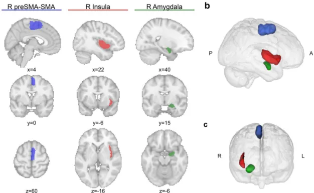
The right (R) preSMA and SMA, R insula, and R amyg-dala are prominently featured regions in CBP analyses, and were therefore selected as ROIs to evaluate our software (see Fig. 2). The R preSMA–SMA region (at 972 voxels) was extracted using the Juelich Cytoarchitectonic Atlas (Eickhoff et al. 2005; Ruan et al. 2018), and the R insula (546 voxels) and R amygdala (280 voxels) regions were both extracted using the FSL distributed Harvard-Oxford Atlas. The FIX-denoised rsfMRI data of 300 healthy unrelated subjects (mean age 28.57, 150 females, no significant age ( t = 0.71 ,
p = .48 ) and educational ( t = − 0.31 , p = .75 ) difference
between genders) from the HCP (Van Essen et al. 2013), and BEDPOSTX results of the minimally processed (Glasser et al. 2013) dMRI data of the same 300 subjects were used as input data for the rsfMRI and dMRI modalities, respectively.
Workflow execution proceeded separately for each ROI and modality, as depicted in Fig. 1. For each execution the average MNI152 T1 brain (2 mm isotropic) from FSL (Jen-kinson et al. 2012) was binarized and used as a whole-brain gray matter target mask. For rsfMRI only, the target mask was subsampled (see "ROI mask preprocessing") to improve computational efficiency.
Including the preprocessing of the ROI and target masks, all the following steps were done by CBPtools with the con-figuration parameters outlined below (these are the CBPtools default configuration parameters). The rsfMRI BOLD time series were 5 mm FWHM smoothed, global WM, global CSF, and 24 motion parameter signal corrected (including a bias term), and 0.01–0.08 Hz band-pass-filtered (see the green boxes in Fig. 1c). Global WM and global CSF nui-sance signal regression in addition to FIX-denoising was used as it appears to give the highest reliability for rsfMRI CBP (Plachti et al. 2019). The linear correlations between ROI and target voxel time series were then computed to obtain a ROI-to-target connectivity matrix for each subject
and Fisher’s Z transformed. To derive dMRI connectivity, probabilistic tractography was performed with the following parameters: distance threshold = 5, loop check = true, cur-vature threshold = 0.2, step length = 0.5, number of samples = 5000, steps per sample = 2000, correct path distribution for pathway length = true. This yielded a high-resolution ROI to low-resolution target (whole-brain) connectivity matrix per subject which was cubic transformed.
Each subject’s connectivity matrix was used as input for k-means clustering (with k from 2 to 5, the k-means++ initialization method, 256 initializations [as suggested by Nanetti et al. (2009), and a maximum of 10,000 iterations; Fig. 1d]. The range of k was chosen after consulting relevant literature regarding the three ROIs. To maintain the same settings for each ROI and make replication of the exam-ple procedure computationally less intensive, we chose to keep the range of k consistent between ROIs. To obtain a group-level clustering, hierarchical clustering with complete linkage and Hamming distance was applied (Fig. 1f) on individual-level clusterings to obtain a combined reference clustering per k (Nguyen and Caruana 2007). This reference clustering was subsequently used to relabel the individual clusterings. The resulting labels were used to calculate the
mode for each voxel, serving as the group-level clustering
result for each value of k. Cluster validation was performed
Fig. 2 Outline of the three ROIs used for the example procedure. a The three columns highlight the R preSMA–SMA (blue, left), R amygdala (green, middle), and R insula (red, right) in sagittal, coro-nal, and axial (top to bottom) sections. The figures were generated using Nilearn’s plotting tools (Abraham et al. 2014). b All ROIs
shown from a right-sided view with posterior (P) to the left, and ante-rior (A) to the right. c An anteante-rior view of the three ROIs, with right (R) and left (L) flipped to radiological display convention. The 3D representations in b and c were generated using Mango (multi-image analysis GUI; http://ric.uthsc sa.edu/mango /)
on the individual clusterings using the Silhouette index, the Calinski–Harabasz index, and the Davies–Bouldin index (Fig. 1e). The adjusted rand Index (ARI) was computed as a similarity measure between individual and group cluster-ings (Fig. 1g).
The results section is structured such that each ROI reflects a different aspect of the CBPtools workflow. For the preSMA–SMA ROI we highlighted the reproducibility of histological parcellations, for the insula we focussed on the subdivisions of various k cluster solutions for the group parcellations and, lastly, for the amygdala we evaluated the cluster validity metrics provided as output by the workflow. All output not highlighted here is available in the Online Resource.
Results
preSMA–SMA parcellation
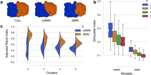
The group clusterings for the two-cluster solution approxi-mated the R preSMA–SMA cytoarchitectonic differen-tiation with an ARI of .71 for rsfMRI, and .76 for dMRI results (where 0 indicates no similarity at all, and 1 indi-cates perfect similarity). That is, only 76 (7.82%) and 63 (6.48%) out of all voxels were mismatched for rsfMRI and dMRI, respectively. Figure 3a provides a visual representa-tion of the ROI with the two-cluster labels mapped onto
it for the cytoarchitectonically defined region, and the two rCBP defined subdivisions using rsfMRI and dMRI data. The Silhouette index (Fig. 3c), Davies–Bouldin index, and Calinski–Harabasz index all indicated the two-cluster solution as the best fit to the rsfMRI input data (note that the Davies–Bouldin index indicates a better fit through a lower value). The Silhouette and Calinski–Harabasz indi-ces obtained from the dMRI clusterings both suggested the two-cluster solution, with only the Davies–Bouldin index suggesting a slightly better fit for the three-cluster solution. Our results are consistent with previous studies regarding functional and structural parcellation of the preSMA–SMA regions (Johansen-Berg et al. 2004; Klein et al. 2007; Kim et al. 2010; Zhang et al. 2015).
Insula parcellation
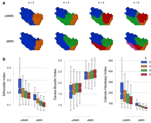
All internal validity metrics agreed that a two-cluster sepa-ration into an anterior and posterior subdivision fitted the rsfMRI source data best. The two- to five-cluster solu-tions are shown as 3D volumetric/voxel plots in Fig. 4. The three-cluster rsfMRI solution added a medial parcel (green), extending more into the anterior parcel (blue) rather than the posterior parcel (orange) of the two-cluster solution. The four-cluster rsfMRI solution further subdivided the medial and part of the posterior parcel into dorsal-anterior and medial parcels (green and red, respectively), whereas the five-cluster solution added only a thin parcel (magenta)
b
c
a
Fig. 3 R preSMA–SMA results from the rCBP procedure. a The two-cluster solutions of the combined R preSMA and SMA ROI for the cytoarchitectonically defined (Ruan et al. 2018) subdivision from the Jülich histological atlas (Eickhoff et al. 2005), and the rsfMRI and dMRI connectivity-based parcels from left to right. The 3D repre-sentations were generated using matplotlib’s 3D voxel/volumetric
plotting and are in the same view as Fig. 2b. b ARI scores between the individual subject clustering results and the group-level cluster-ing result for both rsfMRI and dMRI for k = [2, 3, 4, 5] . c Silhouette index for all cluster solutions ( k = [2, 3, 4, 5] ) where a higher Silhou-ette index indicates a bSilhou-etter fit. Here, the two-cluster solution seems to best fit the input data for both rsfMRI and dMRI
in between the aforementioned dorsal-anterior and medial parcels.
Likewise for dMRI data, the two-cluster solution sepa-rated the R insula into anterior and posterior subdivisions. However, the Davies–Bouldin index slightly diverged from the other metrics, instead suggesting a three-cluster solution to best fit the source data. The shape of the dMRI clusters also showed a different picture than the rsfMRI results, par-ticularly for the and five-cluster solutions. The three-cluster solution added a medial parcel that did not extend as much into the dorsal direction as the rsfMRI three-cluster solution did. Slightly more agreement between modalities was found in the four-cluster solution, where the posterior parcel was subdivided into a dorsal (blue) and ventral (red) part, the latter of which was further split into the five-cluster solution.
Functional parcellation of the two-cluster rsfMRI solution for the insula was in line with prior parcellations (Kelly et al.
2012). In addition, Nanetti et al. (2009) suggest a common
parcellation of the insula along the anterior-posterior axis for dMRI data. The four-cluster dMRI parcellation further-more visually resembles the insula’s functional differentia-tion uncovered by Kurth et al. (2010b) using a meta-analytic approach, with only our ventral-anterior parcel (red) extend-ing more anteriorly than theirs.
Amygdala parcellation
Similar to the other two ROIs, the model that best fits the data in the R amygdala was bipartite. Nevertheless, the two-cluster solutions for rsfMRI and dMRI connectivity dif-fered substantially (Fig. 5d, e). On the one hand, the rsfMRI two-cluster solution showed a dorsal (superior) and ventral (inferior) subdivision of the Amygdala. On the other hand, the dMRI two-cluster solution showed a medial and lateral subdivision. At higher clustering granularities clusters split further among the aforementioned axes, rather than finding common ground.
b
a
Fig. 4 R Insula results from the rCBP procedure. a Insula parcels for the two-, three-, four-, and five-cluster solutions obtained from rsfMRI (top row) and dMRI (bottom row) connectivity. All images are in the same view (right-sided) as Fig. 2b. b Internal validity
scores for all tested solutions ( k = [2, 3, 4, 5] ). The Silhouette index (left) and the Calinski–Harabasz index (right) indicate a better fit through a higher score, whereas the Davies–Bouldin index (middle) is better when lower
The Silhouette and Calinski–Harabasz indices (Fig. 5a) suggested a two-cluster solution to best fit the rsfMRI source data. However, the Davies–Bouldin index instead suggested a five-cluster solution to fit better. The two-cluster solution approximated prior functional parcellations of the amygdala (Mishra et al. 2014; Zhang et al. 2018) and also prior cyto-architectonic mapping of the region (Amunts et al. 2005). The dorsal cluster (orange) overlapped with the cytoarchi-tectonic outline of R amygdala centromedial and amygda-lostriatal subregions, whereas the ventral cluster (blue) over-lapped with the laterobasal and superficial subregions. At the three-cluster granularity, the ventral cluster was divided into a cluster resembling the cytoarchitectonic laterobasal
subregion (blue) and one resembling the superficial subre-gion (green), the latter of which is best seen from a left-sided view (Fig. S6b). The four-cluster solution subdivided mostly the dorsal cluster (orange), with the new cluster resembling the amygdalostriatal subregion. However, it appeared far larger than its cytoarchitectonic counterpart. The five-cluster solution further subdivided the ventral cluster (blue), but here no further cytoarchitectonic subdivisions exist.
For the dMRI clusterings, all validity indices (Fig. 5a) suggested a two-cluster solution to best fit the source data. As the clustering granularity increased, the R amygdala split further along its medial-lateral axis. Previous parcellation works using dMRI data (Solano-Castiella et al. 2010; Saygin
e
d
c
b
a
Fig. 5 Various CBPtools output figures for the R amygdala parcella-tion. a Internal validity scores for all tested solutions ( k = [2, 3, 4, 5] ). The Silhouette index (left) and the Calinski–Harabasz index (right) indicate a better fit through a higher score, whereas the Davies–Boul-din index (middle) is better when lower. b Group similarity scores
(i.e., the similarity of individual clusterings to the group clustering), with the cluster number k on the x-axis, comparing rsfMRI (blue) to dMRI (orange). c Relabel accuracy displayed in a similar format as b. d The two- and three-cluster solution of the R amygdala for rsfMRI. e the same for dMRI
et al. 2011; Fan et al. 2016; Wen et al. 2016) also found similar clusters along the medial-lateral axis. ARI similar-ity of individual clusterings to the group-level clustering (Fig. 5b) was higher for clusterings on dMRI data than on rsfMRI data, also reflected by the relabel accuracy (Fig. 5c).
Discussion
General pattern revealed by CBP
Separating the SMA and preSMA is a popular approach to validate rCBP methods (Johansen-Berg et al. 2004; Klein et al. 2007; Kim et al. 2010; Zhang et al. 2015), as it provides a gold standard and furthermore highlights the ability of the rCBP procedure to reproduce histological parcellations. These two neighboring regions exhibit an abrupt change in connectivity profile where their borders are expected to be, attributed to predominant connections to the motor regions for the SMA and prefrontal connections for the preSMA (Johansen-Berg et al. 2004). As voxels are assigned to clus-ters based on similarity in their connectivity profiles, sepa-rating the preSMA–SMA ROI through automated parcel-lation approaches should therefore be straightforward. By using the cytoarchitectonically defined preSMA and SMA regions as external validation, we were able to assess his-tological reproducibility of the preSMA–SMA ROI using
CBPtools. This was achieved with a very high similarity
(ARI > 0.7 ) for both the dMRI and the rsfMRI connectivity-driven parcellation to the cytoarchitectonic definition of the ROI.
While results for the preSMA–SMA parcellation were rather straightforward, this was not the case for the R insula parcellation for which many different suggestions for opti-mal cluster solutions exist in the literature (two-cluster (Cauda et al. 2011), three-cluster (Deen et al. 2011; Chang et al. 2013), and four-cluster (Kurth et al. 2010b), as well as various solutions exceeding our k-range (Kelly et al. 2012)). These differences may in part be caused by relatively small data sets with different properties, difficulties on account of intersubject alignment when delineating the ROI mask, as well as variability between research groups in their imple-mentation and use of methods and imaging modalities. Our results suggested a two-cluster solution to best fit both the dMRI and rsfMRI-based connectivity data, although this does not imply it is neurobiologically optimal. Early work on the insula has provided evidence for an anterior (dysgranu-lar) and posterior (granu(dysgranu-lar) subdivision separated by the central insular sulcus (Brodmann 1909). Cytoarchitectoni-cally the posterior insula can be further subdivided into two dorsal posterior areas and one ventral posterior area (Kurth et al. 2010a), but no evidence exists for the anterior insula. Whereas the two-cluster solution matched well between the
dMRI and rsfMRI modalities, the results diverged at the three- and five-cluster granularities. The mid-posterior clus-ter appearing in the dMRI four-clusclus-ter solution (Fig. 4a; red) and the mid-anterior cluster appearing in the rsfMRI four-cluster solution (red) made the solutions at the four-four-cluster granularity more similar. However, the rsfMRI mid-posterior cluster (green) extends more dorsally than its dMRI coun-terpart. Meta-analysis of the insula (Kurth et al. 2010b) resembles the four-cluster solution of the R insula, associ-ating the posterior cluster (blue) with sensorimotor function, the ventral-anterior cluster (orange) with social-emotional functions, the dorsal-anterior cluster (green) with cognitive functions, and the medial cluster (red) with chemical sensory functions. The medial cluster extends further into the pos-terior direction for the dMRI parcellations than is the case for the meta-analytic results, and in addition extends further dorsally for the rsfMRI parcellation.
For the R amygdala, the two-cluster solution best rep-resented the data for both the dMRI and rsfMRI modali-ties. The rsfMRI parcellation of the R amygdala that best fit the source data was a bipartite dorso-ventral subdivision. These results match earlier findings of Mishra et al. (2014), likewise a dorso-ventral (superior–inferior) subdivision in the two-cluster solution using functional connectivity, and a similar dorsal, ventral, and medial subdivision for the three-cluster solution. The same three-three-cluster solution was found by Zhang et al. (2018). Our validity metrics indicated a best fitting two-cluster solution, but as this does not necessarily imply neurobiological accuracy, a three-cluster solution is likewise viable. Furthermore, the parcellations visually cor-respond to the cytoarchitectonic mapping of the R amygdala (Amunts et al. 2005) up to the four-cluster solution.
Where a bipartite dorso-ventral subdivision of the amyg-dala best fits the rsfMRI data, the dMRI data instead best fits within a bipartite medio-lateral subdivision. This pattern resembles the two-cluster solution found by Solano-Castiella et al. (2010) and Fan et al. (2016) in that the solution divided the amygdala into a medial and a lateral cluster. Tract trac-ing of the rat amygdaloid complex shows that the medial amygdala is related to connections between both intrahemi-spheric amygdalae (Pikkarainen and Pitkänen 2001). The lateral amygdala is instead found to be connected to soma-tosensory cortical areas (Jolkkonen and Pitkänen 1998). Solano-Castiella et al. (2010) note the possible existence of a third cluster between the medial and lateral clusters, which resembles the pattern of clusters we found for the three-cluster solution.
The amygdala is a peculiar region on account of its spa-tial location, which may explain the differences between the rsfMRI and dMRI results. Whereas the rsfMRI parcellations resemble cytoarchictural subdivisions, the dMRI results may instead be driven by spatial artefacts on account of false positives in probabilistic fiber bundle tracking (Zalesky et al.
2016; Maier-Hein et al. 2017) of subcortical areas. As the region gets split at higher granularities, it is possible that instead of creating subdivisions on the basis of neurobiologi-cally relevant signals, instead the subdivisions are driven by noise in the signal on account of methodological idi-osyncracies. Investigating why such subdivisions occur at higher granularities is beyond the scope of this work, but is nonetheless an important consideration when investigating clusters with dMRI data. We further investigated whether parcellations of the R amygdala were driven by within-ROI and short-range connections. We parcellated dMRI data after excluding ROI-to-ROI connectivity (excluding 5 mm, 20 mm, and 40 mm border around the ROI in Online Resource Fig. S7), including a mapping of the linear correla-tions predominantly driving the parcellation results (Online Resource Fig. S9). The resulting parcellations remained mostly unchanged, exhibiting the same medio-lateral pat-tern of subdivisions.
Overall, divergence between validity indices (i.e., the Davies–Bouldin index from the other validity metrics) high-lights the importance of choosing a proper validity metric, each of which assesses cluster validity in a unique way. Note that comparisons of validity scores outside of the sample are meaningless, hence rsfMRI and dMRI validity scores can-not be directly compared. For the R insula the divergence is not necessarily surprising, as it shows transitional changes in cytoarchitecture (Kurth et al. 2010a), rather than sharp cytoarchitectonic borders present between the preSMA and SMA, making it difficult to define stable hard borders. Simi-larity of cluster labels between subject-wise clusterings may vary considerably. It is as of yet unclear what factors con-tribute to the high dissimilarity between subjects on some cluster solutions and for some ROIs. For instance, similarity values for the individual clustering results to the group-level clustering results on the two-cluster preSMA–SMA solution are high (see Online Resource Fig. S4b), which may imply that the regions have strongly divergent connectivity patterns that are stable between subjects. However, regions such as the amygdala show lower similarity values. This may in part be due to poor signal to noise ratio with MRI in the subcorti-cal regions (Noble et al. 2017). Nevertheless, the solutions showcased here can be found in previously published works. However, as far as we are aware, no data-driven cluster-ing was performed uscluster-ing dMRI data for the R amygdala at higher granularities.
Conclusions and perspectives
Here, we have demonstrated the effectiveness of using
CBPtools to procure resting-state functional and diffusion
MRI connectivity-derived parcellations on three function-ally and spatifunction-ally different ROIs. Connectivity and cluster-ing methods have been carefully chosen to both reflect the
most popular and the most widely evaluated approaches in the brain mapping community. The procedure is customiz-able through a configuration file, allowing for fine-tuned processing for each ROI. Furthermore, by providing or specifying input as well as parameters given to CBPtools, any parcellation work can be reproduced with relative ease and, importantly, can be compared to other works using this tool. To illustrate the efficiency of the procedure, we have provided benchmarks (see Online Resource Sect. 3.1 Benchmarks) as a guideline for what to expect when exe-cuting CBPtools on a similar data set, with similar set-tings, on an average computational cluster. Through the use of the CBPtools output, a user will be able to quickly generate parcellations and validity metrics that can either be used directly or used to inform a more detailed post hoc analysis. For instance, the selection of clustering granular-ity as well as multi-modal integration of cluster solutions may require further fine-grained and region-specific analy-ses. We opted to provide all k cluster solutions with guid-ance for the user to choose the optimal solution, as there likely is no ’one true parcellation’, but instead biologically relevant maps at different granularities.
Future development of the software will support the integration of MACM and structural covariance modali-ties, found to be valuable for studying the brain and adding an additional layer of information to multi-modal CBP (Eickhoff et al. 2015; Plachti et al. 2019). In the framework of the Human Brain Project and in collaboration with the Juelich Supercomputing Center, a web-based version of the software that can execute the rCBP procedure on vari-ous predefined and preprocessed large data sets is planned. This will offer a high-throughput solution for massive par-allelization for rCBP on a user-defined ROI, in an online environment where all summary output will be available for download.
In summary, we provide an openly distributed package for performing rCBP for which to our knowledge there is currently no alternative. We have outlined its procedure and demonstrated its efficacy using three commonly par-cellated ROIs on a substantial data set. By introducing
CBPtools we provide researchers the means to conduct
reproducible, data-driven rCBP analyses on multiple neu-roimaging modalities and large amounts of subject data.
Acknowledgements Open Access funding provided by Projekt DEAL. Our thanks go to Kyesam Jung and Jianxiao Wu for testing CBPtools and providing useful feedback, as well as Benjamin Poldrack and Alex Waite for help in making the example data available.
Funding This study was supported by the European Union’s Horizon 2020 Research and Innovation Programme under Grant Agreement no. 785907 (HBP SGA2) and Grant Agreement no. 7202070 (HBP SGA1). SG is supported by the Deutsche Forschungsgemeinschaft (DFG) under Grant Agreement GE 2835/1-1.
Compliance with ethical standards
Conflict of interest The authors declare that they have no conflict of interest.
Ethical approval The Institutional Review Board at the Washington University in St. Louis approved the HCP study. Informed consent was obtained from all individual participants included in the study. All procedures performed in this study were in accordance with the ethical standards of the institutional research committee (Ethikkommission der Med. Fakultät der HHU Düsseldorf, project number 4039). This article does not contain any studies with animals performed by any of the authors.
Informed consent Informed consent was obtained from all individual participants included in the study by the Human Connectome Project consortium.
Open Access This article is licensed under a Creative Commons Attri-bution 4.0 International License, which permits use, sharing, adapta-tion, distribution and reproduction in any medium or format, as long as you give appropriate credit to the original author(s) and the source, provide a link to the Creative Commons licence, and indicate if changes were made. The images or other third party material in this article are included in the article’s Creative Commons licence, unless indicated otherwise in a credit line to the material. If material is not included in the article’s Creative Commons licence and your intended use is not permitted by statutory regulation or exceeds the permitted use, you will need to obtain permission directly from the copyright holder. To view a copy of this licence, visit http://creat iveco mmons .org/licen ses/by/4.0/.
References
Abraham A, Pedregosa F, Eickenberg M, Gervais P, Mueller A, Kos-saifi J, Gramfort A, Thirion B, Varoquaux G (2014) Machine learning for neuroimaging with scikit-learn. Front Neuroinfor-matics 8:14. https ://doi.org/10.3389/fninf .2014.00014
Amunts K, Kedo O, Kindler M, Pieperhoff P, Mohlberg H, Shah NJ, Habel U, Schneider F, Zilles K (2005) Cytoarchitectonic mapping of the human amygdala, hippocampal region and entorhinal cor-tex: intersubject variability and probability maps. Anat Embryol 210(5–6):343–352. https ://doi.org/10.1007/s0042 9-005-0025-5 Baarsch J, Celebi ME (2012) Investigation of internal validity
meas-ures for k-means clustering. Proc Int MultiConf Eng Comput Sci I:14–16
Bajada CJ, Jackson RL, Haroon HA, Azadbakht H, Parker GJM, Lam-bon Ralph MA, Cloutman LL (2017) A graded tractographic parcellation of the temporal lobe. Neuroimage. https ://doi. org/10.1016/j.neuro image .2017.04.016
Barron DS, Eickhoff SB, Clos M, Fox PT (2015) Human pulvinar functional organization and connectivity. Hum Brain Mapp 36(7):2417–2431. https ://doi.org/10.1002/hbm.22781
Behrens TEJ, Johansen-Berg H, Woolrich MW, Smith SM, Wheeler-Kingshott CAM, Boulby PA, Barker GJ, Sillery EL, Sheehan K, Ciccarelli O et al (2003) Non-invasive mapping of connections between human thalamus and cortex using diffusion imaging. Nat Neurosci 6(7):750–757. https ://doi.org/10.1038/nn107 5 Brett M, Markiewicz CJ, Hanke M, Côté MA, Cipollini B, McCarthy
P, Cheng CP, Halchenko YO, Cottaar M, Ghosh S, Larson E, Was-sermann D, Gerhard S, Lee GR, Kastman E, Rokem A, Madison C, Morency FC, Moloney B, Burns C, Millman J, Gramfort A,
Leppäkangas J, Markello R, van den Bosch JJ, Vincent RD, Sub-ramaniam K, Raamana PR, Nichols BN, Baker EM, Goncalves M, Hayashi S, Pinsard B, Haselgrove C, Hymers M, Koudoro S, Oosterhof NN, Amirbekian B, Nimmo-Smith I, Nguyen L, Red-digari S, St-Jean S, Garyfallidis E, Varoquaux G, Kaczmarzyk J, Legarreta JH, Hahn KS, Hinds OP, Fauber B, Poline JB, Stutters J, Jordan K, Cieslak M, Moreno ME, Haenel V, Schwartz Y, Thirion B, Papadopoulos Orfanos D, Pérez-García F, Solovey I, Gonzalez I, Lecher J, Leinweber K, Raktivan K, Fischer P, Gervais P, Gadde S, Ballinger T, Roos T, Reddam VR, Freec84 (2019) nipy/nibabel: 2.4.0. Zenodo. https ://doi.org/10.5281/zenod o.26206 14, https :// zenod o.org/recor d/26206 14. Accessed 11 May 2019
Brodmann K (1909) Vergleichende lokalisationslehre der grosshirn-rinde. Johann Ambrosius Barth, Leipzig
Bzdok D, Laird AR, Zilles K, Fox PT, Eickhoff SB (2013) An investi-gation of the structural, connectional, and functional subspeciali-zation in the human amygdala. Hum Brain Mapp 34(12):3247– 3266. https ://doi.org/10.1002/hbm.22138
Bzdok D, Heeger A, Langner R, Laird AR, Fox PT, Palomero-Gal-lagher N, Vogt BA, Zilles K, Eickhoff SB (2015) Subspecializa-tion in the human posterior medial cortex. Neuroimage 106:55– 71. https ://doi.org/10.1016/j.neuro image .2014.11.009
Calinski T, Harabasz J (1974) A dendrite method for cluster analy-sis. Commun Stat Theory Methods 3(1):1–27. https ://doi. org/10.1080/03610 92740 88271 01
Caspers S, Moebus S, Lux S, Pundt N, Schütz H, Mühleisen TW, Gras V, Eickhoff SB, Romanzetti S, Stöcker T, Stirnberg R, Kirlangic ME, Minnerop M, Pieperhoff P, Mödder U, Das S, Evans AC, Jöckel KH, Erbel R, Cichon S, Nöthen MM, Sturma D, Bauer A, Jon Shah N, Zilles K, Amunts K (2014) Studying variability in human brain aging in a population-based german cohort-rationale and design of 1000BRAINS. Front Aging Neurosci 6:149. https ://doi.org/10.3389/fnagi .2014.00149
Cauda F, D’Agata F, Sacco K, Duca S, Geminiani G, Vercelli A (2011) Functional connectivity of the insula in the resting brain. Neuroimage 55(1):8–23. https ://doi.org/10.1016/j.neuro image .2010.11.049
Chang LJ, Yarkoni T, Khaw MW, Sanfey AG (2013) Decoding the role of the insula in human cognition: functional parcellation and large-scale reverse inference. Cereb Cortex 23(3):739–749. https ://doi.org/10.1093/cerco r/bhs06 5
Chase HW, Clos M, Dibble S, Fox P, Grace AA, Phillips ML, Eickhoff SB (2015) Evidence for an anterior-posterior differentiation in the human hippocampal formation revealed by meta-analytic parcella-tion of fMRI coordinate maps: focus on the subiculum. Neuroim-age 113:44–60. https ://doi.org/10.1016/j.neuro imNeuroim-age .2015.02.069 Clos M, Amunts K, Laird AR, Fox PT, Eickhoff SB (2013) Tackling
the multifunctional nature of Broca’s region meta-analytically: co-activation-based parcellation of area 44. Neuroimage 83:174–188. https ://doi.org/10.1016/j.neuro image .2013.06.041
Cohen AL, Fair DA, Dosenbach NUF, Miezin FM, Dierker D, Van Essen DC, Schlaggar BL, Petersen SE (2008) Defining functional areas in individual human brains using resting functional connec-tivity MRI. Neuroimage 41(1):45–57. https ://doi.org/10.1016/j. neuro image .2008.01.066
Cramér H (1946) Mathematical methods of statistics, reprint edn. Princeton University Press, Princeton
Davies DL, Bouldin DW (1979) A cluster separation measure. IEEE Trans Pattern Anal Mach Intell 1(2):224–227. https ://doi. org/10.1109/TPAMI .1979.47669 09
Deen B, Pitskel NB, Pelphrey KA (2011) Three systems of insular functional connectivity identified with cluster analysis. Cereb Cortex 21(7):1498–1506. https ://doi.org/10.1093/cerco r/bhq18 6 Eickhoff SB, Stephan KE, Mohlberg H, Grefkes C, Fink GR,
probabilistic cytoarchitectonic maps and functional imaging data. Neuroimage 25(4):1325–1335. https ://doi.org/10.1016/j.neuro image .2004.12.034
Eickhoff SB, Thirion B, Varoquaux G, Bzdok D (2015) Connectivity-based parcellation: critique and implications. Hum Brain Mapp 36(12):4771–4792. https ://doi.org/10.1002/hbm.22933
Eickhoff SB, Laird AR, Fox PT, Bzdok D, Hensel L (2016) Functional segregation of the human dorsomedial prefrontal cortex. Cereb Cortex 26(1):304–321. https ://doi.org/10.1093/cerco r/bhu25 0 Eickhoff SB, Yeo BTT, Genon S (2018) Imaging-based parcellations
of the human brain. Nat Rev Neurosci 19(11):672–686. https :// doi.org/10.1038/s4158 3-018-0071-7
Fan L, Li H, Zhuo J, Zhang Y, Wang J, Chen L, Yang Z, Chu C, Xie S, Laird AR, Fox PT, Eickhoff SB, Yu C, Jiang T (2016) The human brainnetome atlas: a new brain atlas based on connec-tional architecture. Cereb Cortex 26(8):3508–3526. https ://doi. org/10.1093/cerco r/bhw15 7
Genon S, Li H, Fan L, Müller VI, Cieslik EC, Hoffstaedter F, Reid AT, Langner R, Grefkes C, Fox PT et al (2017) The right dor-sal premotor mosaic: organization, functions, and connectivity. Cerebral Cortex 27(3):2095–2110. https ://doi.org/10.1093/cerco r/bhw06 5
Genon S, Reid A, Li H, Fan L, Müller VI, Cieslik EC, Hoffstaedter F, Langner R, Grefkes C, Laird AR, Fox PT, Jiang T, Amunts K, Eickhoff SB (2018) The heterogeneity of the left dorsal premotor cortex evidenced by multimodal connectivity-based parcellation and functional characterization. Neuroimage 170:400–411. https ://doi.org/10.1016/j.neuro image .2017.02.034
Glasser MF, Sotiropoulos SN, Wilson JA, Coalson TS, Fischl B, Andersson JL, Xu J, Jbabdi S, Webster M, Polimeni JR, Van Essen DC, Jenkinson M, Consortium WMH (2013) The mini-mal preprocessing pipelines for the Human Connectome Project. Neuroimage 80:105–124. https ://doi.org/10.1016/j.neuro image .2013.04.127
Hardwick RM, Lesage E, Eickhoff CR, Clos M, Fox P, Eickhoff SB (2015) Multimodal connectivity of motor learning-related dor-sal premotor cortex. Neuroimage 123:114–128. https ://doi. org/10.1016/j.neuro image .2015.08.024
Hastie T, Tibshirani R, Friedman J (2013) The elements of statistical learning: data mining, inference, and prediction, illustrated edn. Springer Science & Business Media, New York
Hubert L, Arabie P (1985) Comparing partitions. J Classif 2(1):193– 218. https ://doi.org/10.1007/BF019 08075
Hutchison RM, Womelsdorf T, Allen EA, Bandettini PA, Calhoun VD, Corbetta M, Della Penna S, Duyn JH, Glover GH, Gonzalez-Cas-tillo J, Handwerker DA, Keilholz S, Kiviniemi V, Leopold DA, de Pasquale F, Sporns O, Walter M, Chang C (2013) Dynamic functional connectivity: promise, issues, and interpretations. Neuroimage 80:360–378. https ://doi.org/10.1016/j.neuro image .2013.05.079
Jenkinson M, Beckmann CF, Behrens TEJ, Woolrich MW, Smith SM (2012) FSL. Neuroimage 62(2):782–790. https ://doi. org/10.1016/j.neuro image .2011.09.015
Ji B, Li Z, Li K, Li L, Langley J, Shen H, Nie S, Zhang R, Hu X (2016) Dynamic thalamus parcellation from resting-state fMRI data. Hum Brain Mapp 37(3):954–967. https ://doi.org/10.1002/ hbm.23079
Johansen-Berg H, Behrens TEJ, Robson MD, Drobnjak I, Rushworth MFS, Brady JM, Smith SM, Higham DJ, Matthews PM (2004) Changes in connectivity profiles define functionally distinct regions in human medial frontal cortex. Proc Natl Acad Sci USA 101(36):13335–13340. https ://doi.org/10.1073/pnas.04037 43101 Jolkkonen E, Pitkänen A (1998) Intrinsic connections of the rat amyg-daloid complex: projections originating in the central nucleus. J Comp Neurol 395(1):53–72. https ://doi.org/10.1002/(sici)1096-9861(19980 525)395:1%3C53::aid-cne5%3E3.0.co;2-g
Jones E, Oliphant T, Peterson P (2001) SciPy: open source scientific tools for Python. https ://www.scipy .org/. Accessed 18 Dec 2019 Kelly C, Toro R, Di Martino A, Cox CL, Bellec P, Castellanos FX,
Mil-ham MP (2012) A convergent functional architecture of the insula emerges across imaging modalities. Neuroimage 61(4):1129– 1142. https ://doi.org/10.1016/j.neuro image .2012.03.021 Kim JH, Lee JM, Jo HJ, Kim SH, Lee JH, Kim ST, Seo SW, Cox
RW, Na DL, Kim SI, Saad ZS (2010) Defining functional SMA and pre-SMA subregions in human MFC using resting state fMRI: functional connectivity-based parcellation method. Neu-roimage 49(3):2375–2386. https ://doi.org/10.1016/j.neuro image .2009.10.016
Klein JC, Behrens TEJ, Robson MD, Mackay CE, Higham DJ, Johansen-Berg H (2007) Connectivity-based parcellation of human cortex using diffusion MRI: establishing reproducibility, validity and observer independence in BA 44/45 and SMA/pre-SMA. Neuroimage 34(1):204–211. https ://doi.org/10.1016/j.neuro image .2006.08.022
Köster J, Rahmann S (2012) Snakemake-a scalable bioinformatics workflow engine. Bioinformatics 28(19):2520–2522. https ://doi. org/10.1093/bioin forma tics/bts48 0
Kurth F, Eickhoff SB, Schleicher A, Hoemke L, Zilles K, Amunts K (2010a) Cytoarchitecture and probabilistic maps of the human posterior insular cortex. Cereb Cortex 20(6):1448–1461. https :// doi.org/10.1093/cerco r/bhp20 8
Kurth F, Zilles K, Fox PT, Laird AR, Eickhoff SB (2010b) A link between the systems: functional differentiation and integra-tion within the human insula revealed by meta-analysis. Brain Struct Funct 214(5–6):519–534. https ://doi.org/10.1007/s0042 9-010-0255-z
Maier-Hein KH, Neher PF, Houde JC, Côté MA, Garyfallidis E, Zhong J, Chamberland M, Yeh FC, Lin YC, Ji Q, Reddick WE, Glass JO, Chen DQ, Feng Y, Gao C, Wu Y, Ma J, He R, Li Q, Wes-tin CF, Deslauriers-Gauthier S, González JOO, Paquette M, St-Jean S, Girard G, Rheault F, Sidhu J, Tax CMW, Guo F, Mesri HY, Dávid S, Froeling M, Heemskerk AM, Leemans A, Boré A, Pinsard B, Bedetti C, Desrosiers M, Brambati S, Doyon J, Sarica A, Vasta R, Cerasa A, Quattrone A, Yeatman J, Khan AR, Hodges W, Alexander S, Romascano D, Barakovic M, Auría A, Esteban O, Lemkaddem A, Thiran JP, Cetingul HE, Odry BL, Mailhe B, Nadar MS, Pizzagalli F, Prasad G, Villalon-Reina JE, Galvis J, Thompson PM, Requejo FS, Laguna PL, Lacerda LM, Barrett R, Dell’Acqua F, Catani M, Petit L, Caruyer E, Daducci A, Dyrby TB, Holland-Letz T, Hilgetag CC, Stieltjes B, Desco-teaux M (2017) The challenge of mapping the human connectome based on diffusion tractography. Nat Commun 8:1349. https ://doi. org/10.1038/s4146 7-017-01285 -x
Maulik U, Bandyopadhyay S (2002) Performance evaluation of some clustering algorithms and validity indices. IEEE Trans Pattern Anal Mach Intell 24(12):1650–1654. https ://doi.org/10.1109/ TPAMI .2002.11148 56
Mishra A, Rogers BP, Chen LM, Gore JC (2014) Functional connectiv-ity-based parcellation of amygdala using self-organized mapping: a data driven approach. Hum Brain Mapp 35(4):1247–1260. https ://doi.org/10.1002/hbm.22249
Muhle-Karbe PS, Derrfuss J, Lynn MT, Neubert FX, Fox PT, Brass M, Eickhoff SB (2016) Co-activation-based parcellation of the lateral prefrontal cortex delineates the inferior frontal junction area. Cereb Cortex 26(5):2225–2241. https ://doi.org/10.1093/ cerco r/bhv07 3
Nanetti L, Cerliani L, Gazzola V, Renken R, Keysers C (2009) Group analyses of connectivity-based cortical parcellation using repeated k-means clustering. Neuroimage 47(4):1666–1677. https ://doi. org/10.1016/j.neuro image .2009.06.014
Nguyen N, Caruana R (2007) Consensus clusterings. In: Seventh IEEE international conference on data mining (ICDM 2007), pp 607– 612. https ://doi.org/10.1109/ICDM.2007.73
Noble S, Spann MN, Tokoglu F, Shen X, Constable RT, Scheinost D (2017) Influences on the test-retest reliability of functional con-nectivity MRI and its relationship with behavioral utility. Cereb Cortex 27(11):5415–5429. https ://doi.org/10.1093/cerco r/bhx23 0 Oliphant T (2006) A guide to NumPy. Trelgol Publishing, Spanish
Fork. https ://www.resea rchga te.net/publi catio n/21387 7900_Guide _to_NumPy . Accessed 27 Mar 2019
Pedregosa F, Varoquaux G, Gramfort A, Michel V, Thirion B, Grisel O, Blondel M, Prettenhofer P, Weiss R, Dubourg V, Vanderplas J, Passos A, Cournapeau D, Brucher M, Perrot M, Duchesnay É (2011) Scikit-learn: machine learning in Python. J Mach Learn Res 12:2825–2830
Pikkarainen M, Pitkänen A (2001) Projections from the lateral, basal and accessory basal nuclei of the amygdala to the perirhinal and postrhinal cortices in rat. Cereb Cortex 11(11):1064–1082. https ://doi.org/10.1093/cerco r/11.11.1064
Plachti A, Eickhoff SB, Hoffstaedter F, Patil KR, Laird AR, Fox PT, Amunts K, Genon S (2019) Multimodal parcellations and exten-sive behavioral profiling tackling the hippocampus gradient. Cereb Cortex. https ://doi.org/10.1093/cerco r/bhy33 6
Pruim RHR, Mennes M, van Rooij D, Llera A, Buitelaar JK, Beckmann CF (2015) ICA-AROMA: a robust ICA-based strategy for remov-ing motion artifacts from fMRI data. Neuroimage 112:267–277. https ://doi.org/10.1016/j.neuro image .2015.02.064
Rand WM (1971) Objective criteria for the evaluation of cluster-ing methods. J Am Stat Assoc 66(336):846–850. https ://doi. org/10.1080/01621 459.1971.10482 356
Reuter N (2019) CBPtools documentation. https ://cbpto ols.readt hedoc s.io/en/lates t/. Accessed 18 Dec 2019
Rousseeuw PJ (1987) Silhouettes: a graphical aid to the interpretation and validation of cluster analysis. J Comput Appl Math 20:53–65. https ://doi.org/10.1016/0377-0427(87)90125 -7
Ruan J, Bludau S, Palomero-Gallagher N, Caspers S, Mohlberg H, Eickhoff SB, Seitz RJ, Amunts K (2018) Cytoarchitecture, prob-ability maps, and functions of the human supplementary and pre-supplementary motor areas. Brain Struct Funct 223(9):4169– 4186. https ://doi.org/10.1007/s0042 9-018-1738-6
Salimi-Khorshidi G, Douaud G, Beckmann CF, Glasser MF, Griffanti L, Smith SM (2014) Automatic denoising of functional MRI data: combining independent component analysis and hierarchi-cal fusion of classifiers. Neuroimage 90:449–468. https ://doi. org/10.1016/j.neuro image .2013.11.046
Saygin ZM, Osher DE, Augustinack J, Fischl B, Gabrieli JDE (2011) Connectivity-based segmentation of human amygdala nuclei using probabilistic tractography. Neuroimage 56(3):1353–1361. https :// doi.org/10.1016/j.neuro image .2011.03.006
Schaefer A, Kong R, Gordon EM, Laumann TO, Zuo XN, Holmes AJ, Eickhoff SB, Yeo BTT (2018) Local-global parcellation of the human cerebral cortex from intrinsic functional connectivity MRI. Cereb Cortex 28(9):3095–3114. https ://doi.org/10.1093/ cerco r/bhx17 9
Solano-Castiella E, Anwander A, Lohmann G, Weiss M, Docherty C, Geyer S, Reimer E, Friederici AD, Turner R (2010) Diffusion tensor imaging segments the human amygdala in vivo. Neuro-image 49(4):2958–2965. https ://doi.org/10.1016/j.neuro Neuro-image .2009.11.027
Van Essen DC, Smith SM, Barch DM, Behrens TEJ, Yacoub E, Ugur-bil K, Consortium WMH (2013) The WU-Minn Human Con-nectome Project: an overview. Neuroimage 80:62–79. https ://doi. org/10.1016/j.neuro image .2013.05.041
Vinh NX, Epps J, Bailey J (2010) Information theoretic measures for clusterings comparison: Variants, properties, normalization and correction for chance. J Mach Learn Res 11:2837–2854 Von Luxburg U (2007) A tutorial on spectral clustering. Stat Comput
17(4):395–416. https ://doi.org/10.1007/s1122 2-007-9033-z Wang J, Yang Y, Fan L, Xu J, Li C, Liu Y, Fox PT, Eickhoff SB,
Yu C, Jiang T (2015) Convergent functional architecture of the superior parietal lobule unraveled with multimodal neuroimag-ing approaches. Hum Brain Mapp 36(1):238–257. https ://doi. org/10.1002/hbm.22626
Wen Q, Stirling BD, Sha L, Shen L, Whalen PJ, Wu YC (2016) Parcel-lation of human amygdala subfields using orientation distribution function and spectral k-means clustering. Comput Diffus MRI 2016:123–132. https ://doi.org/10.1007/978-3-319-54130 -3_10 Zalesky A, Fornito A, Cocchi L, Gollo LL, van den Heuvel MP,
Breakspear M (2016) Connectome sensitivity or specificity: which is more important? Neuroimage 142:407–420. https ://doi. org/10.1016/j.neuro image .2016.06.035
Zhang Y, Caspers S, Fan L, Fan Y, Song M, Liu C, Mo Y, Roski C, Eickhoff S, Amunts K, Jiang T (2015) Robust brain parcel-lation using sparse representation on resting-state fMRI. Brain Struct Funct 220(6):3565–3579. https ://doi.org/10.1007/s0042 9-014-0874-x
Zhang X, Cheng H, Zuo Z, Zhou K, Cong F, Wang B, Zhuo Y, Chen L, Xue R, Fan Y (2018) Individualized functional parcellation of the human amygdala using a semi-supervised clustering method: a 7 T resting state fMRI study. Front Neurosci 12:270. https ://doi. org/10.3389/fnins .2018.00270
Publisher’s Note Springer Nature remains neutral with regard to jurisdictional claims in published maps and institutional affiliations
![Fig. 5 Various CBPtools output figures for the R amygdala parcella- parcella-tion. a Internal validity scores for all tested solutions ( k = [2, 3, 4, 5] )](https://thumb-eu.123doks.com/thumbv2/123doknet/6106586.155166/10.892.127.775.87.704/various-cbptools-amygdala-parcella-parcella-internal-validity-solutions.webp)
