1
SEMANTIC ANNOTATION OF GPS TRACES: ACTIVITY TYPE INFERENCE 2
3
Sofie Reumers1*, Feng Liu1, Davy Janssens1, Mario Cools2,1,3, and Geert Wets1 4
5
1 Transportation Research Institute (IMOB), Hasselt University 6
Wetenschapspark 5, bus 6, BE-3590 Diepenbeek, Belgium 7
Fax.: +32(0)11 26 91 99 8
9
2 Transport, Logistique, Urbanisme et Conception (TLU+C), Université de Liège 10
Chemin des Chevreuils 1, Bât. 52/3, BE-4000 Liège, Belgium 11
12
3 Centre for Information, Modeling and Simulation (CIMS), Hogeschool-Universiteit Brussel 13
Warmoesberg 26, BE-1000 Brussels, Belgium 14 15 16 Sofie Reumers 17 Tel.: +32(0)11 26 91 60 18 Email: [email protected] 19 20 Feng Liu 21 Tel.: +32(0)11 26 91 25 22 Email: [email protected] 23 24 Davy Janssens 25 Tel.: +32(0)11 26 91 28 26 Email: [email protected] 27 28 Mario Cools 29 Tel.: +32(0)485 42 71 55 30 Email: [email protected] 31 32 Geert Wets 33 Tel.: +32(0)11 26 91 58 34 Email: [email protected] 35 36 37 38 * Corresponding author 39 40 41 Number of words = 4997 42
Number of tables and figures = 7 43
Words count: 4997 + 7*250 = 6747 words 44
45
Paper submitted: November 14, 2012 46
ABSTRACT 47
48
Due to the rapid development of technology, larger data sets concerning activity travel behavior become 49
available. These data sets often lack semantic interpretation. This implies that annotation in terms of activity 50
type and transportation mode is necessary. This paper aims to infer activity types from GPS traces by developing 51
a decision tree-based model. The model only considers activity start times and activity durations. Based on the 52
decision tree classification, a probability distribution and a point prediction model were constructed. The 53
probability matrix describes the probability of each activity type for each class (i.e. combination of activity start 54
time and activity duration). In each class, the point prediction model selects the activity type that has the highest 55
probability. Two types of data were collected in 2006 and 2007 in Flanders, Belgium, i.e. activity travel data and 56
GPS data. The optimal classification tree constructed comprises 18 leaves. Consequently, 18 if-then rules were 57
derived. An accuracy of 74% was achieved when training the tree. The accuracy of the model for the validation 58
set, i.e. 72.5%, shows that overfitting is minimal. When applying the model to the test set, the accuracy was 59
almost 76%. The models indicate the importance of time information in the semantic enrichment process. This 60
study contributes to future data collection in that it enables researchers to directly infer activity types from 61
activity start time and duration information obtained from GPS data. Because no location information is needed, 62
this research can be easily and readily implemented to millions of individual agents. 63
1 INTRODUCTION 64
65
The current research challenges in travel behavior analysis and travel demand modeling, such as obtaining more 66
detailed information and a better behavioral reflection of peoples’ choices, often reflect data problems (1). 67
Although widely used as data collection methodologies in travel behavior research, travel surveys and activity 68
diaries impose a significant respondent burden. Such surveys are very expensive and some survey methods, e.g. 69
the paper-and-pencil diary, impose a time lag between the data collection process and the data entry. Moreover, 70
the spatial and temporal components of the data collected are subject to biases. Also, traditional travel behavior 71
surveys often incur low response rates. These shortcomings have been well reported in the literature, e.g. (1-6). 72
GPS data collection tools are a possible solution to these problems. A full-fledged activity based model 73
system fully reflects spatial and temporal constraints and opportunities, models interactions among agents, 74
captures time use and allocation behavior, and considers (both in-home and out-of-home) activity participation 75
along the continuous time dimension (7). GPS-based data collection tools, especially when combined with 76
activity-travel survey efforts, largely contributed to this by offering rich and detailed data about aspects of 77
behavior (7). GPS data provides accurate spatial as well as temporal data on travel patterns, i.e. the exact 78
coordinates and timestamps. The temporal component of diary data, on the other hand, is subject to rounding 79
issues, while there is often no or only limited spatial information collected in a diary survey. Therefore, GPS-80
based data collection experiments are, nowadays, often combined with activity-travel diary surveys to 81
supplement the information obtained from diary surveys as to obtain richer and more detailed data about travel 82
behavior and the underlying decision processes (8). 83
However, obtaining significant mobility knowledge from raw data of individual trajectories requires 84
detailed processing analysis. Large amounts of data are required to develop the most advanced activity-based 85
models that are sensitive to a multitude of travel demand management strategies. Due to the rapid development 86
of technology, an extensive growth in travel and activity behavior data exists to date while continuously 87
expanding. These technologies offer a solution to the challenges associated with conventional travel surveys. 88
The results are massive amounts of big data sets. However, despite the elimination of the above mentioned data 89
challenges, large data sets lack semantic interpretation, and should thus be augmented to increase its usefulness 90
in supporting the decisions of mobility management. As such, only detailed spatial and temporal resolutions are 91
covered by GPS, which means that an annotation of the activity being pursued or the transportation mode being 92
used is still necessary, explaining why current GPS-based data collection experiments are combined with 93
traditional paper surveys. 94
In this paper, a semantic annotation of GPS traces will be discussed. This annotation is mainly based on 95
heuristics (i.e. if-then rules) that are derived from the activity time information of an activity-travel diary survey 96
(9), and are applied to the GPS traces of an associated GPS survey to infer activity type information. The 97
information from the diary survey is used for model calibration and estimation. The data from the associated 98
GPS survey is used to test the model and to assure the method is applicable when only GPS data is available. 99
The resulting heuristics could mean an important improvement for the travel and activity behavior data 100
collection process and the problems associated with it, since data collection by means of GPS-devices or mobile 101
phone no longer need to be associated with a supplementary diary survey to annotate the activities. When fully 102
annotated, travel diaries can be reconstructed (i.e. estimation of the complete activity-travel schedule of 103
respondents) from GPS traces and can be fed into activity-based models. Therefore, the main purpose of this 104
research is the development of an expert system that links GPS trajectories to the corresponding activity type, by 105
merging the raw and behaviorally poor big data with the smaller but behaviorally richer travel survey data using 106
machine learning algorithms. Two models, i.e. a predicted probability distribution and a point prediction model, 107
were derived from a decision tree classification. The inference of activity information, solely from GPS data, 108
reduces the large data collection efforts associated with conventional diary surveys and even eliminates the use 109
of paper diary surveys for certain research purposes. The heuristics resulting from this research can be applied to 110
large data sets, in which only activity time information is available. 111
In literature, many studies (e.g. (10-15)) can be found in which the relationship between the activity, its 112
start time and its duration is analyzed. In most of these studies, additional information (e.g. land use data) was 113
used as well. In the procedure used by Stopher et al. (16), land use data is even the most important data source 114
for deducing the trip purpose (and transportation mode) from GPS traces. McGowen (17) also investigated the 115
use of GPS devices in replacing diary surveys. The models predicted in which of 26 different activity types the 116
individual participated. The best model, predicting out-of-home activities, was 63% accurate, while increasing 117
up to 79% when combined with home activities. Even though McGowen uses several methods for model 118
development, he explains that only classification trees are able to show the structure of the model and, in this 119
way, offer an additional validation method (i.e. by determining if the splits of the tree seem logical). However, 120
in his doctoral dissertation, McGowen does not provide simple heuristics (i.e. if-then rules) that can be extracted 121
from the classification tree constructed. Despite the more than modest contribution on the semantic annotation of 122
GPS traces in the literature, more specifically regarding the activity purpose, to the authors’ knowledge none of 123
these studies explicitly offer heuristics that can be applied in future research efforts. This research attempts to 124
meet that shortfall by listing the resulting if-then rules. 125
Furthermore, many studies also address the inference of transportation modes from raw GPS data (e.g. 126
(16), (18), (19), (20)). Even in this respect, explicit inference heuristics are rarely presented in the literature, for 127
example in (19). The approach presented is oriented towards an inference from raw GPS data without additional 128
information. Even here, the authors point out that detailed land use data will be necessary when extending their 129
approach to determine activity purposes. 130
In the field of data mining and informatics, a number of prominent machine learning algorithms exist 131
and are being used in modern computing applications. A common application for these algorithms often 132
involves decision-based classification and adaptive learning over a training set. As explained by Drazin and 133
Montag (21), a decision tree is a decision-modeling tool that graphically displays the classification process of a 134
given input for given output class labels. 135
The remainder of the paper is structured as follows. Section 2 describes the data, with respect to data 136
collection, data processing, some descriptive statistics of the data and potential errors in the data used for 137
analysis. In section 3, the research methodology is clarified. Finally, in the last section, the most important 138
results are discussed. This section also elaborates on some potential future research ideas. 139
140 141
2 DATA 142
2.1 Data Collection and Data Description 143
144
The data used for this study stems from a mixed-mode survey design, in which two types of data collection 145
methods were used, namely a paper-and-pencil activity-travel diary survey and a corresponding survey in which 146
GPS-enabled PDA’s (Personal Digital Assistants) were used. The data were collected in 2006 and 2007 in 147
Flanders, Belgium, in the context of a large scale survey that was conducted on 2500 households in the study 148
area. A more thorough elaboration on this survey can be found in (9). 149
In the paper-and pencil diary survey, the respondents recorded trip (and activity type) information 150
during the course of one week, such as the transportation mode, the travel party, information on the activity, and 151
so on. The trip time information, i.e. the trip start time and the trip end time, is also recorded. However, since the 152
diary is often filled out at the end of a survey day, this is merely an approximation for which the proximity is 153
determined by the recall skills of the respondent. Half of the households were given a GPS-enabled PDA, called 154
PARROTS (PDA system for Activity Registration and Recording of Travel Scheduling). Typically GPS-155
devices collect data into GPS logs, in which the longitude, latitude, a timestamp, and the velocity of a trip are 156
recorded on a second-to-second basis. Similarly, the device used in this research was able to capture this route 157
information, during the course of one week, but respondents were also asked for further information, like the 158
purpose of the trip, the transportation mode used and the travel party (22). 159
160
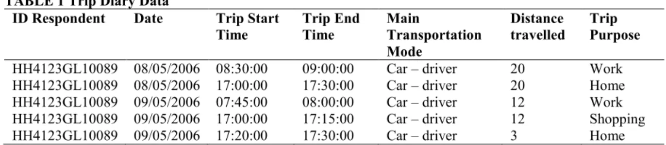
TABLE 1 Trip Diary Data 161
ID Respondent Date Trip Start
Time Trip End Time Main Transportation Mode
Distance
travelled Trip Purpose HH4123GL10089 08/05/2006 08:30:00 09:00:00 Car – driver 20 Work HH4123GL10089 08/05/2006 17:00:00 17:30:00 Car – driver 20 Home HH4123GL10089 09/05/2006 07:45:00 08:00:00 Car – driver 12 Work HH4123GL10089 09/05/2006 17:00:00 17:15:00 Car – driver 12 Shopping HH4123GL10089 09/05/2006 17:20:00 17:30:00 Car – driver 3 Home 162
Table 1 shows a small selection of the trips from the trip diary survey. Only the variables that are relevant for 163
current study are shown here, i.e. the date, the trip start and end time (in Central European Time), the main 164
transportation mode, the distance travelled (in kilometers) and the trip purpose. The GPS data is recorded as 165
GPRMC-strings that contain a time stamp (in Greenwich Mean Time), the latitude and longitude, the speed (in 166
knots), the current direction (measured as an azimuth) and the date. These sentences had already undergone a 167
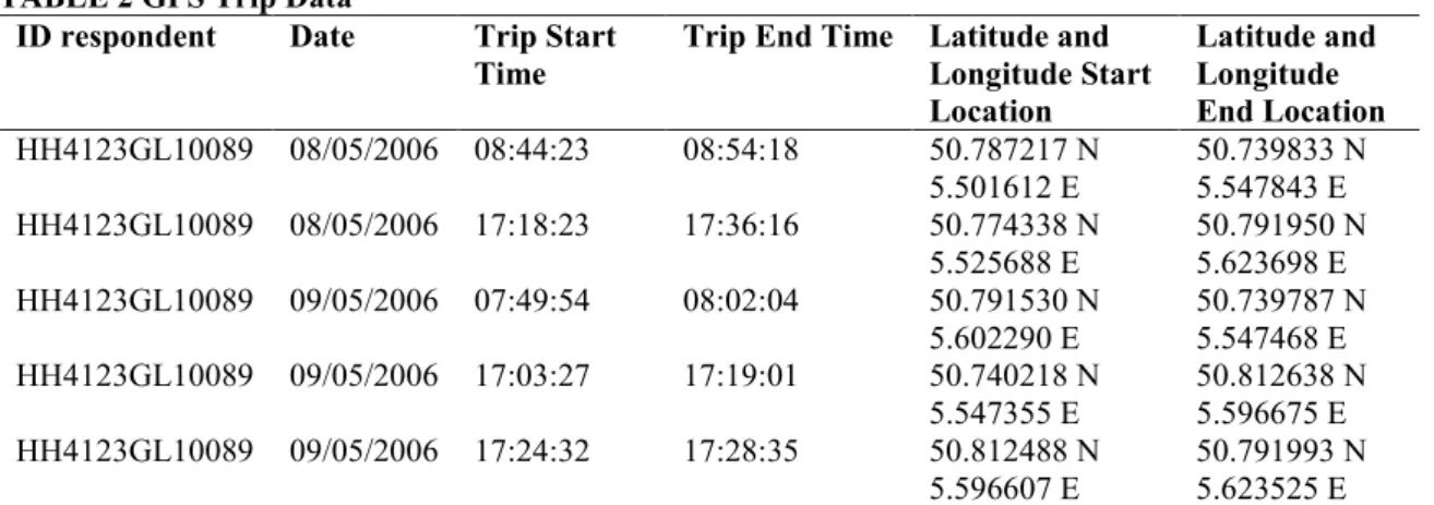
trip end identification procedure as to determine the trips from the raw GPS data. Table 2 shows the information 168
that was obtained from the GPS logs. Here, the trip start and end times are expressed in Central European Time, 169
as to reflect the diary data. Furthermore, the trip start and end times were used to calculate trip durations, both 170
for the diary and the GPS data. 171
172
TABLE 2 GPS Trip Data 173
ID respondent Date Trip Start Time
Trip End Time Latitude and Longitude Start Location Latitude and Longitude End Location HH4123GL10089 08/05/2006 08:44:23 08:54:18 50.787217 N 5.501612 E 50.739833 N 5.547843 E HH4123GL10089 08/05/2006 17:18:23 17:36:16 50.774338 N 5.525688 E 50.791950 N 5.623698 E HH4123GL10089 09/05/2006 07:49:54 08:02:04 50.791530 N 5.602290 E 50.739787 N 5.547468 E HH4123GL10089 09/05/2006 17:03:27 17:19:01 50.740218 N 5.547355 E 50.812638 N 5.596675 E HH4123GL10089 09/05/2006 17:24:32 17:28:35 50.812488 N 5.596607 E 50.791993 N 5.623525 E 174 175 2.2 Data Processing 176 177
The comparison of the two data sources (i.e. the diaries and the GPS logs) shows a certain mismatch in time 178
registration. This mismatch is most likely due to incomplete schedules, the trip end identification process applied 179
during the data processing and cleaning step, but also GPS burn in (i.e. lack of GPS recording due to insufficient 180
satellite signals), battery instability, incorrect diary reporting and incorrect use of GPS devices. For most trips, 181
only a small deviation in time registration was detected, reflecting rounding errors and burn in problems. These 182
deviations could also be depicted when comparing the temporal information in table 1 and the temporal 183
information in table 2. About 5 % of the data, however, show deviations in trip starting times and trip durations 184
that exceed one hour. In case of such discrepancies, the data of that respondents’ day were removed from 185
analysis. It is assumed that these large deviations mainly result from an inaccuracy during the process of trip end 186
identification or during the data cleaning. 187
During the data processing step, both the trip data derived from the activity diaries and the GPS trip 188
data for which matching diary data was available, were converted into activity data sets. The activity before the 189
first and after the last trip of each respondent on each survey day was assumed to be a home activity. 190
Furthermore, the activity start and end times were used to calculate activity durations, both in the diary and in 191
the GPS data. 192
Three variables were considered in the analysis: the activity duration (AD), the activity start time (AST) 193
and the activity type. The activity duration and activity start time are used as explanatory variables to predict the 194
activity type. Both explanatory variables are recorded in Central European Time (CET) and are expressed in 195
minutes, starting from midnight for the activity start time variable (e.g. 660 minutes at 11:00 AM, 900 minutes 196
at 03:00 PM….). CET is 1 hour ahead of Coordinated Universal Time (UTC) (i.e. UTC+01:00). Consequently, 197
the activity start times are specified in CET. The variable activity type has six possible values: home, work, 198
bring/get, leisure (e.g. sports), shopping and social (e.g. visits). 199
The resulting, randomly sampled, training data set consists of 8550 observations (75%), while 2898 200
observations (25%) constitute the validation data set. Both the training and the validation data set concern data 201
that stems from the diary survey. The training set was used to train the model, the validation set to tune the 202
model, e.g. for pruning the decision tree. As indicated by Wets et al. (23), using a random sample of 75 percent 203
of the cases for training and a 25 percent subset for validation is frequently used and judged to be sufficiently 204
reliable. Finally, an independent test set was used to obtain the performance of the model on real-world data. 205
This test set concerns the GPS traces for which corresponding diary data is also available, representing 290 206
activities. 207
3 METHODOLOGY AND RESULTS 208
209
Using the activity data sets, a classification of the activity start times and activity durations was obtained from a 210
decision tree induction. The J48 decision tree-inducing algorithm of the Waikato Environment for Knowledge 211
Analysis (Weka) interface, which is the Weka implementation of C4.5 published by Ross Quinlan in 1993, was 212
applied. Weka is an open-source Java application which consists of a collection of machine learning algorithms 213
for data mining tasks (24). C4.5 was chosen because it is one of the most commonly used algorithms in the 214
machine learning and data mining communities (25). For many domains, the trees produced by C4.5 are both 215
small and accurate, resulting in fast reliable classifiers, and making decision trees a valuable and popular tool for 216
classification (25). In decision trees, each internal node contains a test that decides what branch to follow from 217
that node. C4.5 and its predecessor, ID3, both use formulas based on information theory to evaluate whether a 218
test extracts the maximum amount of information from a set of cases, given the constraint that only one attribute 219
will be tested. The method that is used here for pruning the decision tree estimates the error rate of every subtree 220
and replaces the subtree with a leaf node if the estimated error of the leaf is lower (26). 221
Several decision trees were built on the training set, and evaluated using the validation data set and the 222
test set. The classification was optimized by pruning the tree, i.e. by considering minimum class frequencies and 223
by creating balance between the number of leaf nodes and the degree of impurity. The classification error was 224
used to measure this degree of impurity. By lowering the confidence in the training data not only the tree size 225
was reduced, but statistically irrelevant nodes that would otherwise lead to classification errors were also filtered 226
out. For this, several values for the confidence factor were tested when generating the decision tree to find the 227
most appropriate value for the training set. 228
229
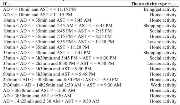
TABLE 3 If-then Rules from Optimal Decision Tree 230
If… Then activity type = …
AD < = 10min and AST < = 11:15 PM Bring/get activity
AD < = 10min and AST > 11:15 PM Home activity
10min < AD < = 35min and AST < = 7:45 AM Home activity 10min < AD < = 35min and 7:45 AM < AST < = 6:45 PM Shopping activity 10min < AD < = 35min and 6:45 PM < AST < = 7:15 PM Social activity 10min < AD < = 35min and 7:15 PM < AST < = 8:55 PM Home activity 10min < AD < = 35min and 8:55 PM < AST < = 11:20 PM Leisure activity 10min < AD < = 35min and AST > 11:20 PM Home activity 35min < AD < = 50min and AST < = 5:45 PM Shopping activity 35min < AD < = 3h30min and 5:45 PM < AST < = 8:30 PM Social activity 35min < AD < = 2h5min and 8:30 PM < AST < = 9:50 PM Leisure activity 35min < AD < = 3h30min and AST > 9:50 PM Home activity 50min < AD < = 3h30min and AST < = 5:45 PM Home activity 2h5min < AD < = 3h30min and 8:30 PM < AST < = 9:50 PM Home activity 3h30min < AD < 14h25min and 2:30 AM < AST < = 9:30 AM Work activity
AD > 3h30min and AST < = 2:30 AM Home activity
AD > 3h30min and AST > 9:30 AM Home activity
AD > 14h25min and 2:30 AM < AST < = 9:30 AM Home activity 231
232
FIGURE 1 Optimal decision tree (DT) for activity type inference. 233
The most optimal classification tree constructed (when considering both in-home and out-of-home activities) 234
comprises 18 leaves, as shown in figure 1. Here, a minimum of 10 activities per leaf and a confidence factor of 235
0.001 were used as pruning conditions. Consequently, 18 if-then rules were derived (see table 3). An accuracy of 236
74% was achieved when training the tree. The accuracy of the model for the validation set, i.e. 72.5%, shows 237
that overfitting is minimal. When applying the model to the (unseen) GPS data, i.e. the test set, the performance 238
was almost 76% accurate. The decision tree classified the activity durations into 7 classes, while the activity start 239
times were categorized into 12 classes. Applying both categorizations to the data set gives a maximum of 84 240
possible categories. However, in several categories no observations are available, and thus for these categories 241
no predictions will be modeled. 242
Some conclusions can be drawn from the if-then rules (table 3) that apply to the most optimal decision 243
tree (figure 1). These results also emerge later on in this paper, in table 5 and table 6. It appears that bring/get 244
activities typically have a short duration and that these activities are performed throughout the entire day. On the 245
other hand, the duration of work activities is much longer. The if-then rules indicate that these activities start 246
mostly in the morning. As expected, the rules that apply to shopping activities are consistent with the opening 247
hours of shopping facilities. Accordingly, activities performed in the (late) evening that last longer than 10 248
minutes are social and leisure activities. 249
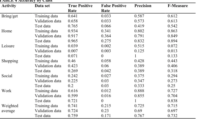
Table 4 shows the true positive rate, false positive rate, precision, and F-measure for each activity type, 250
and for all three data sets. The true positive rate for a specific activity type, e.g. activity x, gives the proportion 251
of examples which were classified as activity x among all examples which truly are activity x. The false positive 252
rate of activity x gives the proportion of examples which were classified as activity x but belong to a different 253
class, among all examples which are not of class x. Furthermore, the precision of class x is the proportion of 254
examples which truly are activity x among all those which were classified as activity x. And finally, the F-255
measure is a combined measure for the precision and true positive rate. 256
257
TABLE 4 Accuracy by Class 258
Activity Data set True Positive Rate
False Positive Rate
Precision F-Measure Bring/get Training data
Validation data Test data 0.641 0.658 0.765 0.033 0.033 0.066 0.587 0.573 0.419 0.612 0.613 0.542
Home Training data
Validation data Test data 0.934 0.917 0.965 0.341 0.364 0.275 0.802 0.791 0.832 0.863 0.849 0.894 Leisure Training data
Validation data Test data 0.039 0.007 0.071 0.002 0.003 0 0.515 0.125 1 0.072 0.013 0.133 Shopping Training data
Validation data Test data 0.46 0.423 0.269 0.058 0.06 0.042 0.428 0.389 0.389 0.443 0.406 0.318 Social Training data
Validation data Test data 0.242 0.225 0.2 0.027 0.03 0.03 0.375 0.347 0.333 0.294 0.273 0.25
Work Training data
Validation data Test data 0.616 0.599 0.721 0.012 0.016 0 0.888 0.855 1 0.727 0.704 0.838 Weighted
average Training data Validation data Test data 0.741 0.724 0.759 0.215 0.23 0.171 0.725 0.69 0.767 0.715 0.697 0.732 259
Table 4 shows that the true positive rate is highest for home activities, in all three data sets, and lowest for 260
leisure activities. When considering the false positive rates, the same conclusions can be drawn. About 80% of 261
the activities that were classified as home activities by the model are truly a home activity. A precision of 1, as is 262
the case for leisure and working activities when applying the model to the test data, indicates that all examples 263
that were classified as leisure and work activities in the test data set were truly leisure and work activities, 264
respectively. However, the low true positive rate of leisure activities indicates that among all the examples that 265
truly are leisure activities, only 7.1% was classified as a leisure activity. The remaining 92.9% of leisure 266
activities in the test data were wrongly classified as a different activity. On the other hand, among all examples 267
which are not leisure activities, there were no examples classified as a leisure activity. The model performed 268
better for work activities, since 72.1% of the work activities in the test set were classified as a work activity, and 269
only 27.9% of work activities were classified as another activity. 270
Based on the decision tree, probability matrices were constructed. For each class of activity start time 271
and activity duration, the probability of conducting the six different activities is predicted. The resulting 272
probabilities, when considering the most optimal classification tree, are shown in table 5. From this probability 273
matrix, a point prediction (majority) matrix was extracted using the highest probabilities per class (see table 6). 274
275
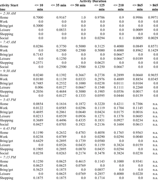
TABLE 5 Probability Matrix 276
Activity Duration Activity Start
Time <= 10 min <= 35 min <= 50 min <= 125 min <= 210 min <= 865 min > 865 min
<= 2:30 AM - Home 0.7000 0.9167 1.0 0.9706 0.9 0.9986 0.9971 - Work 0.0 0.0 0.0 0.0 0.0 0.0 0.0 - Bring/get 0.3000 0.0 0.0 0.0 0.0 0.0 0.0 - Leisure 0.0 0.0833 0.0 0.0 0.0 0.0009 0.0 - Shopping 0.0 0.0 0.0 0.0 0.0 0.0 0.0 - Social 0.0 0.0 0.0 0.0294 0.1 0.0005 0.0029 <= 7:45 AM - Home 0.0286 0.3750 0.5000 0.3125 0.4000 0.0849 0.8571 - Work 0.0 0.2500 0.2500 0.5000 0.4000 0.8962 0.1429 - Bring/get 0.7143 0.0 0.0 0.0 0.0667 0.0 0.0 - Leisure 0.0 0.1250 0.0 0.0 0.0667 0.0189 0.0 - Shopping 0.2571 0.0 0.0 0.0625 0.0 0.0 0.0 - Social 0.0 0.2500 0.2500 0.1250 0.0667 0.0 0.0 <= 9:30 AM - Home 0.0240 0.1392 0.3667 0.2738 0.2899 0.0660 0.9655 - Work 0.0180 0.1139 0.0333 0.2976 0.4889 0.8854 0.0345 - Bring/get 0.7485 0.2532 0.1000 0.0238 0.0111 0.0104 0.0 - Leisure 0.006 0.0127 0.0667 0.1548 0.1111 0.2260 0.0 - Shopping 0.2036 0.4684 0.3000 0.1905 0.0556 0.0017 0.0 - Social 0.0 0.0127 0.1333 0.0595 0.0444 0.0139 0.0 <= 5:45 PM - Home 0.0854 0.1616 0.1872 0.3220 0.4211 0.7306 n.a. - Work 0.0122 0.0585 0.0296 0.1119 0.1704 0.1145 n.a. - Bring/get 0.4695 0.2061 0.0640 0.0424 0.0175 0.0016 n.a. - Leisure 0.0213 0.0539 0.0936 0.1271 0.1378 0.0685 n.a. - Shopping 0.3689 0.4496 0.4335 0.1831 0.0927 0.0234 n.a. - Social 0.0427 0.0703 0.1921 0.2136 0.1604 0.0613 n.a. <= 6:45 PM - Home 0.1190 0.2632 0.4783 0.4058 0.1765 0.9563 n.a. - Work 0.0238 0.0789 0.0 0.0290 0.0294 0.0040 n.a. - Bring/get 0.6429 0.2895 0.1739 0.0580 0.0 0.0 n.a. - Leisure 0.0 0.0526 0.0435 0.1159 0.3824 0.0159 n.a. - Shopping 0.1905 0.2895 0.0870 0.0435 0.0294 0.0 n.a. - Social 0.0238 0.0263 0.2174 0.3478 0.3824 0.0238 n.a. <= 7:15 PM - Home 0.1250 0.0625 0.4615 0.1143 0.1000 0.9341 n.a. - Work 0.0625 0.0625 0.0769 0.0 0.0 0.0 n.a. - Bring/get 0.5625 0.1875 0.0 0.0857 0.0 0.0 n.a. - Leisure 0.0 0.0625 0.0769 0.2857 0.4000 0.0220 n.a. - Shopping 0.1875 0.1875 0.0 0.1714 0.0 0.0 n.a.
- Social 0.0625 0.4375 0.3846 0.3429 0.5000 0.0440 n.a. <= 8:30 PM - Home 0.2174 0.3571 0.3125 0.0741 0.1389 0.9568 n.a. - Work 0.0 0.1429 0.1250 0.0741 0.0278 0.0 n.a. - Bring/get 0.6957 0.2143 0.0625 0.0556 0.0 0.0 n.a. - Leisure 0.0 0.0357 0.0625 0.3519 0.4444 0.0247 n.a. - Shopping 0.0435 0.0714 0.1875 0.0 0.0 0.0 n.a. - Social 0.0435 0.1786 0.2500 0.4444 0.3889 0.0185 n.a. <= 8:55 PM
- Home 0.0 0.5000 0.5000 0.1429 0.8913 n.a. n.a.
- Work 0.2000 0.0 0.0 0.0 0.0 n.a. n.a.
- Bring/get 0.6000 0.5000 0.0 0.0 0.0 n.a. n.a.
- Leisure 0.0 0.0 0.0 0.5714 0.0217 n.a. n.a.
- Shopping 0.2000 0.0 0.5000 0.0 0.0 n.a. n.a.
- Social 0.0 0.0 0.0 0.2857 0.0870 n.a. n.a.
<= 9:50 PM
- Home 0.0 0.0 0.0 0.0 0.9911 n.a. n.a.
- Work 0.0 0.0 0.0 0.0 0.0 n.a. n.a.
- Bring/get 0.8571 0.3333 0.5000 0.1000 0.0 n.a. n.a.
- Leisure 0.0 0.6667 0.5000 0.6000 0.0089 n.a. n.a.
- Shopping 0.1429 0.0 0.0 0.0 0.0 n.a. n.a.
- Social 0.0 0.0 0.0 0.3000 0.0 n.a. n.a.
<= 11:15 PM
- Home 0.0 0.0 1.0 1.0 n.a. n.a. n.a.
- Work 0.0 0.0 0.0 0.0 n.a. n.a. n.a.
- Bring/get 1.0 0.3333 0.0 0.0 n.a. n.a. n.a.
- Leisure 0.0 0.4444 0.0 0.0 n.a. n.a. n.a.
- Shopping 0.0 0.0 0.0 0.0 n.a. n.a. n.a.
- Social 0.0 0.2222 0.0 0.0 n.a. n.a. n.a.
<= 11:20 PM
- Home n.a. n.a. 1.0 n.a. n.a. n.a. n.a.
- Work n.a. n.a. 0.0 n.a. n.a. n.a. n.a.
- Bring/get n.a. n.a. 0.0 n.a. n.a. n.a. n.a.
- Leisure n.a. n.a. 0.0 n.a. n.a. n.a. n.a.
- Shopping n.a. n.a. 0.0 n.a. n.a. n.a. n.a.
- Social n.a. n.a. 0.0 n.a. n.a. n.a. n.a.
> 11:20 PM
- Home 1.0 1.0 n.a. n.a. n.a. n.a. n.a.
- Work 0.0 0.0 n.a. n.a. n.a. n.a. n.a.
- Bring/get 0.0 0.0 n.a. n.a. n.a. n.a. n.a.
- Leisure 0.0 0.0 n.a. n.a. n.a. n.a. n.a.
- Shopping 0.0 0.0 n.a. n.a. n.a. n.a. n.a.
- Social 0.0 0.0 n.a. n.a. n.a. n.a. n.a.
n.a. not available because there is no input data for these classes 277
278
Table 6 should be interpreted as follows: e.g. if an activity is started at 2:30 AM or earlier and that activity has a 279
duration of 10 minutes or less, than there’s a 70% chance that this is a home activity and a 30% chance that it 280
reflects a bring/get activity. 281
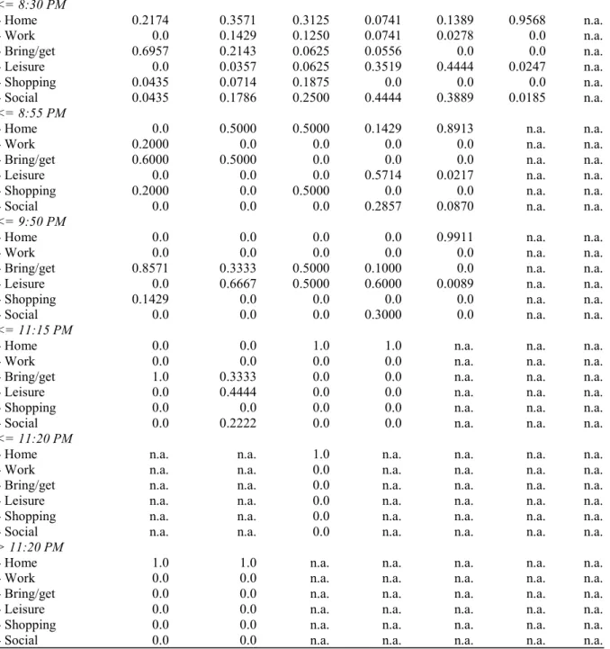
Finally, table 7 shows the majority rules. Here it is clearly shown that activities performed around 282
midnight (i.e. after 11:16 PM but before 2:31 AM) are typically home activities. The same can be said for 283
activity durations of more than 865 minutes. The asterisks in table 7 show for which predictions only weak 284
probabilities were obtained, indicating the significance of the predictions. 285
286 287 288
TABLE 6 Majority Matrix 289
Activity Duration Activity Start
Time <= 10 min <= 35 min <= 50 min <= 125 min <= 210 min <= 865 min > 865 min
<= 2:30 AM Home Home Home Home Home Home Home
<= 7:45 AM Bring/get Home* Home Work Home or
Work*
Work Home
<= 9:30 AM Bring/get Shopping* Home* Work** Work* Work Home
<= 5:45 PM Bring/get* Shopping* Shopping* Home* Home* Home n.a. <= 6:45 PM Bring/get Shopping or
Bring/get**
Home* Home* Leisure or Social*
Home n.a.
<= 7:15 PM Bring/get Social* Home* Social* Social Home n.a.
<= 8:30 PM Bring/get Home* Home* Social* Leisure* Home n.a.
<= 8:55 PM Bring/get Home or Bring/get
Home or Shopping
Leisure Home n.a. n.a.
<= 9:50 PM Bring/get Leisure Bring/get
or Leisure Leisure Home n.a. n.a.
<= 11:15 PM Bring/get Leisure* Home Home n.a. n.a. n.a.
<= 11:20 PM n.a. n.a. Home n.a. n.a. n.a. n.a.
> 11:20 PM Home Home n.a. n.a. n.a. n.a. n.a.
n.a. not available because there is no input data for these classes 290
* weak prediction probability (less than 50%) 291
** weakest prediction probability (i.e. a majority probability of 29,2%) 292
293 294
4 DISCUSSION AND CONCLUSION 295
296
In this paper, a simple and efficient method to annotate (large amounts of) GPS data is presented. The models 297
constructed in this paper indicate the importance of time information in the semantic enrichment process. This 298
paper shows that even when only the temporal dimension of travel diary data is used, reliable and meaningful 299
heuristics can be derived from these diary data. 18 binary if-then rules are presented. Moreover, the high 300
accuracy obtained, by applying the heuristics on independent real-world data (i.e. almost 76%), underlines that 301
the presented heuristics are not data dependent and can be applied to annotate a broad range of GPS data. 302
This study presents a straightforward and readily implemented algorithm. Consequently, the results are 303
relevant for the ongoing development of the next generation of activity-based travel demand models in a cost-304
efficient manner. The contribution of this study towards future data collection is promising in that it enables 305
researchers to directly and automatically infer activities from activity start time and activity duration information 306
obtained from GPS data, without any other additional information. After all, the increasing pervasiveness of 307
location-acquisition technologies, such as GPS, is leading to large collections of spatio-temporal data sets. In 308
addition to the substantial reduction of future data collection efforts for researchers, the results of this study also 309
reduce the associated respondents’ burden of large and demanding diary surveys. Furthermore, the use of the if-310
then rules, combined with technological improvements in the field of GPS devices, can have the potential of 311
increased data accuracy. The results of this research are able to enhance activity-based models, thus resulting in 312
a cost-efficient implementation of sustainable policy measures in traffic and transportation policy and effectively 313
predicting future mobility policy. This research may also contribute in understanding the mental processes 314
individuals go through when making certain traffic related decisions, mainly with respect to activity start times 315
and activity durations. In fact, mobility management requires a thorough knowledge and understanding of 316
individual decision processes. 317
Even though an accuracy of 76% was achieved, this method seems to neglect some of the diversity of 318
the activity type, their time of day and duration. After all, the method depends on identifying typical daily 319
activity patterns based on time of day patterns. The sample is disproportionally made up of the different activity 320
types, therefore possibly inflating the overall accuracy number and masking some inaccurate classifications of 321
social and leisure trips. This implies that the model predicts a more homogeneous set of patterns than a diary-322
based survey would. Hence, more work is needed to address this issue and to achieve the level of accuracy that 323
is required for this approach to become mainstream. 324
Using these models (and further improvements from future research) will enrich GPS logs with diary 325
variables, which enables researches to exclusively use GPS data collection devices. This research contributes to 326
the current scientific state-of-the-art in activity and travel behavior analysis and modeling research, with the goal 327
to apply the results of this study to tens of millions of individual agents. Since the conclusions are solely based 328
on a pure time annotation, future research efforts should extend this concept e.g. by using location information 329
from land use databases, sequential information, or socio-economic data that was obtained in the diary survey, to 330
decide whether a pure time annotation is sufficient to derive meaningful decision rules or to improve the weak 331
predictions from this study. Furthermore, future research efforts should compare these results with the results 332
from several different classifiers and other machine learning techniques. 333
Because of the large deviation in time registration between both data sources, the research methodology 334
should also be applied to other, unrelated data sets, to eliminate additional data biases and overfitting. However, 335
finding more consistent data will be a challenge, since this is a typical travel data problem. 336 337 338 5 REFERENCES 339 340
(1) TRB Committee on Travel Survey Methods. The On-line Travel Survey Manual: A Dynamic Document 341
for Transportation Professionals. Provided by the Members and Friends of the Transportation Research
342
Board’s Travel Survey Methods Committee (ABJ40), Washington, D.C., 2009. 343
http://www.travelsurveymanual.org/. Accessed August 1, 2012. 344
345
(2) Sun, A., S. Sööt, L. Yang, and E. Christopher. Household travel survey nonresponse estimates: The 346
Chicago experience. In Transportation Research Record: Journal of the Transportation Research 347
Record, No. 1493, Transportation Research Board of the National Academies, Washington, D.C., 1995,
348
pp. 170-178. 349
350
(3) Wolf, J. L., R. Guensler, and W. H. Bachman. Elimination of the travel diary: an experiment to derive 351
trip purpose from GPS travel data. In Transportation Research Record: Journal of the Transportation 352
Research Board, No. 1768, Transportation Research Board of the National Academies, Washington,
353
D.C., 2001, pp. 125-134. 354
355
(4) Wolf, J., M. Oliveira, and M. Thompson. Impact of Underreporting on Mileage and Travel Time 356
Estimates: Results from Global Positioning System-Enhanced Household Travel Survey. In 357
Transportation Research Record: Journal of the Transportation Research Board, No. 1854,
358
Transportation Research Board of the National Academies, Washington, D.C., 2003, pp. 189-198. 359
360
(5) Asakura, Y., and E. Hato. Tracking Individual Travel Behaviour using Mobile Phones: Recent 361
Technological Development. In R. Kitamura, T. Yoshii, and T. Yamamoto (eds.). The Expanding 362
Sphere of Travel Behaviour Research: Selected Papers from the 11th International Conference on
363
Travel Behaviour Research. Emerald, Bingley, UK, 2008, pp. 207-223.
364 365
(6) Bullock, P. J., P. R. Stopher, and F. N. F. Horst. Conducting a GPS survey with time-use diary. In 366
Proceedings of the 82nd Annual Meeting of the Transportation Research Board, CD-ROM.
367
Transportation Research Board of the National Academies, Washington, D.C., 2003
368 369
(7) Pendyala, R. M.. Collection and analysis of GPS-based travel data for understanding and modeling 370
activity-travel patterns in time and space. University of South Florida, Tampa, FL, undated. 371
372
(8) Kochan, B., T. Bellemans, D. Janssens, G. Wets, and H. Timmermans. Assessment of the quality of 373
location data obtained by the GPS-enabled PARROTS survey tool. Social Positioning Method 2008, 374
Tartu, Estoni. 375
376
(9) Cools, M., E. Moons, T. Bellemans, D. Janssens, and G. Wets (2009). Surveying activity-travel 377
behavior in Flanders: Assessing the impact of the survey design. In C. Macharis, and L. Turcksin (eds.), 378
Proceedings of the BIVEC-GIBET Transport Research Day 2009, Part II, VUBPress, Brussels, pp.
379
727-741. 380
381
(10) Wolf, J., S. Schönfelder, U. Samaga, M. Oliveira, and K. W. Axhausen. Eighty Weeks of Global 382
Positioning System Traces: Approaches to Enriching Trip Information. In Transportation Research 383
Record: Journal of the Transportation Research Board, No. 1870, Transportation Research Board of
384
the National Academies, Washington, D.C., 2004, pp. 46-54. 385
386
(11) Batelle Transportation Division. Lexington Area Travel Data Collection Test Final Report. Prepared for 387
Federal Highway Administration, Washington, D.C., 1997.
388
(12) Oliveira, M., P. Troped, J. Wolf, C. Matthews, E. Cromley, and S. Melly. Mode and Activity 389
Identification Using GPS and Accelerometer Data. In Proceedings of the 85th Annual Meeting of the
390
Transportation Research Board. CD-ROM. Transportation Research Board of the National Academies,
391
Washington, D.C., 2006. 392
393
(13) Pearson, D. Global Positioning System (GPS) and Travel Surveys: Results from the 1997 Austing 394
Household Survey. Proceedings of the 8th Conference on the Application of Transportation Planning
395
Methods, Texas, 2001.
396 397
(14) Wolf, J. Using GPS Data Loggers to Replace Travel Diaries in the Collection of Travel Data. Thesis, 398
Georgia Institute of Technology, Atlanta, 2000. 399
400
(15) Deng, Z., and M. Ji. Deriving Rules for Trip Purpose Identification from GPS Travel Survey Data and 401
Land Use Data: A Machine Learning Approach. Traffic and Transportation Studies 2010, pp. 768-777. 402
403
(16) Stopher, P., E. Clifford, J. Zhang, and C. FitzGerald. Deducing Mode and Purpose from GPS Data. 404
Proceedings of the Transportation Planning Applications Conference of the Transportation Research
405
Board, Florida, 2007.
406 407
(17) McGowen, P. Predicting Activity Types from GPS and GIS data. Dissertation, University of California, 408
Irvine, 2006. 409
410
(18) Schuessler, N., and K. W. Axhausen. Identifying trips and activities and their characteristics from GPS 411
raw data only. Proceedings of the 8th International Conference on Survey Methods in Transport,
412
Annecy, 2009. 413
414
(19) Schuessler, N., and K. W. Axhausen. Processing Raw Data from Globel Positioning Systems Without 415
Additional Information. In Transportation Research Record: Journal of the Transportation Research 416
Board, No. 2105, Transportation Research Board of the National Academies, Washington, D.C., 2009,
417
pp. 28-36. 418
419
(20) Zheng, Y., Y. Chen, Q. Li, X. Xie, and W.-Y. Ma. Understanding Transportation Modes Based on GPS 420
Data for Web Applications. ACM Transactions on the Web, Vol. 4, No. 1, 2010, pp. 1-36. 421
422
(21) Drazin, S., and M. Montag. Decision Tree Analysis using Weka Machine Learning Project II. 423
University of Miami, undated, pp. 1-3. 424
425
(22) Bellemans, T., B. Kochan, D. Janssens, G. Wets, and H. Timmermans. Field Evaluation of Personal 426
Digital Assistant Enabled by Global Positioning System: Impact on Quality of Activity and Diary Data. 427
In Transportation Research Record: Journal of the Transportation Research Board, No. 2049, 428
Transportation Research Board of the National Academies, Washington, D.C., 2008, pp. 136-143. 429
430
(23) Wets, G., K. Vanhoof, T. Arentze, and H. Timmermans. Identifying Decision Structures Underlying 431
Activity Patterns: Exploration of Data Mining Algorithms. In Transportation Research Record: 432
Journal of the Transportation Research Board, No. 1718, Transportation Research Board of the
433
National Academies, Washington, D.C., 2000, pp. 1-9. 434
435
(24) Witten, I. H., E. Frank, and M. A. Hall. Data Mining: Practical Machine Learning Tools and 436
Techniques. Elsevier Inc., Burlington, 2011.
437 438
(25) Drummond, C., and R. C. Holte, R. C. C4.5, Class Imbalance, and Cost Sensitivity: Why Under-439
Sampling beats Over-Sampling. Workshop on Learning from Imbalanced Datasets II, Washington, 440
D.C., 2003. 441
442
(26) Salzberg, S. L. Book Review: C4.5: Programs for Machine Learning by J. Ross Quinlan. Morgan 443
Kaufmann Publishers, Inc. 1993. Machine Learning, Vol. 16, No. 3, 1994, pp. 235-240. 444